
Содержание
- Use Excel built-in functions to find data in a table or a range of cells
- Summary
- Create the Sample Worksheet
- Term Definitions
- Functions
- LOOKUP()
- VLOOKUP()
- INDEX() and MATCH()
- OFFSET() and MATCH()
- Find and select cells that meet specific conditions
- Need more help?
- Find and select cells that meet specific conditions
- Need more help?
- Поиск данных в таблице или диапазоне ячеек с помощью встроенных функций Excel
- Описание
- Создание образца листа
- Определения терминов
- Функции
- LOOKUP ()
- INDEX () и MATCH ()
- СМЕЩ () и MATCH ()
Use Excel built-in functions to find data in a table or a range of cells
Summary
This step-by-step article describes how to find data in a table (or range of cells) by using various built-in functions in Microsoft Excel. You can use different formulas to get the same result.
Create the Sample Worksheet
This article uses a sample worksheet to illustrate Excel built-in functions. Consider the example of referencing a name from column A and returning the age of that person from column C. To create this worksheet, enter the following data into a blank Excel worksheet.
You will type the value that you want to find into cell E2. You can type the formula in any blank cell in the same worksheet.
Term Definitions
This article uses the following terms to describe the Excel built-in functions:
The whole lookup table
The value to be found in the first column of Table_Array.
Lookup_Array
-or-
Lookup_Vector
The range of cells that contains possible lookup values.
The column number in Table_Array the matching value should be returned for.
3 (third column in Table_Array)
Result_Array
-or-
Result_Vector
A range that contains only one row or column. It must be the same size as Lookup_Array or Lookup_Vector.
A logical value (TRUE or FALSE). If TRUE or omitted, an approximate match is returned. If FALSE, it will look for an exact match.
This is the reference from which you want to base the offset. Top_Cell must refer to a cell or range of adjacent cells. Otherwise, OFFSET returns the #VALUE! error value.
This is the number of columns, to the left or right, that you want the upper-left cell of the result to refer to. For example, «5» as the Offset_Col argument specifies that the upper-left cell in the reference is five columns to the right of reference. Offset_Col can be positive (which means to the right of the starting reference) or negative (which means to the left of the starting reference).
Functions
LOOKUP()
The LOOKUP function finds a value in a single row or column and matches it with a value in the same position in a different row or column.
The following is an example of LOOKUP formula syntax:
The following formula finds Mary’s age in the sample worksheet:
The formula uses the value «Mary» in cell E2 and finds «Mary» in the lookup vector (column A). The formula then matches the value in the same row in the result vector (column C). Because «Mary» is in row 4, LOOKUP returns the value from row 4 in column C (22).
NOTE: The LOOKUP function requires that the table be sorted.
For more information about the LOOKUP function, click the following article number to view the article in the Microsoft Knowledge Base:
VLOOKUP()
The VLOOKUP or Vertical Lookup function is used when data is listed in columns. This function searches for a value in the left-most column and matches it with data in a specified column in the same row. You can use VLOOKUP to find data in a sorted or unsorted table. The following example uses a table with unsorted data.
The following is an example of VLOOKUP formula syntax:
The following formula finds Mary’s age in the sample worksheet:
The formula uses the value «Mary» in cell E2 and finds «Mary» in the left-most column (column A). The formula then matches the value in the same row in Column_Index. This example uses «3» as the Column_Index (column C). Because «Mary» is in row 4, VLOOKUP returns the value from row 4 in column C (22).
For more information about the VLOOKUP function, click the following article number to view the article in the Microsoft Knowledge Base:
INDEX() and MATCH()
You can use the INDEX and MATCH functions together to get the same results as using LOOKUP or VLOOKUP.
The following is an example of the syntax that combines INDEX and MATCH to produce the same results as LOOKUP and VLOOKUP in the previous examples:
The following formula finds Mary’s age in the sample worksheet:
The formula uses the value «Mary» in cell E2 and finds «Mary» in column A. It then matches the value in the same row in column C. Because «Mary» is in row 4, the formula returns the value from row 4 in column C (22).
NOTE: If none of the cells in Lookup_Array match Lookup_Value («Mary»), this formula will return #N/A.
For more information about the INDEX function, click the following article number to view the article in the Microsoft Knowledge Base:
OFFSET() and MATCH()
You can use the OFFSET and MATCH functions together to produce the same results as the functions in the previous example.
The following is an example of syntax that combines OFFSET and MATCH to produce the same results as LOOKUP and VLOOKUP:
This formula finds Mary’s age in the sample worksheet:
The formula uses the value «Mary» in cell E2 and finds «Mary» in column A. The formula then matches the value in the same row but two columns to the right (column C). Because «Mary» is in column A, the formula returns the value in row 4 in column C (22).
For more information about the OFFSET function, click the following article number to view the article in the Microsoft Knowledge Base:
Источник
Find and select cells that meet specific conditions
Use the Go To command to quickly find and select all cells that contain specific types of data, such as formulas. Also, use Go To to find only the cells that meet specific criteria,—such as the last cell on the worksheet that contains data or formatting.
Follow these steps:
Begin by doing either of the following:
To search the entire worksheet for specific cells, click any cell.
To search for specific cells within a defined area, select the range, rows, or columns that you want. For more information, see Select cells, ranges, rows, or columns on a worksheet.
Tip: To cancel a selection of cells, click any cell on the worksheet.
On the Home tab, click Find & Select > Go To (in the Editing group).
Keyboard shortcut: Press CTRL+G.
In the Go To Special dialog box, click one of the following options.
Cells that contain comments.
Cells that contain constants.
Cells that contain formulas.
Note: The check boxes below Formulas define the type of formula.
The current region, such as an entire list.
An entire array if the active cell is contained in an array.
Graphical objects, including charts and buttons, on the worksheet and in text boxes.
All cells that differ from the active cell in a selected row. There is always one active cell in a selection—whether this is a range, row, or column. By pressing the Enter or Tab key, you can change the location of the active cell, which by default is the first cell in a row.
If more than one row is selected, the comparison is done for each individual row of that selection, and the cell that is used in the comparison for each additional row is located in the same column as the active cell.
All cells that differ from the active cell in a selected column. There is always one active cell in a selection, whether this is a range, row, or column. By pressing the Enter or Tab key, you can change the location of the active cell—which by default is the first cell in a column.
When selecting more than one column, the comparison is done for each individual column of that selection. The cell that is used in the comparison for each additional column is located in the same row as the active cell.
Cells that are referenced by the formula in the active cell. Under Dependents, do either of the following:
Click Direct only to find only cells that are directly referenced by formulas.
Click All levels to find all cells that are directly or indirectly referenced by the cells in the selection.
Cells with formulas that refer to the active cell. Do either of the following:
Click Direct only to find only cells with formulas that refer directly to the active cell.
Click All levels to find all cells that directly or indirectly refer to the active cell.
The last cell on the worksheet that contains data or formatting.
Visible cells only
Only cells that are visible in a range that crosses hidden rows or columns.
Only cells that have conditional formats applied. Under Data validation, do either of the following:
Click All to find all cells that have conditional formats applied.
Click Same to find cells that have the same conditional formats as the currently selected cell.
Only cells that have data validation rules applied. Do either of the following:
Click All to find all cells that have data validation applied.
Click Same to find cells that have the same data validation as the currently selected cell.
Need more help?
You can always ask an expert in the Excel Tech Community or get support in the Answers community.
Источник
Поиск данных в таблице или диапазоне ячеек с помощью встроенных функций Excel
Примечание: Мы стараемся как можно оперативнее обеспечивать вас актуальными справочными материалами на вашем языке. Эта страница переведена автоматически, поэтому ее текст может содержать неточности и грамматические ошибки. Для нас важно, чтобы эта статья была вам полезна. Просим вас уделить пару секунд и сообщить, помогла ли она вам, с помощью кнопок внизу страницы. Для удобства также приводим ссылку на оригинал (на английском языке).
Описание
В этой статье приведены пошаговые инструкции по поиску данных в таблице (или диапазоне ячеек) с помощью различных встроенных функций Microsoft Excel. Для получения одного и того же результата можно использовать разные формулы.
Создание образца листа
В этой статье используется образец листа для иллюстрации встроенных функций Excel. Рассматривайте пример ссылки на имя из столбца A и возвращает возраст этого человека из столбца C. Чтобы создать этот лист, введите указанные ниже данные в пустой лист Excel.
Введите значение, которое вы хотите найти, в ячейку E2. Вы можете ввести формулу в любую пустую ячейку на том же листе.
Определения терминов
В этой статье для описания встроенных функций Excel используются указанные ниже условия.
Вся таблица подстановки
Значение, которое будет найдено в первом столбце аргумента «инфо_таблица».
Просматриваемый_массив
-или-
Лукуп_вектор
Диапазон ячеек, которые содержат возможные значения подстановки.
Номер столбца в аргументе инфо_таблица, для которого должно быть возвращено совпадающее значение.
3 (третий столбец в инфо_таблица)
Ресулт_аррай
-или-
Ресулт_вектор
Диапазон, содержащий только одну строку или один столбец. Он должен быть такого же размера, что и просматриваемый_массив или Лукуп_вектор.
Логическое значение (истина или ложь). Если указано значение истина или опущено, возвращается приближенное соответствие. Если задано значение FALSE, оно будет искать точное совпадение.
Это ссылка, на основе которой вы хотите основать смещение. Топ_целл должен ссылаться на ячейку или диапазон смежных ячеек. В противном случае функция СМЕЩ возвращает #VALUE! значение ошибки #ИМЯ?.
Число столбцов, находящегося слева или справа от которых должна указываться верхняя левая ячейка результата. Например, значение «5» в качестве аргумента Оффсет_кол указывает на то, что верхняя левая ячейка ссылки состоит из пяти столбцов справа от ссылки. Оффсет_кол может быть положительным (то есть справа от начальной ссылки) или отрицательным (то есть слева от начальной ссылки).
Функции
LOOKUP ()
Функция Просмотр находит значение в одной строке или столбце и сопоставляет его со значением в той же позицией в другой строке или столбце.
Ниже приведен пример синтаксиса формулы подСТАНОВКи.
= Просмотр (искомое_значение; Лукуп_вектор; Ресулт_вектор)
Следующая формула находит возраст Марии на листе «образец».
= ПРОСМОТР (E2; A2: A5; C2: C5)
Формула использует значение «Мария» в ячейке E2 и находит слово «Мария» в векторе подстановки (столбец A). Формула затем соответствует значению в той же строке в векторе результатов (столбец C). Так как «Мария» находится в строке 4, функция Просмотр возвращает значение из строки 4 в столбце C (22).
Примечание. Для функции Просмотр необходимо, чтобы таблица была отсортирована.
Чтобы получить дополнительные сведения о функции Просмотр , щелкните следующий номер статьи базы знаний Майкрософт:
Функция ВПР или вертикальный просмотр используется, если данные указаны в столбцах. Эта функция выполняет поиск значения в левом столбце и сопоставляет его с данными в указанном столбце в той же строке. Функцию ВПР можно использовать для поиска данных в отсортированных или несортированных таблицах. В следующем примере используется таблица с несортированными данными.
Ниже приведен пример синтаксиса формулы ВПР :
= ВПР (искомое_значение; инфо_таблица; номер_столбца; интервальный_просмотр)
Следующая формула находит возраст Марии на листе «образец».
= ВПР (E2; A2: C5; 3; ЛОЖЬ)
Формула использует значение «Мария» в ячейке E2 и находит слово «Мария» в левом столбце (столбец A). Формула затем совпадет со значением в той же строке в Колумн_индекс. В этом примере используется «3» в качестве Колумн_индекс (столбец C). Так как «Мария» находится в строке 4, функция ВПР возвращает значение из строки 4 В столбце C (22).
Чтобы получить дополнительные сведения о функции ВПР , щелкните следующий номер статьи базы знаний Майкрософт:
INDEX () и MATCH ()
Вы можете использовать функции индекс и ПОИСКПОЗ вместе, чтобы получить те же результаты, что и при использовании поиска или функции ВПР.
Ниже приведен пример синтаксиса, объединяющего индекс и Match для получения одинаковых результатов поиска и ВПР в предыдущих примерах:
= Индекс (инфо_таблица; MATCH (искомое_значение; просматриваемый_массив; 0); номер_столбца)
Следующая формула находит возраст Марии на листе «образец».
= ИНДЕКС (A2: C5; MATCH (E2; A2: A5; 0); 3)
Формула использует значение «Мария» в ячейке E2 и находит слово «Мария» в столбце A. Затем он будет соответствовать значению в той же строке в столбце C. Так как «Мария» находится в строке 4, формула возвращает значение из строки 4 в столбце C (22).
Обратите внимание Если ни одна из ячеек в аргументе «число» не соответствует искомому значению («Мария»), эта формула будет возвращать #N/А.
Чтобы получить дополнительные сведения о функции индекс , щелкните следующий номер статьи базы знаний Майкрософт:
СМЕЩ () и MATCH ()
Функции СМЕЩ и ПОИСКПОЗ можно использовать вместе, чтобы получить те же результаты, что и функции в предыдущем примере.
Ниже приведен пример синтаксиса, объединяющего смещение и сопоставление для достижения того же результата, что и функция Просмотр и ВПР.
= СМЕЩЕНИЕ (топ_целл, MATCH (искомое_значение; просматриваемый_массив; 0); Оффсет_кол)
Эта формула находит возраст Марии на листе «образец».
= СМЕЩЕНИЕ (A1; MATCH (E2; A2: A5; 0); 2)
Формула использует значение «Мария» в ячейке E2 и находит слово «Мария» в столбце A. Формула затем соответствует значению в той же строке, но двум столбцам справа (столбец C). Так как «Мария» находится в столбце A, формула возвращает значение в строке 4 в столбце C (22).
Чтобы получить дополнительные сведения о функции СМЕЩ , щелкните следующий номер статьи базы знаний Майкрософт:
Источник
You can quickly locate and select specific cells or ranges by entering their names or cell references in the Name box, which is located to the left of the formula bar:

You can also select named or unnamed cells or ranges by using the Go To (F5 or Ctrl+G) command.
Important: To select named cells and ranges, you need to define them first. See Define and use names in formulas for more information.
-
To select a named cell or range, click the arrow next to the Name box to display the list of named cells or ranges, and then click the name that you want.
-
To select two or more named cell references or ranges, click the arrow next to the Name box, and then click the name of the first cell reference or range that you want to select. Then, hold down CTRL while you click the names of other cells or ranges in the Name box.
-
To select an unnamed cell reference or range, type the cell reference of the cell or range of cells that you want to select, and then press ENTER. For example, type B3 to select that cell, or type B1:B3 to select a range of cells.
Note: You can’t delete or change names that have been defined for cells or ranges in the Name box. You can only delete or change names in the Name Manager (Formulas tab, Defined Names group). For more information, see Define and use names in formulas.
-
Press F5 or CTRL+G to launch the Go To dialog.
-
In the Go to list, click the name of the cell or range that you want to select, or type the cell reference in the Reference box, then press OK.
For example, in the Reference box, type B3 to select that cell, or type B1:B3 to select a range of cells. You can select multiple cells or ranges by entering them in the Reference box separated by commas. If you’re referring to a spilled range created by a dynamic array formula, then you can add the spilled range operator. For example, if you have an array in cells A1:A4, you can select it by entering A1# in the Reference box, then press OK.
Tip: To quickly find and select all cells that contain specific types of data (such as formulas) or only cells that meet specific criteria (such as visible cells only or the last cell on the worksheet that contains data or formatting), click Special in the Go To popup window, and then click the option that you want.
-
Go to Formulas > Defined Names > Name Manager.
-
Select the name you want to edit or delete.
-
Choose Edit or Delete.
Hold down the Ctrl key, and left-click each cell or range you want to include. If you over select, you can click on the unintended cell to de-select it.
When you select data for Bing Maps, make sure it is location data — city names, country names, etc. Otherwise, Bing has nothing to map.
To select the cells, you can type a reference in the Select Data dialog box, or click the collapse arrow in the dialog box and select the cells by clicking them. See the preceding sections for more options for selecting the cells you want.
When you select data for Euro Conversion, make sure it is currency data.
To select the cells, you can type a reference in the Source Data box, or click the collapse arrow beside the box and then select the cells by clicking them. See the preceding sections for more options for selecting the cells you want.
You can select adjacent cells in Excel for the web by clicking a cell and dragging to extend the range. However, you can’t select specific cells or a range if they’re not next to each other. If you have the Excel desktop application, you can open your workbook in Excel and select non-adjacent cells by clicking them while holding down the Ctrl key. For more information, see Select specific cells or ranges in Excel.
When using lookup formulas in Excel (such as VLOOKUP, XLOOKUP, or INDEX/MATCH), the intent is to find the matching value and get that value (or a corresponding value in the same row/column) as the result.
But in some cases, instead of getting the value, you may want the formula to return the cell address of the value.
This could be especially useful if you have a large data set and you want to find out the exact position of the lookup formula result.
There are some functions in Excel that designed to do exactly this.
In this tutorial, I will show you how you can find and return the cell address instead of the value in Excel using simple formulas.
Lookup And Return Cell Address Using the ADDRESS Function
The ADDRESS function in Excel is meant to exactly this.
It takes the row and the column number and gives you the cell address of that specific cell.
Below is the syntax of the ADDRESS function:
=ADDRESS(row_num, column_num, [abs_num], [a1], [sheet_text])
where:
- row_num: Row number of the cell for which you want the cell address
- column_num: Column number of the cell for which you want the address
- [abs_num]: Optional argument where you can specify whether want the cell reference to be absolute, relative, or mixed.
- [a1]: Optional argument where you can specify whether you want the reference in the R1C1 style or A1 style
- [sheet_text]: Optional argument where you can specify whether you want to add the sheet name along with the cell address or not
Now, let’s take an example and see how this works.
Suppose there is a dataset as shown below, where I have the Employee id, their name, and their department, and I want to quickly know the cell address that contains the department for employee id KR256.
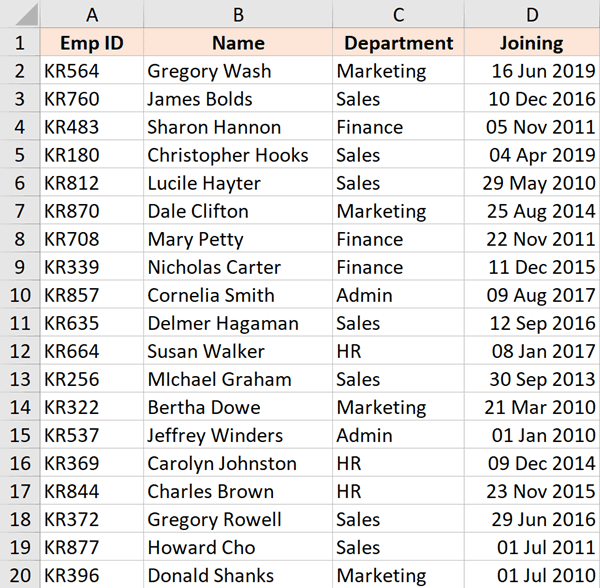
Below is the formula that will do this:
=ADDRESS(MATCH("KR256",A1:A20,0),3)
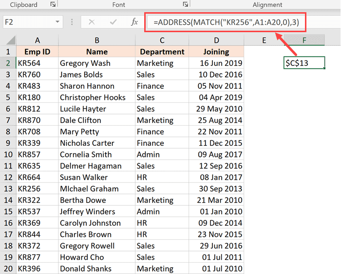
In the above formula, I have used the MATCH function to find out the row number that contains the given employee id.
And since the department is in column C, I have used 3 as the second argument.
This formula works great, but it has one drawback – it won’t work if you add the row above the dataset or a column to the left of the dataset.
This is because when I specify the second argument (the column number) as 3, it’s hard-coded and won’t change.
In case I add any column to the left of the dataset, the formula would count 3 columns from the beginning of the worksheet and not from the beginning of the dataset.
So, if you have a fixed dataset and need a simple formula, this will work fine.
But if you need this to be more fool-proof, use the one covered in the next section.
Lookup And Return Cell Address Using the CELL Function
While the ADDRESS function was made specifically to give you the cell reference of the specified row and column number, there is another function that also does this.
It’s called the CELL function (and it can give you a lot more information about the cell than the ADDRESS function).
Below is the syntax of the CELL function:
=CELL(info_type, [reference])
where:
- info_type: the information about the cell you want. This could be the address, the column number, the file name, etc.
- [reference]: Optional argument where you can specify the cell reference for which you need the cell information.
Now, let’s see an example where you can use this function to look up and get the cell reference.
Suppose you have a dataset as shown below, and you want to quickly know the cell address that contains the department for employee id KR256.
Below is the formula that will do this:
=CELL("address", INDEX($A$1:$D$20,MATCH("KR256",$A$1:$A$20,0),3))
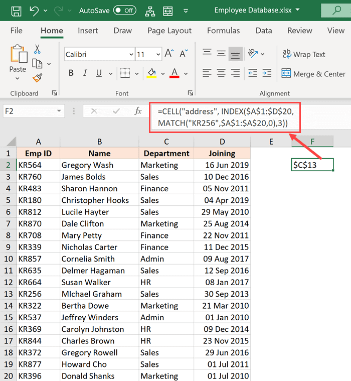
The above formula is quite straightforward.
I have used the INDEX formula as the second argument to get the department for the employee id KR256.
And then simply wrapped it within the CELL function and asked it to return the cell address of this value that I get from the INDEX formula.
Now here is the secret to why it works – the INDEX formula returns the lookup value when you give it all the necessary arguments. But at the same time, it would also return the cell reference of that resulting cell.
In our example, the INDEX formula returns “Sales” as the resulting value, but at the same time, you can also use it to give you the cell reference of that value instead of the value itself.
Normally, when you enter the INDEX formula in a cell, it returns the value because that is what it’s expected to do. But in scenarios where a cell reference is required, the INDEX formula will give you the cell reference.
In this example, that’s exactly what it does.
And the best part about using this formula is that it is not tied to the first cell in the worksheet. This means that you can select any data set (which could be anywhere in the worksheet), use the INDEX formula to do a regular look up and it would still give you the correct address.
And if you insert an additional row or column, the formula would adjust accordingly to give you the correct cell address.
So these are two simple formulas that you can use to look up and find and return the cell address instead of the value in Excel.
I hope you found this tutorial useful.
Other Excel tutorials you may also like:
- Lookup and Return Values in an Entire Row/Column in Excel
- Find the Last Occurrence of a Lookup Value a List in Excel
- Lookup the Second, the Third, or the Nth Value in Excel
- How to Reference Another Sheet or Workbook in Excel
- Lookup and Return Values in an Entire Row/Column in Excel

Поиск какого-либо значения в ячейках Excel довольно часто встречающаяся задача при программировании какого-либо макроса. Решить ее можно разными способами. Однако, в разных ситуациях использование того или иного способа может быть не оправданным. В данной статье я рассмотрю 2 наиболее распространенных способа.
Поиск перебором значений
Довольно простой в реализации способ. Например, найти в колонке «A» ячейку, содержащую «123» можно примерно так:
Sheets("Данные").Select
For y = 1 To Cells.SpecialCells(xlLastCell).Row
    If Cells(y, 1) = "123" Then
        Exit For
    End If
Next y
MsgBox "Нашел в строке: " + CStr(y)
Минусами этого так сказать «классического» способа являются: медленная работа и громоздкость. А плюсом является его гибкость, т.к. таким способом можно реализовать сколь угодно сложные варианты поиска с различными вычислениями и т.п.
Поиск функцией Find
Гораздо быстрее обычного перебора и при этом довольно гибкий. В простейшем случае, чтобы найти в колонке A ячейку, содержащую «123» достаточно такого кода:
Sheets("Данные").Select
Set fcell = Columns("A:A").Find("123")
If Not fcell Is Nothing Then
    MsgBox "Нашел в строке: " + CStr(fcell.Row)
End If
Вкратце опишу что делают строчки данного кода:
1-я строка: Выбираем в книге лист «Данные»;
2-я строка: Осуществляем поиск значения «123» в колонке «A», результат поиска будет в fcell;
3-я строка: Если удалось найти значение, то fcell будет содержать Range-объект, в противном случае — будет пустой, т.е. Nothing.
Полностью синтаксис оператора поиска выглядит так:
Find(What, After, LookIn, LookAt, SearchOrder, SearchDirection, MatchCase, MatchByte, SearchFormat)
What — Строка с текстом, который ищем или любой другой тип данных Excel
After — Ячейка, после которой начать поиск. Обратите внимание, что это должна быть именно единичная ячейка, а не диапазон. Поиск начинается после этой ячейки, а не с нее. Поиск в этой ячейке произойдет только когда весь диапазон будет просмотрен и поиск начнется с начала диапазона и до этой ячейки включительно.
LookIn — Тип искомых данных. Может принимать одно из значений: xlFormulas (формулы), xlValues (значения), или xlNotes (примечания).
LookAt — Одно из значений: xlWhole (полное совпадение) или xlPart (частичное совпадение).
SearchOrder — Одно из значений: xlByRows (просматривать по строкам) или xlByColumns (просматривать по столбцам)
SearchDirection — Одно из значений: xlNext (поиск вперед) или xlPrevious (поиск назад)
MatchCase — Одно из значений: True (поиск чувствительный к регистру) или False (поиск без учета регистра)
MatchByte — Применяется при использовании мультибайтных кодировок: True (найденный мультибайтный символ должен соответствовать только мультибайтному символу) или False (найденный мультибайтный символ может соответствовать однобайтному символу)
SearchFormat — Используется вместе с FindFormat. Сначала задается значение FindFormat (например, для поиска ячеек с курсивным шрифтом так: Application.FindFormat.Font.Italic = True), а потом при использовании метода Find указываем параметр SearchFormat = True. Если при поиске не нужно учитывать формат ячеек, то нужно указать SearchFormat = False.
Чтобы продолжить поиск, можно использовать FindNext (искать «далее») или FindPrevious (искать «назад»).
Примеры поиска функцией Find
Пример 1: Найти в диапазоне «A1:A50» все ячейки с текстом «asd» и поменять их все на «qwe»
With Worksheets(1).Range("A1:A50")
  Set c = .Find("asd", LookIn:=xlValues)
  Do While Not c Is Nothing
    c.Value = "qwe"
    Set c = .FindNext(c)
  Loop
End With
Обратите внимание: Когда поиск достигнет конца диапазона, функция продолжит искать с начала диапазона. Таким образом, если значение найденной ячейки не менять, то приведенный выше пример зациклится в бесконечном цикле. Поэтому, чтобы этого избежать (зацикливания), можно сделать следующим образом:
Пример 2: Правильный поиск значения с использованием FindNext, не приводящий к зацикливанию.
With Worksheets(1).Range("A1:A50")
  Set c = .Find("asd", lookin:=xlValues)
  If Not c Is Nothing Then
    firstResult = c.Address
    Do
      c.Font.Bold = True
      Set c = .FindNext(c)
      If c Is Nothing Then Exit Do
    Loop While c.Address <> firstResult
  End If
End With
В ниже следующем примере используется другой вариант продолжения поиска — с помощью той же функции Find с параметром After. Когда найдена очередная ячейка, следующий поиск будет осуществляться уже после нее. Однако, как и с FindNext, когда будет достигнут конец диапазона, Find продолжит поиск с его начала, поэтому, чтобы не произошло зацикливания, необходимо проверять совпадение с первым результатом поиска.
Пример 3: Продолжение поиска с использованием Find с параметром After.
With Worksheets(1).Range("A1:A50")
  Set c = .Find("asd", lookin:=xlValues)
  If Not c Is Nothing Then
    firstResult = c.Address
    Do
      c.Font.Bold = True
      Set c = .Find("asd", After:=c, lookin:=xlValues)
      If c Is Nothing Then Exit Do
    Loop While c.Address <> firstResult
  End If
End With
Следующий пример демонстрирует применение SearchFormat для поиска по формату ячейки. Для указания формата необходимо задать свойство FindFormat.
Пример 4: Найти все ячейки с шрифтом «курсив» и поменять их формат на обычный (не «курсив»)
lLastRow = Cells.SpecialCells(xlLastCell).Row
lLastCol = Cells.SpecialCells(xlLastCell).Column
Application.FindFormat.Font.Italic = True
With Worksheets(1).Range(Cells(1, 1), Cells(lLastRow, lLastCol))
  Set c = .Find("", SearchFormat:=True)
  Do While Not c Is Nothing
    c.Font.Italic = False
    Set c = .Find("", After:=c, SearchFormat:=True)
  Loop
End With
Примечание: В данном примере намеренно не используется FindNext для поиска следующей ячейки, т.к. он не учитывает формат (статья об этом: https://support.microsoft.com/ru-ru/kb/282151)
Коротко опишу алгоритм поиска Примера 4. Первые две строки определяют последнюю строку (lLastRow) на листе и последний столбец (lLastCol). 3-я строка задает формат поиска, в данном случае, будем искать ячейки с шрифтом Italic. 4-я строка определяет область ячеек с которой будет работать программа (с ячейки A1 и до последней строки и последнего столбца). 5-я строка осуществляет поиск с использованием SearchFormat. 6-я строка — цикл пока результат поиска не будет пустым. 7-я строка — меняем шрифт на обычный (не курсив), 8-я строка продолжаем поиск после найденной ячейки.
Хочу обратить внимание на то, что в этом примере я не стал использовать «защиту от зацикливания», как в Примерах 2 и 3, т.к. шрифт меняется и после «прохождения» по всем ячейкам, больше не останется ни одной ячейки с курсивом.
Свойство FindFormat можно задавать разными способами, например, так:
With Application.FindFormat.Font
  .Name = "Arial"
  .FontStyle = "Regular"
  .Size = 10
End With
Поиск последней заполненной ячейки с помощью Find
Следующий пример — применение функции Find для поиска последней ячейки с заполненными данными. Использованные в Примере 4 SpecialCells находит последнюю ячейку даже если она не содержит ничего, но отформатирована или в ней раньше были данные, но были удалены.
Пример 5: Найти последнюю колонку и столбец, заполненные данными
Set c = Worksheets(1).UsedRange.Find("*", SearchDirection:=xlPrevious)
If Not c Is Nothing Then
  lLastRow = c.Row: lLastCol = c.Column
Else
  lLastRow = 1: lLastCol = 1
End If
MsgBox "lLastRow=" & lLastRow & " lLastCol=" & lLastCol
В этом примере используется UsedRange, который так же как и SpecialCells возвращает все используемые ячейки, в т.ч. и те, что были использованы ранее, а сейчас пустые. Функция Find ищет ячейку с любым значением с конца диапазона.
Поиск по шаблону (маске)
При поиске можно так же использовать шаблоны, чтобы найти текст по маске, следующий пример это демонстрирует.
Пример 6: Выделить красным шрифтом ячейки, в которых текст начинается со слова из 4-х букв, первая и последняя буквы «т», при этом после этого слова может следовать любой текст.
With Worksheets(1).Cells
  Set c = .Find("т??т*", LookIn:=xlValues, LookAt:=xlWhole)
  If Not c Is Nothing Then
    firstResult = c.Address
    Do
      c.Font.Color = RGB(255, 0, 0)
      Set c = .FindNext(c)
      If c Is Nothing Then Exit Do
    Loop While c.Address <> firstResult
  End If
End With
Для поиска функцией Find по маске (шаблону) можно применять символы:
* — для обозначения любого количества любых символов;
? — для обозначения одного любого символа;
~ — для обозначения символов *, ? и ~. (т.е. чтобы искать в тексте вопросительный знак, нужно написать ~?, чтобы искать именно звездочку (*), нужно написать ~* и наконец, чтобы найти в тексте тильду, необходимо написать ~~)
Поиск в скрытых строках и столбцах
Для поиска в скрытых ячейках нужно учитывать лишь один нюанс: поиск нужно осуществлять в формулах, а не в значениях, т.е. нужно использовать LookIn:=xlFormulas
Поиск даты с помощью Find
Если необходимо найти текущую дату или какую-то другую дату на листе Excel или в диапазоне с помощью Find, необходимо учитывать несколько нюансов:
- Тип данных Date в VBA представляется в виде #[месяц]/[день]/[год]#, соответственно, если необходимо найти фиксированную дату, например, 01 марта 2018 года, необходимо искать #3/1/2018#, а не «01.03.2018»
- В зависимости от формата ячеек, дата может выглядеть по-разному, поэтому, чтобы искать дату независимо от формата, поиск нужно делать не в значениях, а в формулах, т.е. использовать LookIn:=xlFormulas
Приведу несколько примеров поиска даты.
Пример 7: Найти текущую дату на листе независимо от формата отображения даты.
d = Date
Set c = Cells.Find(d, LookIn:=xlFormulas, LookAt:=xlWhole)
If Not c Is Nothing Then
  MsgBox "Нашел"
Else
  MsgBox "Не нашел"
End If
Пример 8: Найти 1 марта 2018 г.
d = #3/1/2018#
Set c = Cells.Find(d, LookIn:=xlFormulas, LookAt:=xlWhole)
If Not c Is Nothing Then
  MsgBox "Нашел"
Else
  MsgBox "Не нашел"
End If
Искать часть даты — сложнее. Например, чтобы найти все ячейки, где месяц «март», недостаточно искать «03» или «3». Не работает с датами так же и поиск по шаблону. Единственный вариант, который я нашел — это выбрать формат в котором месяц прописью для ячеек с датами и искать слово «март» в xlValues.
Тем не менее, можно найти, например, 1 марта независимо от года.
Пример 9: Найти 1 марта любого года.
d = #3/1/1900#
Set c = Cells.Find(Format(d, "m/d/"), LookIn:=xlFormulas, LookAt:=xlPart)
If Not c Is Nothing Then
  MsgBox "Нашел"
Else
  MsgBox "Не нашел"
End If
VBA Excel. Метод Find объекта Range
Метод Find объекта Range для поиска ячейки по ее данным в VBA Excel. Синтаксис и компоненты. Знаки подстановки для поисковой фразы. Простые примеры.
Предназначение и синтаксис метода Range.Find
Метод Find объекта Range предназначен для поиска ячейки и сведений о ней в заданном диапазоне по ее значению, формуле и примечанию. Чаще всего этот метод используется для поиска в таблице ячейки по слову, части слова или фразе, входящей в ее значение.
Синтаксис метода Range.Find
Expression – это переменная или выражение, возвращающее объект Range, в котором будет осуществляться поиск.
В скобках перечислены параметры метода, среди них только What является обязательным.
Метод Range.Find возвращает объект Range, представляющий из себя первую ячейку, в которой найдена поисковая фраза (параметр What). Если совпадение не найдено, возвращается значение Nothing.
Параметры метода Range.Find
| Наименование | Описание |
| Обязательный параметр | |
| What | Данные для поиска, которые могут быть представлены строкой или другим типом данных Excel. Тип данных параметра – Variant. |
| Необязательные параметры | |
| After | Ячейка, после которой следует начать поиск. |
| LookIn | Уточняет область поиска. Список констант xlFindLookIn:
|
| LookAt | Поиск частичного или полного совпадения. Список констант xlLookAt:
|
| SearchOrder | Определяет способ поиска. Список констант xlSearchOrder:
|
| SearchDirection | Определяет направление поиска. Список констант xlSearchDirection:
|
| MatchCase | Определяет учет регистра:
|
| MatchByte | Условия поиска при использовании двухбайтовых кодировок:
|
| SearchFormat | Формат поиска – используется вместе со свойством Application.FindFormat. |
* Примечания имеют две константы с одним значением. Проверяется очень просто: MsgBox xlComments и MsgBox xlNotes .
** Тесты показали неработоспособность метода Range.Find с константой xlFormulas в моей версии VBA Excel.
В справке Microsoft тип данных всех параметров, кроме SearchDirection, указан как Variant.
Знаки подстановки для поисковой фразы
Условные знаки в шаблоне поисковой фразы:
- ? – знак вопроса обозначает любой отдельный символ;
- * – звездочка обозначает любое количество любых символов, в том числе ноль символов;
Простые примеры
При использовании метода Range.Find в VBA Excel необходимо учитывать следующие нюансы:
- Так как этот метод возвращает объект Range (в виде одной ячейки), присвоить его можно только объектной переменной, объявленной как Variant, Object или Range, при помощи оператора Set.
- Если поисковая фраза в заданном диапазоне найдена не будет, метод Range.Find возвратит значение Nothing. Обращение к свойствам несуществующей ячейки будет генерировать ошибки. Поэтому, перед использованием результатов поиска, необходимо проверить объектную переменную на содержание в ней значения Nothing.
В примерах используются переменные:
- myPhrase – переменная для записи поисковой фразы;
- myCell – переменная, которой присваивается первая найденная ячейка, содержащая поисковую фразу, или значение Nothing, если поисковая фраза не найдена.
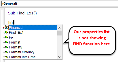
VBA Find
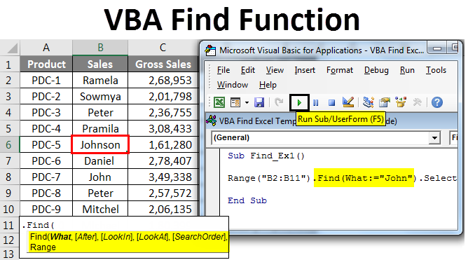
Excel VBA Find Function
Who doesn’t know FIND method in excel? I am sure everybody knows who are dealing with excel worksheets. FIND or popular shortcut key Ctrl + F will find the word or content you are searching for in the entire worksheet as well as in the entire workbook. When you say find means you are finding in cells or ranges isn’t it? Yes, the correct find method is part of the cells or ranges in excel as well as in VBA.
Similarly, in VBA Find, we have an option called FIND function which can help us find the value we are searching for. In this article, I will take you through the methodology of FIND in VBA.
Valuation, Hadoop, Excel, Mobile Apps, Web Development & many more
Formula to Find Function in Excel VBA
In regular excel worksheet, we simply type shortcut key Ctrl + F to find the contents. But in VBA we need to write a function to find the content we are looking for. Ok, let’s look at the FIND syntax then.

I know what is going on in your mind, you are lost by looking at this syntax and you are understanding nothing. But nothing to worry before I explain you the syntax let me introduce you to the regular search box.
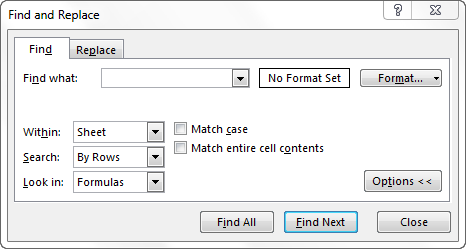
If you observe what is there in regular Ctrl + F, everything is there in VBA Find syntax as well. Now take a look at what each word in syntax says about.
What: Simply what you are searching for. Here we need to mention the content we are searching for.
After: After which cell you want to search for.
LookIn: Where to look for the thing you are searching For example Formulas, Values, or Comments. Parameters are xlFormulas, xlValues, xlComments.
LookAt: Whether you are searching for the whole content or only the part of the content. Parameters are xlWhole, xlPart.
SearchOrder: Are you looking in rows or Columns. xlByRows or xlByColumns.
SearchDirection: Are you looking at the next cell or previous cell. xlNext, xlPrevious.
MatchCase: The content you are searching for is case sensitive or not. True or False.
MatchByte: This is only for double-byte languages. True or False.
SearchFormat: Are you searching by formatting. If you are searching for format then you need to use Application.FindFormat method.
This is the explanation of the syntax of the VBA FIND method. Apart from the first parameter, everything is optional. In the examples section, we will see how to use this FIND method in VBA coding.
How to Use Excel VBA Find Function?
We will learn how to use a VBA Find Excel function with few examples.
VBA Find Function – Example #1
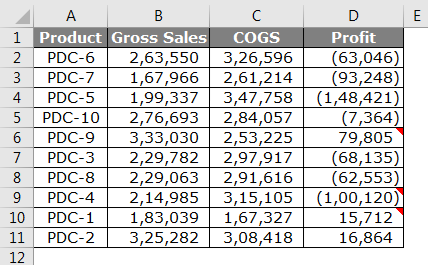
First up let me explain you a simple example of using FIND property and find the content we are looking for. Assume below is the data you have in your excel sheet.
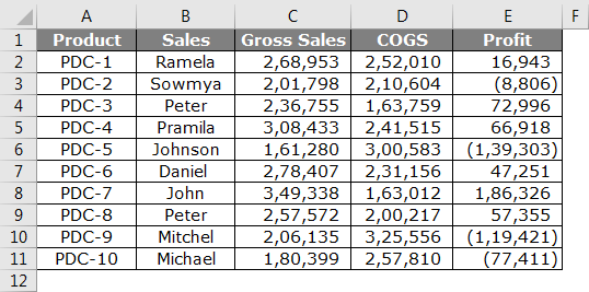
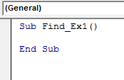
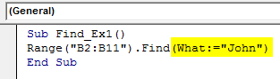
Step 1: From this, I want to find the name John, let’s open a Visual basic and start the coding.
Code:
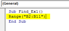
Step 2: Here you cannot start the word FIND, because FIND is part of RANGE property. So, firstly we need to mention where we are looking i.e. Range.
Step 3: So first mention the range where we are looking for. In our example, our range is from B2 to B11.
Code:
Step 4: After mentioning the range put a dot (.) and type FIND. You must see FIND property.
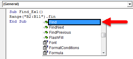
Step 5: Select the FIND property and open the bracket.
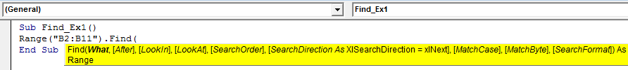
Step 6: Our first argument is what we are searching for. In order to highlight the argument we can pass the argument like this What:=, this would be helpful to identify which parameter we are referring to.
Code:
Step 7: The final part is after finding the word what we want to do. We need to select the word, so pass the argument as .Select.
Code:
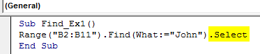
Step 8: Then run this code using F5 key or manually as shown in the figure, so it would select the first found word Johnson which contains a word, John.
VBA Find Function – Example #2
Now I will show you how to find the comment word using the find method. I have data and in three cells I have a comment.
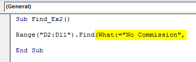
Those cells having red flag has comments in it. From this comment, I want to search the word “No Commission”.
Step 1: Start code with mentioning the Range (“D2:D11”) and put a dot (.) and type Find
Code:
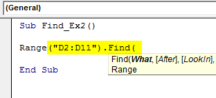
Step 2: In the WHAT argument type the word “No Commission”.
Code:
Step 3: Ignore the After part and select the LookIn part. In LookIn part we are searching this word in comments so select xlComments and then pass the argument as .Select
Code:
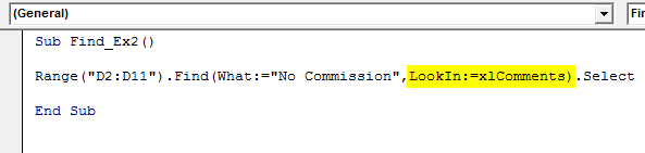
Step 4: Now run this code using F5 key or manually as shown in the figure so it will select the cell which has the comment “No Commission”. In D9 cell we have a mentioned comment.
Deal with Error Values in Excel VBA Find
If the word we are searching for does not find in the range we have supplied VBA code which will return an error like this.
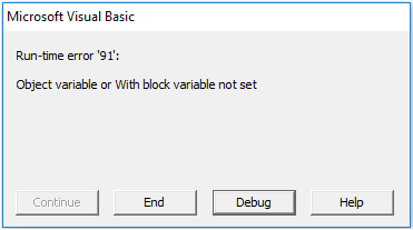
In order to show the user that the value you are searching for is not available, we need the below code.
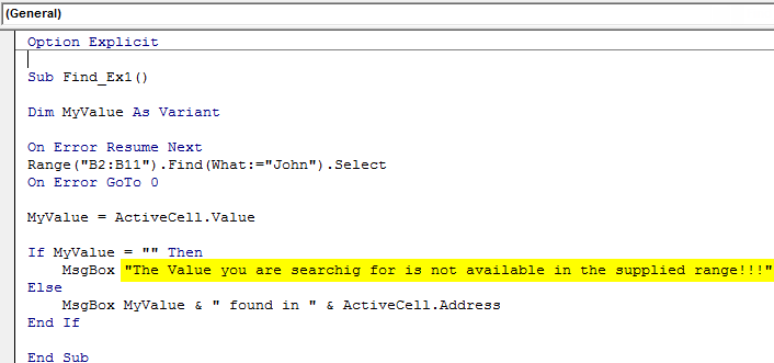
If the above code found value then it shows the value & cell address or else it will show the message as “The Value you are searching for is not available in the supplied range. ”.
Things to Remember
- VBA FIND is part of the RANGE property & you need to use the FIND after selecting the range only.
- In FIND first parameter is mandatory (What) apart from this everything else is optional.
- If you to find the value after specific cell then you can mention the cell in the After parameter of the Find syntax.
Recommended Articles
This has been a guide to VBA Find Function. Here we discussed VBA Find and how to use Excel VBA Find Function along with some practical examples and downloadable excel template. You can also go through our other suggested articles –
All in One Software Development Bundle (600+ Courses, 50+ projects)
Ron de Bruin
Excel Automation
Find value in Range, Sheet or Sheets with VBA
Copy the code in a Standard module of your workbook, if you just started with VBA see this page.
Where do I paste the code that I find on the internet
Find is a very powerful option in Excel and is very useful. Together with the Offset function you can also change cells around the found cell. Below are a few basic examples that you can use to in your own code.
Use Find to select a cell
The examples below will search in column A of a sheet named «Sheet1» for the inputbox value. Change the sheet name or range in the code to your sheet/range.
Tip: You can replace the inputbox with a string or a reference to a cell like this
FindString = «SearchWord»
Or
FindString = Sheets(«Sheet1»).Range(«D1»).Value
This example will select the first cell in the range with the InputBox value.
If you have more then one occurrence of the value this will select the last occurrence.
If you have date’s in column A then this example will select the cell with today’s date. Note : If your dates are formulas it is possible that you must change xlFormulas to xlValues in the example below. If your dates are values xlValues is not always working with some date formats.
Mark cells with the same value in column A in the B column
This example search in Sheets(«Sheet1») in column A for every cell with «ron» and use Offset to mark the cell in the column to the right. Note: you can add more values to the array MyArr.
Color cells with the same value in a Range, worksheet or all worksheets
This example color all cells in the range Sheets(«Sheet1»).Range(«B1:D100») with «ron». See the comments in the code if you want to use all cells on the worksheet. I use the color index in this example to give all cells with «ron» the color 3 (normal this is red)
Tip: For changing the Font color see the example lines below the macros.
Example for all worksheets in the workbook
Change the Font color instead of the Interior color
‘Change the fill color to «no fill» in all cells
.Interior.ColorIndex = xlColorIndexNone
‘Change the font in the column to Automatic
.Font.ColorIndex = 0
Rng.Interior.ColorIndex = myColor(I)
With
Rng.Font.ColorIndex = myColor(I)
Copy cells to another sheet with Find
The example below will copy all cells with a E-Mail Address in the range Sheets(«Sheet1»).Range(«A1:E100») to a new worksheet in your workbook. Note: I use xlPart in the code instead of xlWhole to find each cell with a @ character.
If you only want to replace values in your worksheet then you can use Replace manual (Ctrl+h) or use Replace in VBA. The code below replace ron for dave in the whole worksheet. Change xlPart to xlWhole if you only want to replace cells with only ron.
Excel VBA FIND Function (& how to handle if value NOT found)
Doing a CTRL + F on Excel to find a partial or exact match in the cell values, formulas or comments gives you a result almost instantly. In fact, it might even be faster to use this instead looping through multiple cells or rows in VBA. MS Excel’s FIND method automates this process without looping.

Arguments needed
MSDN.Microsoft.com gives you a summary of parameters and arguments for MS Excel functions.

This means that the FIND function can be used on a Range object on the worksheet. It is used in the format:
Expression.Find(What, After, LookIn, LookAt, SearchOrder, SearchDirection, MatchCase, MatchByte, SearchFormat)
The answer should be saved as a Range object, so the Set keyword should be used when using the FIND() method.

The only required parameter is what is being looked for and the rest is optional. The optional parameters have default values corresponding to whatever was selected last on a manual search. For example, if the user specified to search within the Excel comments in the last manual search, the FIND() function will then only look at Excel comments if a LookIn value is not specified—which may or may not be how the FIND() function is expected to run. Because of this, it’s recommended to specify the parameters listed below to make sure the function runs in a way that is expected:
- LookIn – decides where the variable is to be found (xlFormulas, xlValues, xlNotes)
- LookAt – full or partial match (xlWhole, or xlPart)
- MatchCase – TRUE to make the search case sensitive. Default value is FALSE
- After – useful when looking for multiple matches since it specifies the cell after which the search should begin
The FIND() method to find one match
In this example, the button One Match should display the corresponding article code from the given data table depending on what company code the user selects.

- Bring up the Visual Basic editor (ALT + F11).
- Create a new module by going to Insert > Module.
- Create a new Subprocedure

Find the company id match
1. Write the variable to keep the result of the FIND() function. In this example, the variable CompId is used and is written as:
Dim CompId As Range
- What:=Range(“B3”).Value – the value to be searched
- LookIn:=xlValues – looks at the cell values
- LookAt:=xlWhole – full match

Note: cells.Find can be used if you want to search the entire worksheet or don’t know where the company Id column is.
Activate the watch window
Activating the Watch Window (under View) helps you identify what steps are missing in the code. Highlight the variable to be watched and drag it to the watch window. Run the code (or press F8).

The watch window shows the value of CompId, which is the match of the Company Id selected by the user. To better understand exactly which cell it is pointing to, change the Expression from CompId to CompId.Address. This will then give you $A$8, which corresponds to the address of the match.

Display the equivalent Article Code
Since the corresponding Article Code should be displayed in cell C3, set up the formula to get the Article code which is 4 columns to the right of the company id on the data table using the Offset function:
This now becomes:

Note: A 0 can be used for the [RowOffset] parameter, or left blank and skipped by the symbol “,”
Address values that are not found on the table
When the selected Company Id is not found on the table, the watch window shows an error in CompId.Address because the CompId.Value is nothing and is invalid for the Range data type.


An IF statement should be added to address such cases. In VBA, the keyword NOT is used often since it is usually easier to specify what something isn’t, than what something is. In this case, the result can either be nothing or specific ranges. When it is nothing, you can alert the user with a message box indicating so. The IF statement then becomes:
If Not CompId is Nothing Then
Msgbox “Company not found!”

However, while it displays the message box when the company id is not found, the value in cell C3 retains the result of the previous search. Make sure that the macro deletes the contents of the cell before it runs the rest of the code:

Assign the macro to the button
Right click on the button > Assign macro. Select the macro name.