
I have two columns in Excel, and I want to find (preferably highlight) the items that are in column B but not in column A.
What’s the quickest way to do this?
![]()
Excellll
12.5k11 gold badges50 silver badges78 bronze badges
asked Dec 10, 2009 at 18:44
![]()
- Select the list in column A
- Right-Click and select Name a Range…
- Enter «ColumnToSearch»
- Click cell C1
- Enter this formula:
=MATCH(B1,ColumnToSearch,0) - Drag the formula down for all items in B
If the formula fails to find a match, it will be marked #N/A, otherwise it will be a number.
If you’d like it to be TRUE for match and FALSE for no match, use this formula instead:
=ISNUMBER(MATCH(B1,ColumnToSearch,0))
If you’d like to return the unfound value and return empty string for found values
=IF(ISNUMBER(MATCH(B1,ColumnToSearch,0)),"",B1)
![]()
answered Dec 10, 2009 at 19:01
![]()
devuxerdevuxer
3,9316 gold badges31 silver badges33 bronze badges
6
Here’s a quick-and-dirty method.
Highlight Column B and open Conditional Formatting.
Pick Use a formula to determine which cells to highlight.
Enter the following formula then set your preferred format.
=countif(A:A,B1)=0
![]()
Excellll
12.5k11 gold badges50 silver badges78 bronze badges
answered May 9, 2011 at 16:18
![]()
EllesaEllesa
10.8k2 gold badges38 silver badges52 bronze badges
2
Select the two columns. Go to Conditional Formatting and select Highlight Cell Rules. Select Duplicate values. When you get to the next step you can change it to unique values. I just did it and it worked for me.
answered Apr 16, 2015 at 20:02
![]()
DOB DOB
2813 silver badges2 bronze badges
4
Took me forever to figure this out but it’s very simple. Assuming data begins in A2 and B2 (for headers) enter this formula in C2:
=MATCH(B2,$A$2:$A$287,0)
Then click and drag down.
A cell with #N/A means that the value directly next to it in column B does not show up anywhere in the entire column A.
Please note that you need to change $A$287 to match your entire search array in Column A. For instance if your data in column A goes down for 1000 entries it should be $A$1000.
![]()
n.st
1,8781 gold badge17 silver badges30 bronze badges
answered Dec 6, 2013 at 20:43
![]()
brentonbrenton
1711 silver badge2 bronze badges
1
See my array formula answer to listing A not found in B here:
=IFERROR(INDEX($A$2:$A$1999,MATCH(0,IFERROR(MATCH($A$2:$A$1999,$B$2:$B$399,0),COUNTIF($C$1:$C1,$A$2:$A$1999)),0)),»»)
Comparing two columns of names and returning missing names
![]()
C. Ross
6,06416 gold badges60 silver badges82 bronze badges
answered Oct 21, 2011 at 14:02
![]()
1
My requirements was not to highlight but to show all values except that are duplicates amongst 2 columns. I took help of @brenton’s solution and further improved to show the values so that I can use the data directly:
=IF(ISNA(MATCH(B2,$A$2:$A$2642,0)), A2, "")
Copy this in the first cell of the 3rd column and apply the formula through out the column so that it will list all items from column B there are not listed in column A.
answered Feb 24, 2014 at 11:10
![]()
1
Thank you to those who have shared their answers. Because of your solutions, I was able to make my way to my own.
In my version of this question, I had two columns to compare — a full graduating class (Col A) and a subset of that graduating class (Col B). I wanted to be able to highlight in the full graduating class those students who were members of the subset.
I put the following formula into a third column:
=if(A2=LOOKUP(A2,$B$2:$B$91),1100,0)
This coded most of my students, though it yielded some errors in the first few rows of data.
answered Sep 11, 2014 at 13:25
![]()
in C1 write =if(A1=B1 , 0, 1). Then in Conditional formatting, select Data bars or Color scales. It’s the easiest way.
![]()
Jawa
3,60913 gold badges31 silver badges36 bronze badges
answered Feb 16, 2015 at 9:52
![]()
Summary
This step-by-step article describes how to find data in a table (or range of cells) by using various built-in functions in Microsoft Excel. You can use different formulas to get the same result.
Create the Sample Worksheet
This article uses a sample worksheet to illustrate Excel built-in functions. Consider the example of referencing a name from column A and returning the age of that person from column C. To create this worksheet, enter the following data into a blank Excel worksheet.
You will type the value that you want to find into cell E2. You can type the formula in any blank cell in the same worksheet.
|
A |
B |
C |
D |
E |
||
|
1 |
Name |
Dept |
Age |
Find Value |
||
|
2 |
Henry |
501 |
28 |
Mary |
||
|
3 |
Stan |
201 |
19 |
|||
|
4 |
Mary |
101 |
22 |
|||
|
5 |
Larry |
301 |
29 |
Term Definitions
This article uses the following terms to describe the Excel built-in functions:
|
Term |
Definition |
Example |
|
Table Array |
The whole lookup table |
A2:C5 |
|
Lookup_Value |
The value to be found in the first column of Table_Array. |
E2 |
|
Lookup_Array |
The range of cells that contains possible lookup values. |
A2:A5 |
|
Col_Index_Num |
The column number in Table_Array the matching value should be returned for. |
3 (third column in Table_Array) |
|
Result_Array |
A range that contains only one row or column. It must be the same size as Lookup_Array or Lookup_Vector. |
C2:C5 |
|
Range_Lookup |
A logical value (TRUE or FALSE). If TRUE or omitted, an approximate match is returned. If FALSE, it will look for an exact match. |
FALSE |
|
Top_cell |
This is the reference from which you want to base the offset. Top_Cell must refer to a cell or range of adjacent cells. Otherwise, OFFSET returns the #VALUE! error value. |
|
|
Offset_Col |
This is the number of columns, to the left or right, that you want the upper-left cell of the result to refer to. For example, «5» as the Offset_Col argument specifies that the upper-left cell in the reference is five columns to the right of reference. Offset_Col can be positive (which means to the right of the starting reference) or negative (which means to the left of the starting reference). |
Functions
LOOKUP()
The LOOKUP function finds a value in a single row or column and matches it with a value in the same position in a different row or column.
The following is an example of LOOKUP formula syntax:
=LOOKUP(Lookup_Value,Lookup_Vector,Result_Vector)
The following formula finds Mary’s age in the sample worksheet:
=LOOKUP(E2,A2:A5,C2:C5)
The formula uses the value «Mary» in cell E2 and finds «Mary» in the lookup vector (column A). The formula then matches the value in the same row in the result vector (column C). Because «Mary» is in row 4, LOOKUP returns the value from row 4 in column C (22).
NOTE: The LOOKUP function requires that the table be sorted.
For more information about the LOOKUP function, click the following article number to view the article in the Microsoft Knowledge Base:
How to use the LOOKUP function in Excel
VLOOKUP()
The VLOOKUP or Vertical Lookup function is used when data is listed in columns. This function searches for a value in the left-most column and matches it with data in a specified column in the same row. You can use VLOOKUP to find data in a sorted or unsorted table. The following example uses a table with unsorted data.
The following is an example of VLOOKUP formula syntax:
=VLOOKUP(Lookup_Value,Table_Array,Col_Index_Num,Range_Lookup)
The following formula finds Mary’s age in the sample worksheet:
=VLOOKUP(E2,A2:C5,3,FALSE)
The formula uses the value «Mary» in cell E2 and finds «Mary» in the left-most column (column A). The formula then matches the value in the same row in Column_Index. This example uses «3» as the Column_Index (column C). Because «Mary» is in row 4, VLOOKUP returns the value from row 4 in column C (22).
For more information about the VLOOKUP function, click the following article number to view the article in the Microsoft Knowledge Base:
How to Use VLOOKUP or HLOOKUP to find an exact match
INDEX() and MATCH()
You can use the INDEX and MATCH functions together to get the same results as using LOOKUP or VLOOKUP.
The following is an example of the syntax that combines INDEX and MATCH to produce the same results as LOOKUP and VLOOKUP in the previous examples:
=INDEX(Table_Array,MATCH(Lookup_Value,Lookup_Array,0),Col_Index_Num)
The following formula finds Mary’s age in the sample worksheet:
=INDEX(A2:C5,MATCH(E2,A2:A5,0),3)
The formula uses the value «Mary» in cell E2 and finds «Mary» in column A. It then matches the value in the same row in column C. Because «Mary» is in row 4, the formula returns the value from row 4 in column C (22).
NOTE: If none of the cells in Lookup_Array match Lookup_Value («Mary»), this formula will return #N/A.
For more information about the INDEX function, click the following article number to view the article in the Microsoft Knowledge Base:
How to use the INDEX function to find data in a table
OFFSET() and MATCH()
You can use the OFFSET and MATCH functions together to produce the same results as the functions in the previous example.
The following is an example of syntax that combines OFFSET and MATCH to produce the same results as LOOKUP and VLOOKUP:
=OFFSET(top_cell,MATCH(Lookup_Value,Lookup_Array,0),Offset_Col)
This formula finds Mary’s age in the sample worksheet:
=OFFSET(A1,MATCH(E2,A2:A5,0),2)
The formula uses the value «Mary» in cell E2 and finds «Mary» in column A. The formula then matches the value in the same row but two columns to the right (column C). Because «Mary» is in column A, the formula returns the value in row 4 in column C (22).
For more information about the OFFSET function, click the following article number to view the article in the Microsoft Knowledge Base:
How to use the OFFSET function
Need more help?
Want more options?
Explore subscription benefits, browse training courses, learn how to secure your device, and more.
Communities help you ask and answer questions, give feedback, and hear from experts with rich knowledge.
![]()

What?
A quick note on how to compare two columns for values that are not found in another. I have a column with old values, and now that I have a new list, I want a quick way to see what values are in the old column and which ones are new…
Why?
Consider the 3 following columns in an Excel spreadsheet:
copyraw
Old       New       Exists in Old?
--------- --------- --------------
123456    234567
234567    345678
345678    456789
567890    597890
- Old New Exists in Old?
- 123456 234567
- 234567 345678
- 345678 456789
- 567890 597890
I want the third column to say whether this is new or not.
How?
I found this in a StackExchange site:
Method #1
copyraw
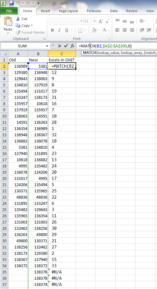
=MATCH(B2, $A$2:$A$100, 0)

-- Check whether value in B2 exists in range of A2:A100.
-- Returns the index of column A in which the B2 value was found.
-- Returns #N/A for a value which is NOT in column A.
- =MATCH(B2, $A$2:$A$100, 0)
Drag the formula in B2 down all the list as per the following screenshot. A value equal to «#N/A» means the value was NOT found in column A.
Method #2
Be careful with this one because if you copy the formula down, it may automatically modify the range. So the formula in the first row will be
=COUNTIF(A2:A100, B2)
but the formula in the second row will be
=COUNTIF(A3:A101, B3)
:
copyraw
=COUNTIF(A2:A100, B2)

-- Returns 1 if value in B2 was found in range A2:A100
-- Returns 0 if value in B2 was not found in range A.
- =COUNTIF(A2:A100, B2)
Category: Excel :: Article: 551
Related Articles
-
Select unique values in Microsoft Excel column
(6114)
(Excel)
Thought I’d put a quick note here, I tried a fair few solutions that didn’t work and then found this hidden away in a…
-
Blank columns issue when exporting to Excel (Data Only) from Crystal Reports
(46606)
Joel Lipman
(Excel)
Following up on my article on correcting disappearing headers, a further issue with our web-report is that even an export to…
-
MS Excel — Split Workbook into separate files per sheet
(2644)
Joel Lipman
(Excel)
What?
This article serves to explain how to split a spreadsheet consisting of multiple sheets into separate files per… -
Excel PivotTable Filter List Ordering
(16756)
Joel Lipman
(Excel)
So I googled this for a while and there are a lot of solutions out there, none of which applied to what we meant and…
-
Import Excel CSV file as JavaScript array
(1880)
Joel Lipman
(Excel)
What I have:
A CSV file exported from Excel along with double-quoteslabel1,label2
item1a,item2a
item1c,»item2c,c»
item1b,item2bWhat I want:
To read the file… -
Excel: Find values in one column that are not in another
(17799)
Joel Lipman
(Excel)
What?
A quick note on how to compare two columns for values that are not found in another. I have a column with old… -
Convert Decimal (Person Days) to Time in Excel
(6164)
Joel Lipman
(Excel)
What?
We have an excel spreadsheet which reports against a mySQL database and reads time spent on projects by IT…
Joes Revolver Map
Joes Word Cloud
Accreditation
Donate & Support
If you like my content, and would like to support this sharing site, feel free to donate using a method below:
Paypal:

Bitcoin:

bc1qjtp4l4ra452wzvuk9a45yfj82zkahsyy2z379y

There are multiple ways of using Excel to check if a value exists in another column such as manually using the ribbon, using a MATCH formula or using a VLOOKUP formula.
Additionally there are clever things we can do to handle dynamically expanding datasets such as by defining tables and complex ranges. But if you don’t want to know the ins and outs, and just need a quick and dirty formula to return ‘true’ or ‘false’, you can use this.
Using Excel to Check if a Value Exists in Another Column
Here we are simply checking if the value in cell A2 exists in any cell in column B (except the first row, which we assume is a header).
=IF(ISERROR(VLOOKUP(A2,$B$2:$B$1001,1,FALSE)),FALSE,TRUE)Please note that this formula has a couple of assumptions:
- It excludes the first row of data from the lookup, and assumes that this row is a header. If your data does not have headers, change it to:
=IF(ISERROR(VLOOKUP(A1,$B$1:$B$1000,1,FALSE)),FALSE,TRUE) - It also assumes your lookup data only has 1000 rows (of course it would need to iterate through 1001 rows if it contained a header!). If your dataset has more rows of data, you would also need to adjust this value.


Explanation
The COUNTIF function counts cells that meet criteria, returning the number of occurrences found. If no cells meet criteria, COUNTIF returns zero. You can use behavior directly inside an IF statement to mark values that have a zero count (i.e. values that are missing). In the example shown, the formula in G6 is:
=IF(COUNTIF(list,F6),"OK","Missing")
where «list» is a named range that corresponds to the range B6:B11.
The IF function requires a logical test to return TRUE or FALSE. In this case, the COUNTIF function performs the logical test. If the value is found in list, COUNTIF returns a number directly to the IF function. This result could be any number… 1, 2, 3, etc.
The IF function will evaluate any number as TRUE, causing IF to return «OK». If the value is not found in list, COUNTIF returns zero (0), which evaluates as FALSE, and IF returns «Missing».
Alternative with MATCH
You can also test for missing values using the MATCH function. MATCH finds the position of an item in a list and will return the #N/A error when a value is not found. You can use this behavior to build a formula that returns «Missing» or «OK» by testing the result of MATCH with the ISNA function. ISNA returns TRUE only when it receives the #N/A error.
To use MATCH as shown in the example above, the formula is:
=IF(ISNA(MATCH(F6,list,0)),"Missing","OK")

Note that MATCH must be configured for exact match. To do this, make sure the third argument is zero or FALSE.
Alternative with VLOOKUP
Since VLOOKUP also returns an #N/A error when a value isn’t round, you can build a formula with VLOOKUP that works the same as the MATCH option. As with MATCH, you must configure VLOOKUP to use exact match, then test the result with ISNA. Also note that we only give VLOOKUP a single column (column B) for the table array.
