
Summary
This step-by-step article describes how to find data in a table (or range of cells) by using various built-in functions in Microsoft Excel. You can use different formulas to get the same result.
Create the Sample Worksheet
This article uses a sample worksheet to illustrate Excel built-in functions. Consider the example of referencing a name from column A and returning the age of that person from column C. To create this worksheet, enter the following data into a blank Excel worksheet.
You will type the value that you want to find into cell E2. You can type the formula in any blank cell in the same worksheet.
|
A |
B |
C |
D |
E |
||
|
1 |
Name |
Dept |
Age |
Find Value |
||
|
2 |
Henry |
501 |
28 |
Mary |
||
|
3 |
Stan |
201 |
19 |
|||
|
4 |
Mary |
101 |
22 |
|||
|
5 |
Larry |
301 |
29 |
Term Definitions
This article uses the following terms to describe the Excel built-in functions:
|
Term |
Definition |
Example |
|
Table Array |
The whole lookup table |
A2:C5 |
|
Lookup_Value |
The value to be found in the first column of Table_Array. |
E2 |
|
Lookup_Array |
The range of cells that contains possible lookup values. |
A2:A5 |
|
Col_Index_Num |
The column number in Table_Array the matching value should be returned for. |
3 (third column in Table_Array) |
|
Result_Array |
A range that contains only one row or column. It must be the same size as Lookup_Array or Lookup_Vector. |
C2:C5 |
|
Range_Lookup |
A logical value (TRUE or FALSE). If TRUE or omitted, an approximate match is returned. If FALSE, it will look for an exact match. |
FALSE |
|
Top_cell |
This is the reference from which you want to base the offset. Top_Cell must refer to a cell or range of adjacent cells. Otherwise, OFFSET returns the #VALUE! error value. |
|
|
Offset_Col |
This is the number of columns, to the left or right, that you want the upper-left cell of the result to refer to. For example, «5» as the Offset_Col argument specifies that the upper-left cell in the reference is five columns to the right of reference. Offset_Col can be positive (which means to the right of the starting reference) or negative (which means to the left of the starting reference). |
Functions
LOOKUP()
The LOOKUP function finds a value in a single row or column and matches it with a value in the same position in a different row or column.
The following is an example of LOOKUP formula syntax:
=LOOKUP(Lookup_Value,Lookup_Vector,Result_Vector)
The following formula finds Mary’s age in the sample worksheet:
=LOOKUP(E2,A2:A5,C2:C5)
The formula uses the value «Mary» in cell E2 and finds «Mary» in the lookup vector (column A). The formula then matches the value in the same row in the result vector (column C). Because «Mary» is in row 4, LOOKUP returns the value from row 4 in column C (22).
NOTE: The LOOKUP function requires that the table be sorted.
For more information about the LOOKUP function, click the following article number to view the article in the Microsoft Knowledge Base:
How to use the LOOKUP function in Excel
VLOOKUP()
The VLOOKUP or Vertical Lookup function is used when data is listed in columns. This function searches for a value in the left-most column and matches it with data in a specified column in the same row. You can use VLOOKUP to find data in a sorted or unsorted table. The following example uses a table with unsorted data.
The following is an example of VLOOKUP formula syntax:
=VLOOKUP(Lookup_Value,Table_Array,Col_Index_Num,Range_Lookup)
The following formula finds Mary’s age in the sample worksheet:
=VLOOKUP(E2,A2:C5,3,FALSE)
The formula uses the value «Mary» in cell E2 and finds «Mary» in the left-most column (column A). The formula then matches the value in the same row in Column_Index. This example uses «3» as the Column_Index (column C). Because «Mary» is in row 4, VLOOKUP returns the value from row 4 in column C (22).
For more information about the VLOOKUP function, click the following article number to view the article in the Microsoft Knowledge Base:
How to Use VLOOKUP or HLOOKUP to find an exact match
INDEX() and MATCH()
You can use the INDEX and MATCH functions together to get the same results as using LOOKUP or VLOOKUP.
The following is an example of the syntax that combines INDEX and MATCH to produce the same results as LOOKUP and VLOOKUP in the previous examples:
=INDEX(Table_Array,MATCH(Lookup_Value,Lookup_Array,0),Col_Index_Num)
The following formula finds Mary’s age in the sample worksheet:
=INDEX(A2:C5,MATCH(E2,A2:A5,0),3)
The formula uses the value «Mary» in cell E2 and finds «Mary» in column A. It then matches the value in the same row in column C. Because «Mary» is in row 4, the formula returns the value from row 4 in column C (22).
NOTE: If none of the cells in Lookup_Array match Lookup_Value («Mary»), this formula will return #N/A.
For more information about the INDEX function, click the following article number to view the article in the Microsoft Knowledge Base:
How to use the INDEX function to find data in a table
OFFSET() and MATCH()
You can use the OFFSET and MATCH functions together to produce the same results as the functions in the previous example.
The following is an example of syntax that combines OFFSET and MATCH to produce the same results as LOOKUP and VLOOKUP:
=OFFSET(top_cell,MATCH(Lookup_Value,Lookup_Array,0),Offset_Col)
This formula finds Mary’s age in the sample worksheet:
=OFFSET(A1,MATCH(E2,A2:A5,0),2)
The formula uses the value «Mary» in cell E2 and finds «Mary» in column A. The formula then matches the value in the same row but two columns to the right (column C). Because «Mary» is in column A, the formula returns the value in row 4 in column C (22).
For more information about the OFFSET function, click the following article number to view the article in the Microsoft Knowledge Base:
How to use the OFFSET function
Need more help?
Want more options?
Explore subscription benefits, browse training courses, learn how to secure your device, and more.
Communities help you ask and answer questions, give feedback, and hear from experts with rich knowledge.
Transcript
In this lesson, we’ll look at how to find things in Excel.
Let’s take a look.
To find a value in Excel, use the Find and Replace dialog box. You can access this dialog using the keyboard shortcut control-F, or, by using the Find and Select menu at the far right of the Home tab on the ribbon.
Let’s try looking for the name Ann. Nothing happens until we click the Find Next button. Then, each time we click, Excel finds another match.
Note that Excel finds other names that contain Ann as well—Annie, Ann, Danny, and then Hannah. If we continue clicking Find Next, Excel will eventually return to the first match.
By default, Excel searches left to right, first through rows, then columns. You can hold down the shift key when you press «Find Next» to move backwards.
Now let’s review the Find options.
The first option allows you to restrict the search to the current worksheet, or expand it to include the entire workbook. If we select workbook, Excel will now find matches on Sheet 2.
The «search» option determines the order that Excel looks through cells. The default is «By Rows.» If we switch to «By Columns,» Excel will find all matches in one column before moving on to the next column.
There is also an option to search Formulas, Values, and Comments. We’ll look at these in a future lesson.
If we enable «Match case,» Excel treats case as important and only finds values that begin with a capital A.
If we enable «Match entire cell contents,» Excel will only find cells where the value is exactly Ann. This is a good way to find only the name Ann.
With the Find dialog closed, you can still find things with the keyboard shortcut Shift F4. Excel will use the current Find settings and select the next match.
Finally, it’s important to understand that if you have more than one cell selected, Excel will search only in the current selection. For example, if we select just a subset of our table, Excel will only search in that selection.
However, if you switch «Within» to «Workbook,» Excel will drop the current selection and search all cells. At this point, you can switch back to Worksheet to search only the current worksheet.
|
sku144  Пользователь Сообщений: 19 |
#1 20.01.2015 14:51:01 Привет. Никак не могу понять, как через Cells.Find найти значение в ячейке А1. Какой параметр надо указать в Cells.Find(After:=), чтобы поиск находил значнеие в А1 независимо от выделенной ячейки. Попробовал три возможных известных мне варианта, ни один не помогает. Вот для примера макрос (лучше запускать пошагово через F8), который не может найти единицу в левом верхнем углу
|
||
|
Юрий М  Модератор Сообщений: 60570 Контакты см. в профиле |
#2 20.01.2015 15:00:03
|
||
|
sku144 Пользователь Сообщений: 19 |
#3 20.01.2015 15:43:52
Спасибо, Юрий М , а как предложенной конструкцией выделить найденное? .Select или .Activate не работает И можно ли решить поставленную задачу через Cells.Find |
||
|
Юрий М Модератор Сообщений: 60570 Контакты см. в профиле |
#4 20.01.2015 15:45:56
Всё работает:
|
||||
|
sku144 Пользователь Сообщений: 19 |
аа, «Rng.Select», я его вставлял после «Range(«A1» Юрий М , спасибо, но, как бы то ни было, вопрос про Cells.Find актулаен. Изменено: sku144 — 20.01.2015 16:30:27 |
|
Максим Зеленский  Пользователь Сообщений: 4646 Microsoft MVP |
#6 20.01.2015 16:30:20
а в чем отличие Cells.Find от Range.Find? Cells.Find — поиск во всех ячейках, а Range(«A1» Изменено: Максим Зеленский — 20.01.2015 16:40:59 F1 творит чудеса |
||
|
Юрий М Модератор Сообщений: 60570 Контакты см. в профиле |
#7 20.01.2015 16:31:26 Не понимаю, почему не устраивает предложенный вариант… Но если уж так принципиально, то вот что записывает рекордер:
|
||
|
sku144 Пользователь Сообщений: 19 |
Юрий М
, Если поставить курсор в ячейку А1, то будет выделена другая ячейка со значением 1, в то время, как нам надо подсветить первое встреченное, а не второе. Максим Зеленский , мы ищем по всем ячейкам на листе. когда курсор находится на А1, Cells.Find показывает второе найденное знчение в какой-то другой ячейке Изменено: sku144 — 20.01.2015 16:48:35 |
|
Юрий М Модератор Сообщений: 60570 Контакты см. в профиле |
1. Добавьте проверку адреса ячейки. |
|
Alexander88  Пользователь Сообщений: 400 |
#10 20.01.2015 16:48:11 Так попробуйте
|
||
|
sku144 Пользователь Сообщений: 19 |
Имеем три единицы на листе — на А1, на B2 и на C1 Alexander88 , почему-то находит на C1 игнорируя А1. То же самое, как если бы мы не указывали где искать. Майкрософт говорит про аргумент After: Юрий М , все мы знаем про TMTOWTDI , и то что вы предложили — безусловно хорошая альтернатива. можно даже забить на первую ячейку, и перед поиском тупо проверить ее IFом на наличие искомого значения. Но почему, черт побери, почему Cells.Find, который нам так любезно предлагает макрорекордер, не может захватывать первую ячейку из диапазона? Изменено: sku144 — 20.01.2015 17:58:40 |
|
Johny Пользователь Сообщений: 2737 |
#12 20.01.2015 16:57:59
Разница есть. Зависит от того, в каком контексте используется «Cells». Просто «Cells» — это все ячейки активного листа, а Range(«A1:F20»).Cells — это ячейки именно диапазона A1:F20. There is no knowledge that is not power |
||
|
Юрий М Модератор Сообщений: 60570 Контакты см. в профиле |
#13 20.01.2015 17:01:51
Установите диапазон и ищите в нём)) |
||
|
Alexander88 Пользователь Сообщений: 400 |
#14 20.01.2015 17:03:10 Не понимаю для чего это нужно..
Изменено: Alexander88 — 20.01.2015 17:15:09 |
||
|
V Пользователь Сообщений: 5018 |
#15 20.01.2015 17:16:43
|
||
|
sku144 Пользователь Сообщений: 19 |
Alexander88
, а в чем смысл извращения, когда мы говорим ищи во всях ячейках на листе, а потом ограничиваем поиск? А диапазона точного, я кстати, не знаю, да и не хочу лишним кодом утруждать эксель выискивать нужный диапазон, когда надо всего лишь понять, как правильно прописать значение аргументов для Cells.Find |
|
The_Prist  Пользователь Сообщений: 14181 Профессиональная разработка приложений для MS Office |
#17 20.01.2015 17:18:41 Итак. По умолчанию поиск идет после активной ячейки. Если указать все ячейки листа, то первая ячейка диапазона будет проигнорирована(если делать из VBA), т.к. будет считаться, что именно она является активной и поиск должен быть осуществлен после нее. Принудительная активация ячейки тоже не спасет. Самое простое это добавить проверку наличия искомого значения в первой ячейке.
Даже самый простой вопрос можно превратить в огромную проблему. Достаточно не уметь формулировать вопросы… |
||
|
sku144 Пользователь Сообщений: 19 |
The_Prist
, да, такой вариант я предлагал уже выше, и, видимо, это единственно возможный вариант с этим грешным способом, спасибо. |
|
Максим Зеленский Пользователь Сообщений: 4646 Microsoft MVP |
#19 20.01.2015 17:21:49
да это я понял. просто никак не мог понять, что хочет автор. Хотел одновременно найти только в А1 и при этом искать на всем листе. После следующих постов стало понятнее F1 творит чудеса |
||
|
Alexander88 Пользователь Сообщений: 400 |
#20 20.01.2015 17:27:41 Я понял, что нужно искать с первой ячейки.. Find
Изменено: Alexander88 — 20.01.2015 17:38:56 |
||
|
sku144 Пользователь Сообщений: 19 |
#21 20.01.2015 17:38:52 Alexander88
, да, вот оно решение, СПАСИБО! |

Поиск какого-либо значения в ячейках Excel довольно часто встречающаяся задача при программировании какого-либо макроса. Решить ее можно разными способами. Однако, в разных ситуациях использование того или иного способа может быть не оправданным. В данной статье я рассмотрю 2 наиболее распространенных способа.
Поиск перебором значений
Довольно простой в реализации способ. Например, найти в колонке «A» ячейку, содержащую «123» можно примерно так:
Sheets("Данные").Select
For y = 1 To Cells.SpecialCells(xlLastCell).Row
    If Cells(y, 1) = "123" Then
        Exit For
    End If
Next y
MsgBox "Нашел в строке: " + CStr(y)
Минусами этого так сказать «классического» способа являются: медленная работа и громоздкость. А плюсом является его гибкость, т.к. таким способом можно реализовать сколь угодно сложные варианты поиска с различными вычислениями и т.п.
Поиск функцией Find
Гораздо быстрее обычного перебора и при этом довольно гибкий. В простейшем случае, чтобы найти в колонке A ячейку, содержащую «123» достаточно такого кода:
Sheets("Данные").Select
Set fcell = Columns("A:A").Find("123")
If Not fcell Is Nothing Then
    MsgBox "Нашел в строке: " + CStr(fcell.Row)
End If
Вкратце опишу что делают строчки данного кода:
1-я строка: Выбираем в книге лист «Данные»;
2-я строка: Осуществляем поиск значения «123» в колонке «A», результат поиска будет в fcell;
3-я строка: Если удалось найти значение, то fcell будет содержать Range-объект, в противном случае — будет пустой, т.е. Nothing.
Полностью синтаксис оператора поиска выглядит так:
Find(What, After, LookIn, LookAt, SearchOrder, SearchDirection, MatchCase, MatchByte, SearchFormat)
What — Строка с текстом, который ищем или любой другой тип данных Excel
After — Ячейка, после которой начать поиск. Обратите внимание, что это должна быть именно единичная ячейка, а не диапазон. Поиск начинается после этой ячейки, а не с нее. Поиск в этой ячейке произойдет только когда весь диапазон будет просмотрен и поиск начнется с начала диапазона и до этой ячейки включительно.
LookIn — Тип искомых данных. Может принимать одно из значений: xlFormulas (формулы), xlValues (значения), или xlNotes (примечания).
LookAt — Одно из значений: xlWhole (полное совпадение) или xlPart (частичное совпадение).
SearchOrder — Одно из значений: xlByRows (просматривать по строкам) или xlByColumns (просматривать по столбцам)
SearchDirection — Одно из значений: xlNext (поиск вперед) или xlPrevious (поиск назад)
MatchCase — Одно из значений: True (поиск чувствительный к регистру) или False (поиск без учета регистра)
MatchByte — Применяется при использовании мультибайтных кодировок: True (найденный мультибайтный символ должен соответствовать только мультибайтному символу) или False (найденный мультибайтный символ может соответствовать однобайтному символу)
SearchFormat — Используется вместе с FindFormat. Сначала задается значение FindFormat (например, для поиска ячеек с курсивным шрифтом так: Application.FindFormat.Font.Italic = True), а потом при использовании метода Find указываем параметр SearchFormat = True. Если при поиске не нужно учитывать формат ячеек, то нужно указать SearchFormat = False.
Чтобы продолжить поиск, можно использовать FindNext (искать «далее») или FindPrevious (искать «назад»).
Примеры поиска функцией Find
Пример 1: Найти в диапазоне «A1:A50» все ячейки с текстом «asd» и поменять их все на «qwe»
With Worksheets(1).Range("A1:A50")
  Set c = .Find("asd", LookIn:=xlValues)
  Do While Not c Is Nothing
    c.Value = "qwe"
    Set c = .FindNext(c)
  Loop
End With
Обратите внимание: Когда поиск достигнет конца диапазона, функция продолжит искать с начала диапазона. Таким образом, если значение найденной ячейки не менять, то приведенный выше пример зациклится в бесконечном цикле. Поэтому, чтобы этого избежать (зацикливания), можно сделать следующим образом:
Пример 2: Правильный поиск значения с использованием FindNext, не приводящий к зацикливанию.
With Worksheets(1).Range("A1:A50")
  Set c = .Find("asd", lookin:=xlValues)
  If Not c Is Nothing Then
    firstResult = c.Address
    Do
      c.Font.Bold = True
      Set c = .FindNext(c)
      If c Is Nothing Then Exit Do
    Loop While c.Address <> firstResult
  End If
End With
В ниже следующем примере используется другой вариант продолжения поиска — с помощью той же функции Find с параметром After. Когда найдена очередная ячейка, следующий поиск будет осуществляться уже после нее. Однако, как и с FindNext, когда будет достигнут конец диапазона, Find продолжит поиск с его начала, поэтому, чтобы не произошло зацикливания, необходимо проверять совпадение с первым результатом поиска.
Пример 3: Продолжение поиска с использованием Find с параметром After.
With Worksheets(1).Range("A1:A50")
  Set c = .Find("asd", lookin:=xlValues)
  If Not c Is Nothing Then
    firstResult = c.Address
    Do
      c.Font.Bold = True
      Set c = .Find("asd", After:=c, lookin:=xlValues)
      If c Is Nothing Then Exit Do
    Loop While c.Address <> firstResult
  End If
End With
Следующий пример демонстрирует применение SearchFormat для поиска по формату ячейки. Для указания формата необходимо задать свойство FindFormat.
Пример 4: Найти все ячейки с шрифтом «курсив» и поменять их формат на обычный (не «курсив»)
lLastRow = Cells.SpecialCells(xlLastCell).Row
lLastCol = Cells.SpecialCells(xlLastCell).Column
Application.FindFormat.Font.Italic = True
With Worksheets(1).Range(Cells(1, 1), Cells(lLastRow, lLastCol))
  Set c = .Find("", SearchFormat:=True)
  Do While Not c Is Nothing
    c.Font.Italic = False
    Set c = .Find("", After:=c, SearchFormat:=True)
  Loop
End With
Примечание: В данном примере намеренно не используется FindNext для поиска следующей ячейки, т.к. он не учитывает формат (статья об этом: https://support.microsoft.com/ru-ru/kb/282151)
Коротко опишу алгоритм поиска Примера 4. Первые две строки определяют последнюю строку (lLastRow) на листе и последний столбец (lLastCol). 3-я строка задает формат поиска, в данном случае, будем искать ячейки с шрифтом Italic. 4-я строка определяет область ячеек с которой будет работать программа (с ячейки A1 и до последней строки и последнего столбца). 5-я строка осуществляет поиск с использованием SearchFormat. 6-я строка — цикл пока результат поиска не будет пустым. 7-я строка — меняем шрифт на обычный (не курсив), 8-я строка продолжаем поиск после найденной ячейки.
Хочу обратить внимание на то, что в этом примере я не стал использовать «защиту от зацикливания», как в Примерах 2 и 3, т.к. шрифт меняется и после «прохождения» по всем ячейкам, больше не останется ни одной ячейки с курсивом.
Свойство FindFormat можно задавать разными способами, например, так:
With Application.FindFormat.Font
  .Name = "Arial"
  .FontStyle = "Regular"
  .Size = 10
End With
Поиск последней заполненной ячейки с помощью Find
Следующий пример — применение функции Find для поиска последней ячейки с заполненными данными. Использованные в Примере 4 SpecialCells находит последнюю ячейку даже если она не содержит ничего, но отформатирована или в ней раньше были данные, но были удалены.
Пример 5: Найти последнюю колонку и столбец, заполненные данными
Set c = Worksheets(1).UsedRange.Find("*", SearchDirection:=xlPrevious)
If Not c Is Nothing Then
  lLastRow = c.Row: lLastCol = c.Column
Else
  lLastRow = 1: lLastCol = 1
End If
MsgBox "lLastRow=" & lLastRow & " lLastCol=" & lLastCol
В этом примере используется UsedRange, который так же как и SpecialCells возвращает все используемые ячейки, в т.ч. и те, что были использованы ранее, а сейчас пустые. Функция Find ищет ячейку с любым значением с конца диапазона.
Поиск по шаблону (маске)
При поиске можно так же использовать шаблоны, чтобы найти текст по маске, следующий пример это демонстрирует.
Пример 6: Выделить красным шрифтом ячейки, в которых текст начинается со слова из 4-х букв, первая и последняя буквы «т», при этом после этого слова может следовать любой текст.
With Worksheets(1).Cells
  Set c = .Find("т??т*", LookIn:=xlValues, LookAt:=xlWhole)
  If Not c Is Nothing Then
    firstResult = c.Address
    Do
      c.Font.Color = RGB(255, 0, 0)
      Set c = .FindNext(c)
      If c Is Nothing Then Exit Do
    Loop While c.Address <> firstResult
  End If
End With
Для поиска функцией Find по маске (шаблону) можно применять символы:
* — для обозначения любого количества любых символов;
? — для обозначения одного любого символа;
~ — для обозначения символов *, ? и ~. (т.е. чтобы искать в тексте вопросительный знак, нужно написать ~?, чтобы искать именно звездочку (*), нужно написать ~* и наконец, чтобы найти в тексте тильду, необходимо написать ~~)
Поиск в скрытых строках и столбцах
Для поиска в скрытых ячейках нужно учитывать лишь один нюанс: поиск нужно осуществлять в формулах, а не в значениях, т.е. нужно использовать LookIn:=xlFormulas
Поиск даты с помощью Find
Если необходимо найти текущую дату или какую-то другую дату на листе Excel или в диапазоне с помощью Find, необходимо учитывать несколько нюансов:
- Тип данных Date в VBA представляется в виде #[месяц]/[день]/[год]#, соответственно, если необходимо найти фиксированную дату, например, 01 марта 2018 года, необходимо искать #3/1/2018#, а не «01.03.2018»
- В зависимости от формата ячеек, дата может выглядеть по-разному, поэтому, чтобы искать дату независимо от формата, поиск нужно делать не в значениях, а в формулах, т.е. использовать LookIn:=xlFormulas
Приведу несколько примеров поиска даты.
Пример 7: Найти текущую дату на листе независимо от формата отображения даты.
d = Date
Set c = Cells.Find(d, LookIn:=xlFormulas, LookAt:=xlWhole)
If Not c Is Nothing Then
  MsgBox "Нашел"
Else
  MsgBox "Не нашел"
End If
Пример 8: Найти 1 марта 2018 г.
d = #3/1/2018#
Set c = Cells.Find(d, LookIn:=xlFormulas, LookAt:=xlWhole)
If Not c Is Nothing Then
  MsgBox "Нашел"
Else
  MsgBox "Не нашел"
End If
Искать часть даты — сложнее. Например, чтобы найти все ячейки, где месяц «март», недостаточно искать «03» или «3». Не работает с датами так же и поиск по шаблону. Единственный вариант, который я нашел — это выбрать формат в котором месяц прописью для ячеек с датами и искать слово «март» в xlValues.
Тем не менее, можно найти, например, 1 марта независимо от года.
Пример 9: Найти 1 марта любого года.
d = #3/1/1900#
Set c = Cells.Find(Format(d, "m/d/"), LookIn:=xlFormulas, LookAt:=xlPart)
If Not c Is Nothing Then
  MsgBox "Нашел"
Else
  MsgBox "Не нашел"
End If
When working with Excel, we see so many peculiar situations. One of those situations is searching for the particular text in the cell. The first thing that comes to mind when we say we want to search for a specific text in the worksheet is the “Find and Replace” method in Excel, which is the most popular one. But Ctrl + F can find the text you are looking for but cannot go beyond that. So, for example, if the cell contains certain words, you may want the result in the next cell as “TRUE” or “FALSE.” So, Ctrl + F stops there.
Table of contents
- How to Search For Text in Excel?
- Which Formula Can Tell Us A Cell Contains Specific Text?
- Alternatives to FIND Function
- Alternative #1 – Excel Search Function
- Alternative #2 – Excel Countif Function
- Highlight the Cell which has Particular Text Value
- Recommended Articles
Here, we will take you through the formulas to search for the particular text in the cell value and arrive at the result.
You can download this Search For Text Excel Template here – Search For Text Excel Template
Which Formula Can Tell Us A Cell Contains Specific Text?
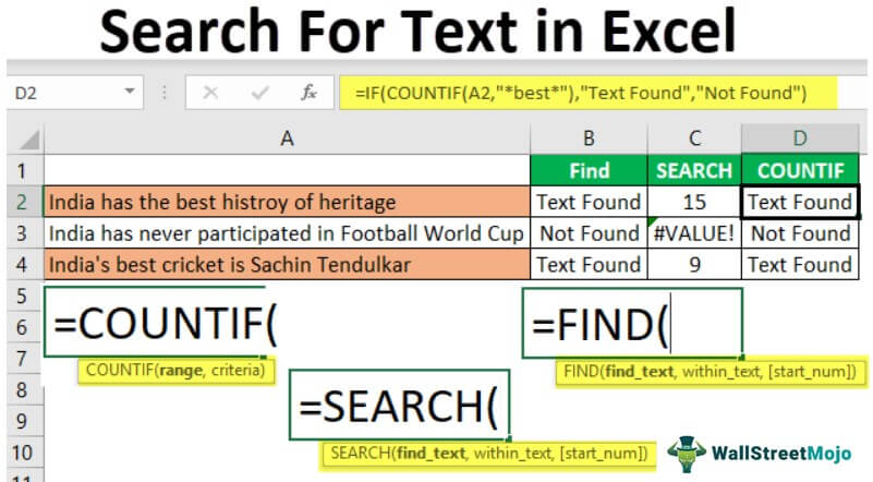
It is a question we have seen many times in Excel forums. The first formula that came to mind was the “FIND” function.
The FIND function can return the position of the supplied text values in the string. So, if the FIND method returns any number, then we can consider the cell as it has the text or else not.
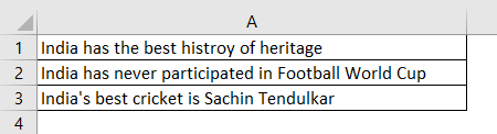
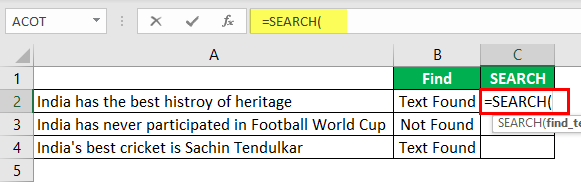
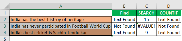
- For example, look at the below data.

- In the above data, we have three sentences in three different rows. Now in each cell, we need to search for the text “Best.” So, apply the FIND function.

- The “find_text” argument mentions the text we need to find.

- For the “within_text,” select the full sentence, i.e., cell reference.

- The last parameter is not required to close the bracket and press the “Enter” key.

So, in two sentences, we have the word “best.” We can see the error value of #VALUE! in cell B2, which shows that cell A2 does not have the text value “best.”
- Instead of numbers, we can also enter the result in our own words. For this, we need to use the IF condition.


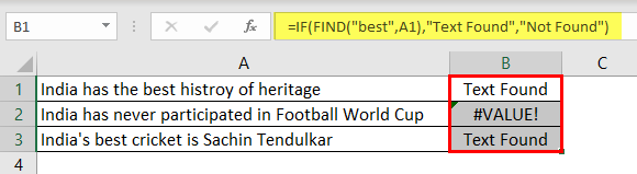
So, in the IF condition, we have supplied the result as “Text Found” if the value “best” is found. Otherwise, we have provided the result as “Not Found.”
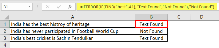
But, here we have a problem, even though we have supplied the result as “Not Found,” if the text is still not found, we are getting the error value as #VALUE!.
So, nobody wants to have an error value in their Excel sheet. Therefore, we must enclose the formula with the ISNUMERIC function to overcome this error value.

The ISNUMERIC function evaluates whether the FIND function returns the number or not. If the FIND function returns the number, it will supply TRUE to the IF condition or else FALSE condition. Based on the result provided by the ISNUMERIC function, the IF condition will return the result accordingly.
We can also use the IFERROR function in excelThe IFERROR function in Excel checks a formula (or a cell) for errors and returns a specified value in place of the error.read more to deal with error values instead of ISNUMERIC. For example, the below formula will also return “Not Found” if the FIND function returns the error value.
Alternatives to FIND Function
Alternative #1 – Excel Search Function
Instead of the FIND function, we can also use the SEARCH function in excelSearch function gives the position of a substring in a given string when we give a parameter of the position to search from. As a result, this formula requires three arguments. The first is the substring, the second is the string itself, and the last is the position to start the search.read more to search the particular text in the string. The syntax of the SEARCH function is the same as the FIND function.
Supply the “find_text” as “Best.”
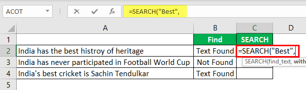
The “within_text” is our cell reference.
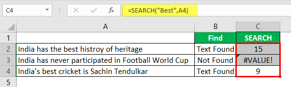
Even the SEARCH function returns an error value as #VALUE! If the finding text “best” is not found. As we have seen above, we need to enclose the formula with ISNUMERIC or IFERROR functions.
Alternative #2 – Excel Countif Function
Another way to search for a particular text is using the COUNTIF functionThe COUNTIF function in Excel counts the number of cells within a range based on pre-defined criteria. It is used to count cells that include dates, numbers, or text. For example, COUNTIF(A1:A10,”Trump”) will count the number of cells within the range A1:A10 that contain the text “Trump”
read more. This function works without any error.
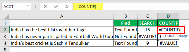
In the range, the argument selects the cell reference.
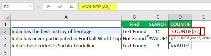
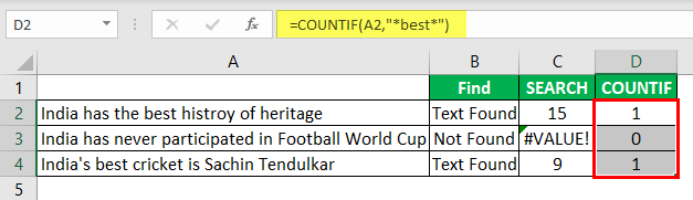
In the criteria column, we need to use a wildcard in excelIn Excel, wildcards are the three special characters asterisk, question mark, and tilde. Asterisk denotes multiple characters, a question mark denotes a single character, and a tilde denotes the identification of a wild card character.read more because we are just finding the part of the string value, so enclose the word “best” with an asterisk (*) wildcard.
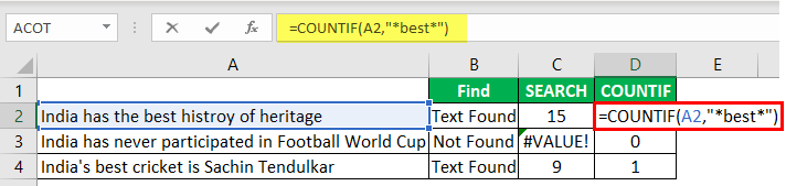
This formula will return the word “best” count in the selected cell value. Since we have only one “best” value, we will get only 1 as the count.
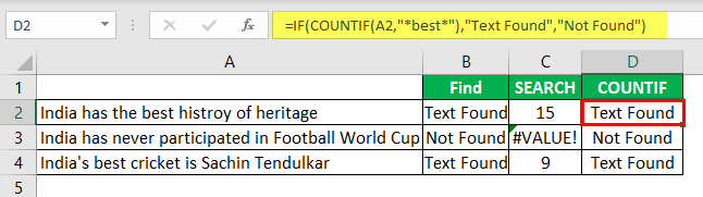
We can apply only the IF condition to get the result without error.
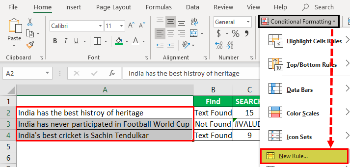
Highlight the Cell which has a Particular Text Value
If you are not a fan of formulas, you can highlight the cell with a particular word. For example, to highlight the cell with the word “best,” we need to use conditional formatting in excelConditional formatting is a technique in Excel that allows us to format cells in a worksheet based on certain conditions. It can be found in the styles section of the Home tab.read more.
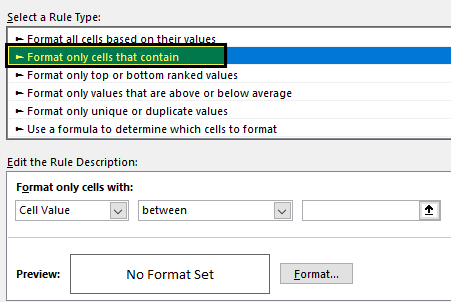
First, select the data cells and click “Conditional Formatting” > “New Rule.”
Under “New Rule,” select the “Format only cells that contain” option.
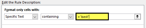
From the first dropdown, select “Specific Text.”

The formula section enters the text we search for in double quotes with the equal sign. =’best.’
Then, click on “FORMAT” and choose the formatting style.
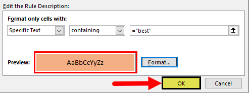
Click on “OK.” It will highlight all the cells which have the word “best.”
Using various techniques, we can search the particular text in Excel.
Recommended Articles
This article is a guide to Search For Text in Excel. Here, we discuss the top three methods to search the cell value for a specific text and arrive at the result with practical examples and a downloadable Excel template. You may learn more about Excel from the following articles: –
- Find Links in Excel
- Using Find and Select in Excel
- Search Box in Excel