
Excel for Microsoft 365 Excel for Microsoft 365 for Mac Excel 2021 Excel 2021 for Mac Excel 2019 Excel 2019 for Mac Excel 2016 Excel 2016 for Mac Excel 2013 Excel 2010 Excel 2007 More…Less
This topic provides help for the most common scenarios for the #VALUE! error in the FIND/FINDB and SEARCH/SEARCHB functions.
A few things to know about FIND and SEARCH functions
-
The FIND and SEARCH functions are very similar. They both work in the same way — locate a character or a text string in another text string. The difference between these two functions is that FIND is case-sensitive, and SEARCH is not case-sensitive. So if you don’t want to match case in a text string, use SEARCH.
-
If you want a function that returns the string based on the character number you specify, use the MID function along with FIND. You can find information and examples of using MID and FIND combinations in the FIND help topic.
-
The syntax of these functions is the same, find_text, within_text, [start_num]). In simple English, the syntax means What do you want to find?, Where do you want to find it?, What position do you want to start from?
Problem: the value in the find_text argument cannot be found in the within_text string
If the function cannot find the text to be found in the specified text string, it will throw a #VALUE! error.
For example, a function like:
-
=FIND(«gloves»,»Gloves (Youth)»,1)
Will throw the #VALUE! error, because there is no matching “gloves” in the string, but there is “Gloves”. Remember that FIND is case-sensitive, so make sure the value in find_text has an exact match in the string in the within_text argument.
However, this SEARCH function will return a value of 1, since it’s not case-sensitive:
-
=SEARCH(«gloves»,»Gloves (Youth)»,1)
Solution: Correct the syntax as necessary.
Problem: The start_num argument is set to zero (0)
The start_num argument is an optional argument, and if you omit it, the default value will be assumed to be 1. However, if the argument is present in the syntax and the value is set to 0, you will see the #VALUE! error.
Solution: Remove the start_num argument if it is not required, or set it to the correct appropriate value.
Problem: The start_num argument is greater than the within_text argument
For example, the function:
-
=FIND(“s”,”Functions and formulas”,25)
Looks for “s” in the “Functions and formulas” string (within_text) starting at the 25th character (start_num), but returns a #VALUE! error because there are only 22 characters in the string.
Tip: To find the total number of characters in a text string, use the LEN function
Solution: Correct the starting number as necessary.
Need more help?
You can always ask an expert in the Excel Tech Community or get support in the Answers community.
See Also
Correct a #VALUE! error
FIND/FINDB functions
SEARCH/SEARCHB FUNCTIONS
Overview of formulas in Excel
How to avoid broken formulas
Detect errors in formulas
All Excel functions (alphabetical)
All Excel functions (by category)
Need more help?
Want more options?
Explore subscription benefits, browse training courses, learn how to secure your device, and more.
Communities help you ask and answer questions, give feedback, and hear from experts with rich knowledge.
This is an old question but a solution for those using Excel 2016 or newer is you can remove the need for nested if structures by using the new IFS( condition1, return1 [,condition2, return2] ...) conditional.
I have formatted it to make it visually clearer on how to use it for the case of this question:
=IFS(
ISERROR(SEARCH("String1",A1))=FALSE,"Something1",
ISERROR(SEARCH("String2",A1))=FALSE,"Something2",
ISERROR(SEARCH("String3",A1))=FALSE,"Something3"
)
Since SEARCH returns an error if a string is not found I wrapped it with an ISERROR(...)=FALSE to check for truth and then return the value wanted. It would be great if SEARCH returned 0 instead of an error for readability, but thats just how it works unfortunately.
Another note of importance is that IFS will return the match that it finds first and thus ordering is important. For example if my strings were Surf, Surfing, Surfs as String1,String2,String3 above and my cells string was Surfing it would match on the first term instead of the second because of the substring being Surf. Thus common denominators need to be last in the list. My IFS would need to be ordered Surfing, Surfs, Surf to work correctly (swapping Surfing and Surfs would also work in this simple example), but Surf would need to be last.
invirtus

Пользователь
Сообщений: 33
Регистрация: 27.03.2015
Добрый день всем.
Возникла проблема с методом Find. Вчера убил два часа, но так и не понял, почему он то работает, то нет. Через Find и Offset я пытаюсь сэмулировать экселевский Vlookup. Есть исходный файл с двумя колонками — в первой список ИНН, во второй — список номеров поставщиков. Макрос в testFile находит ИНН (с этим он прекрасно справляется), а потом используя ИНН должен искать мне номер поставщика. Он то работал вчера, то нет. Когда не работал, я сохранял файл, закрывал, открывал, запускал макрос построчно и по коду следил, что происходит после выполнения каждой строки, и он находил поставщика. Потом закрывал файл, открывал, запускал просто так и он не находил поставщика. Выкладываю файл где ищется ИНН и файл со списком поставщиков (готовый макрос не влезает по максимальному объему файла). Необходимый макрос — Sub PriceListShow(). Ниже интересующий меня блок кода, я не пойму, почему он не работает (уже перебрал все возможные варианты, но он так и не ищет строку).
Я начал грешить на то, что у меня String, а в файле со списком поставщиков формат данных «цифровой», но смена переменной на Double никакого результата не принесла.
Как видите ниже, я перепробовал различные варианты запросов (даже vlookup), но опять таки к какому то очевидному пониманию не пришёл. Надеюсь вы мне поможете и/или подскажете, как улучшить код.
Спасибо.
| Код |
|---|
On Error Resume Next
Dim SupplierINN As String
Dim SupplierBlockStart As String
Dim SupplierBlockEnd As String
SupplierBlockStart = Worksheets("Данные поставщика").Range("A1:C100").Find("*Контак*ормация*поставщика*").Address
SupplierBlockEnd = Worksheets("Данные поставщика").Range("A1:C100").Find("лицо*поставщика*").Address
SupplierINN = Worksheets("Данные поставщика").Range(Worksheets("Данные поставщика").Range(SupplierBlockStart & ":" & SupplierBlockEnd).Find("*ИНН*").Address).Offset(, 1).Value

If SupplierINN = Empty Then
PriceListAuto.Supplier = "НЕТ ИНН"
PriceListAuto.Supplier.BackColor = RGB(254, 230, 61)
PriceListAuto.SupplierLabel = "На вкладке ""Данные поставщика"" не указан ИНН. Уточните ИНН / Введите вручную"
Else

'xSupplier = Workbooks("PrismaTools.xlsm").Worksheets("Suppliers").Range(Range("A:A").Find(SupplierINN, , , xlPart).Address).Offset(, 2).Value
'If xSupplier = "" Then xSupplier = Workbooks("PrismaTools.xlsm").Worksheets("Suppliers").Range(Range("A:A").Find(SupplierINN, , , xlWhole).Address).Offset(, 2).Value
'If xSupplier = "" Then xSupplier = Workbooks("PrismaTools.xlsm").Worksheets("Suppliers").Range(Range("A:A").Find("*" & SupplierINN & "*", , , xlPart).Address).Offset(, 2).Value
'If xSupplier = "" Then xSupplier = Workbooks("PrismaTools.xlsm").Worksheets("Suppliers").Range(Range("A:A").Find("*" & SupplierINN & "*", , , xlWhole).Address).Offset(, 2).Value
If xSupplier = "" Then xSupplier = Workbooks("PrismaTools.xlsm").Worksheets("Suppliers").Application.WorksheetFunction.VLookup(CDbl(SupplierINN), "A:C", 3, 0)

xSupplierName = Workbooks("Suppliers.xlsm").Worksheets("Suppliers").Range(Range("C:C").Find(xSupplier, , , xlPart).Address).Offset(, 1).Value
If xSupplier = "" Then
PriceListAuto.Supplier = "НЕ НАЙДЕН"
PriceListAuto.SupplierLabel = "Поставщик не найден. Проверьте список поставщиков или введите номер вручную"
Else
PriceListAuto.Supplier = xSupplier
PriceListAuto.Supplier.BackColor = RGB(107, 198, 6)
PriceListAuto.SupplierLabel = xSupplierName
End If
End If
|
Изменено: invirtus — 28.07.2015 10:03:13
![]()
Excel If Cell Contains Text

Excel If Cell Contains Text Then Formula helps you to return the output when a cell have any text or a specific text. You can check if a cell contains a some string or text and produce something in other cell. For Example you can check if a cell A1 contains text ‘example text’ and print Yes or No in Cell B1. Following are the example Formulas to check if Cell contains text then return some thing in a Cell.
If Cell Contains Text
Here are the Excel formulas to check if Cell contains specific text then return something. This will return if there is any string or any text in given Cell. We can use this simple approach to check if a cell contains text, specific text, string, any text using Excel If formula. We can use equals to operator(=) to compare the strings .
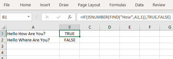
If Cell Contains Text Then TRUE
Following is the Excel formula to return True if a Cell contains Specif Text. You can check a cell if there is given string in the Cell and return True or False.
The formula will return true if it found the match, returns False of no match found.
If Cell Contains Partial Text
We can return Text If Cell Contains Partial Text. We use formula or VBA to Check Partial Text in a Cell.
Find for Case Sensitive Match:
We can check if a Cell Contains Partial Text then return something using Excel Formula. Following is a simple example to find the partial text in a given Cell. We can use if your want to make the criteria case sensitive.
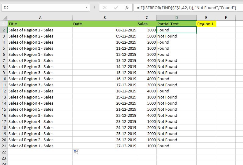
- Here, Find Function returns the finding position of the given string
- Use Find function is Case Sensitive
- IsError Function check if Find Function returns Error, that means, string not found
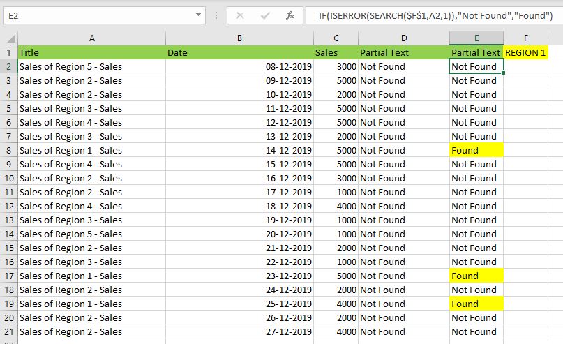
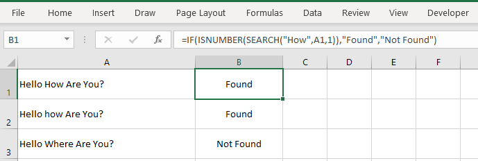
Search for Not Case Sensitive Match:
We can use Search function to check if Cell Contains Partial Text. Search function useful if you want to make the checking criteria Not Case Sensitive.
If Range of Cells Contains Text
We can check for the strings in a range of cells. Here is the formula to find If Range of Cells Contains Text. We can use Count If Formula to check the excel if range of cells contains specific text and return Text.
- CountIf function counts the number of cells with given criteria
- We can use If function to return the required Text
- Formula displays the Text ‘Range Contains Text” if match found
- Returns “Text Not Found in the Given Range” if match not found in the specified range
If Cells Contains Text From List
Below formulas returns text If Cells Contains Text from given List. You can use based on your requirement.
VlookUp to Check If Cell Contains Text from a List:
We can use VlookUp function to match the text in the Given list of Cells. And return the corresponding values.
- Check if a List Contains Text:
=IF(ISERR(VLOOKUP(F1,A1:B21,2,FALSE)),”False:Not Contains”,”True: Text Found”) - Check if a List Contains Text and Return Corresponding Value:
=VLOOKUP(F1,A1:B21,2,FALSE) - Check if a List Contains Partial Text and Return its Value:
=VLOOKUP(“*”&F1&”*”,A1:B21,2,FALSE)
If Cell Contains Text Then Return a Value
We can return some value if cell contains some string. Here is the the the Excel formula to return a value if a Cell contains Text. You can check a cell if there is given string in the Cell and return some string or value in another column.
The formula will return true if it found the match, returns False of no match found. can
Excel if cell contains word then assign value
You can replace any word in the following formula to check if cell contains word then assign value.
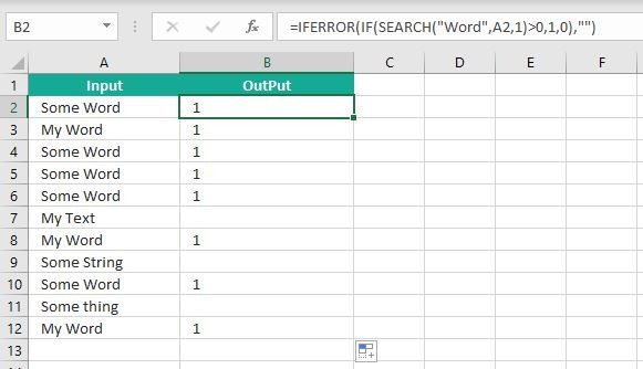
Search function will check for a given word in the required cell and return it’s position. We can use If function to check if the value is greater than 0 and assign a given value (example: 1) in the cell. search function returns #Value if there is no match found in the cell, we can handle this using IFERROR function.
Count If Cell Contains Text
We can check If Cell Contains Text Then COUNT. Here is the Excel formula to Count if a Cell contains Text. You can count the number of cells containing specific text.
The formula will Sum the values in Column B if the cells of Column A contains the given text.
Count If Cell Contains Partial Text
We can count the cells based on partial match criteria. The following Excel formula Counts if a Cell contains Partial Text.
- We can use the CountIf Function to Count the Cells if they contains given String
- Wild-card operators helps to make the CountIf to check for the Partial String
- Put Your Text between two asterisk symbols (*YourText*) to make the criteria to find any where in the given Cell
- Add Asterisk symbol at end of your text (YourText*) to make the criteria to find your text beginning of given Cell
- Place Asterisk symbol at beginning of your text (*YourText) to make the criteria to find your text end of given Cell
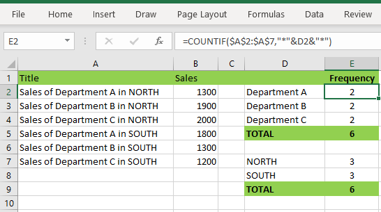
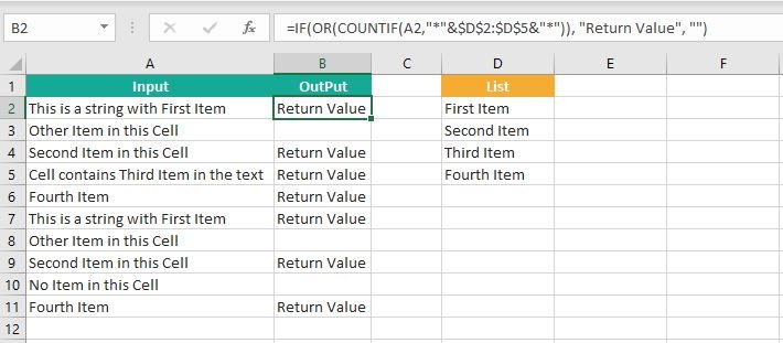
If Cell contains text from list then return value
Here is the Excel Formula to check if cell contains text from list then return value. We can use COUNTIF and OR function to check the array of values in a Cell and return the given Value. Here is the formula to check the list in range D2:D5 and check in Cell A2 and return value in B2.
If Cell Contains Text Then SUM
Following is the Excel formula to Sum if a Cell contains Text. You can total the cell values if there is given string in the Cell. Here is the example to sum the column B values based on the values in another Column.
The formula will Sum the values in Column B if the cells of Column A contains the given text.

Sum If Cell Contains Partial Text
Use SumIfs function to Sum the cells based on partial match criteria. The following Excel formula Sums the Values if a Cell contains Partial Text.
- SUMIFS Function will Sum the Given Sum Range
- We can specify the Criteria Range, and wild-card expression to check for the Partial text
- Put Your Text between two asterisk symbols (*YourText*) to Sum the Cells if the criteria to find any where in the given Cell
- Add Asterisk symbol at end of your text (YourText*) to Sum the Cells if the criteria to find your text beginning of given Cell
- Place Asterisk symbol at beginning of your text (*YourText) to Sum the Cells if criteria to find your text end of given Cell
VBA to check if Cell Contains Text
Here is the VBA function to find If Cells Contains Text using Excel VBA Macros.
If Cell Contains Partial Text VBA
We can use VBA to check if Cell Contains Text and Return Value. Here is the simple VBA code match the partial text. Excel VBA if Cell contains partial text macros helps you to use in your procedures and functions.
MsgBox CheckIfCellContainsPartialText(Cells(2, 1), “Region 1”)
End Sub
Function CheckIfCellContainsPartialText(ByVal cell As Range, ByVal strText As String) As Boolean
If InStr(1, cell.Value, strText) > 0 Then CheckIfCellContainsPartialText = True
End Function
- CheckIfCellContainsPartialText VBA Function returns true if Cell Contains Partial Text
- inStr Function will return the Match Position in the given string
If Cell Contains Text Then VBA MsgBox
Here is the simple VBA code to display message box if cell contains text. We can use inStr Function to search for the given string. And show the required message to the user.
If InStr(1, Cells(2, 1), “Region 3”) > 0 Then blnMatch = True
If blnMatch = True Then MsgBox “Cell Contains Text”
End Sub
- inStr Function will return the Match Position in the given string
- blnMatch is the Boolean variable becomes True when match string
- You can display the message to the user if a Range Contains Text
Which function returns true if cell a1 contains text?
You can use the Excel If function and Find function to return TRUE if Cell A1 Contains Text. Here is the formula to return True.
Which function returns true if cell a1 contains text value?
You can use the Excel If function with Find function to return TRUE if a Cell A1 Contains Text Value. Below is the formula to return True based on the text value.
Share This Story, Choose Your Platform!
7 Comments
-
Meghana
December 27, 2019 at 1:42 pm — ReplyHi Sir,Thank you for the great explanation, covers everything and helps use create formulas if cell contains text values.
Many thanks! Meghana!!
-
Max
December 27, 2019 at 4:44 pm — ReplyPerfect! Very Simple and Clear explanation. Thanks!!
-
Mike Song
August 29, 2022 at 2:45 pm — ReplyI tried this exact formula and it did not work.
-
Theresa A Harding
October 18, 2022 at 9:51 pm — Reply -
Marko
November 3, 2022 at 9:21 pm — ReplyHi
Is possible to sum all WA11?
(A1) WA11 4
(A2) AdBlue 1, WA11 223
(A3) AdBlue 3, WA11 32, shift 4
… and everything is in one column.
Thanks you very much for your help.
Sincerely Marko
-
Mike
December 9, 2022 at 9:59 pm — ReplyThank you for the help. The formula =OR(COUNTIF(M40,”*”&Vendors&”*”)) will give “TRUE” when some part of M40 contains a vendor from “Vendors” list. But how do I get Excel to tell which vendor it found in the M40 cell?
-
PNRao
December 18, 2022 at 6:05 am — ReplyPlease describe your question more elaborately.
Thanks!
-
© Copyright 2012 – 2020 | Excelx.com | All Rights Reserved
Page load link
This post will guide you how to use Excel FIND function with syntax and examples in Microsoft excel.
Table of Contents
- Description
- Syntax
- Excel Find Function Examples
- Frequently Asked Questions
- Related Functions
- More FIND Formula Examples in Excel
Description
The Excel FIND function returns the position of the first text string (sub string) within another text string.
It can be used when you want to get the position of a sub string inside another text string. so it will return a number that indicates the starting position of sub string that you are searching in another text string.
The FIND function is a build-in function in Microsoft Excel and it is categorized as a Text Function.
Note: The FIND Function is case-sensitive.
The FIND function is available in Excel 2016, Excel 2013, Excel 2010, Excel 2007, Excel 2003, Excel xp, Excel 2000, Excel 2011 for Mac.
Syntax
The syntax of the FIND function is as below:
= FIND(find_text, within_text,[start_num])
Where the FIND function arguments are:
- Find_text -This is a required argument. The text or substring that you want to find. (The string in the Find_text argument can not contain any wildcard characters)
- within_text -This is a required argument. The text string that is to be searched
- start_num-This is an optional argument. It will specify the position in within text string where the search will start. If you omit start_num value, the search will start from the first character of the within_text string, in other words, it is set to be 1 by default. So you can use the Excel Find function to look for the specified text starting from the specified position.
Note:
- The Find function will return the position of the first character of find_text in within_text argument.
- If there are several occurrences of the find_text within another text string, it only return the position of the first occurrence.
- If the find_text is an empty string, the position of the first character in the within_text is returned.
- If the find_text string is not found in within_text, it will return the Excel #VALUE! Error.
- If start_number value is not greater than 0, it will return the #VALUE! Error value.
- As the FIND function is case-sensitive. If you want to do a search that is case-insensitive , you can use the SEARCH Function.
- The FIND function does not support wildcard characters, so if you want to use wildcard characters to find string, you can use SEARCH function in excel.
Excel Find Function Examples
The below example will show you how to use Excel FIND Text function to find the position of a sub string within text string.
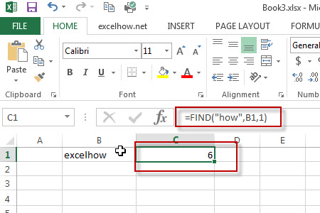
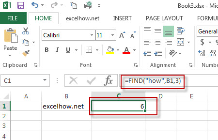
#1 To get the position of sub string “how” in cell B1, just using formula:
=FIND("how",B1,1).
When you look for the text “how” in the Cell B1, it will return 6, which is the position of the first character of find_text “how” within the Cell B1.
#2 To get the position of sub string “how”in cell b1, starting with the third character, using formula:
=FIND("how",B1,3)
In the above example, it specified the start_num value as “3“, so you will get the position of the first character “h” of the searched string “how” within the value in Cell B1 when the starting position is 3. it returns 6.
The Example 1The search will start from the third character of the value in Cell B1.
#3 Finding “excel” string in Cell B1, using the following Find formula:
=FIND("excel",B1,1)
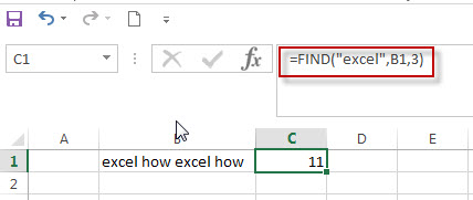
=FIND("excel",B1,3)
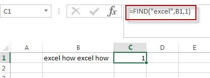
when you set the starting position as 1, it will return the position of the first “excel” string in the value of Cell B1.
When you set the starting position as 3, it will return the position of the second “excel” string in the value of Cell B1. The search will start from the third character of the value in Cell B1.
#4 Searching an empty string in Cell B1, using the following Find formula:
=FIND("",B1,1)
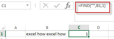
In the above example, when you look for an empty string in Cell B1 with the starting position as 1, and it will return the position of the first character of the within_ text (the value of Cell B1).
#5 Searching “word” text in Cell B1, using the following Find formula:
=FIND("word", B1,1)
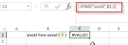
In the above example, when you look for the text “word” in Cell B1 and the string position is 1, it will return a #VALUE! error, As the searched string “word” is not found in Cell B1.
#6 Searching for a text as “excel” in Cell B1 and the starting position is a negative number.
=FIND("excel",B1,-1)
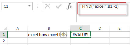
If the starting position is not greater than 0, it will return a #VALUE! Error.
#7 Searching for a string as “EXCEL” in Cell B1, using the following formula:
=FIND("EXCEL",B1,1)
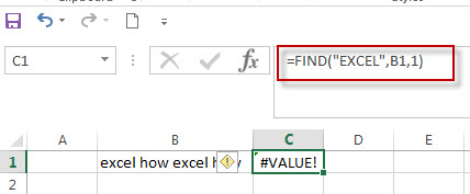
As the FIND function in excel is case-sensitive, when you look for the string “EXCEL” in Cell B1, the searched string “EXCEL” is not found, the function will return a #VALUE! error.
Frequently Asked Questions
Question 1: the FIND function returns a #VALUE error when it do not find the searched text within another string. I want to know if there is another excel function in combination with the find function to handle the error message to return the actual value, such as: -1 or throwing others exceptions via returning values, like: -1,0 or FALSE.
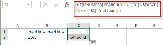
Answer: As mentioned above, the FIND function is case-sensitive, and it can be combined with the ISNUMBER function and IF function to create a new IF excel formula as follows:
=IF(ISNUMBER( FIND("excel",B1)), FIND("excel",B1), "not found")
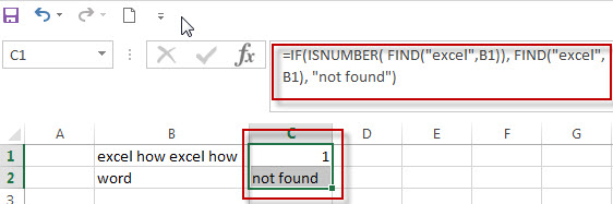
The FIND function will locate the position of the searched text “excel” within Cell B1, and the ISNUMBER function will check the result returned by the FIND function if it is a number, if TRUE, then return TRUE, otherwise , returns FALSE. then the IF will check the Boolean value returned by ISNUMBER function, If TRUE, then returns the numeric position returned by the second FIND function, If FALSE, returns “not found” string.
If you want a case-insensitive match and you can use the SEARCH function instead of the FIND function in the above formula:
=IF(ISNUMBER( SEARCH("excel",B1)), SEARCH("excel",B1), "not found")
Question 2: I want to extract a sub string from a string that separated by wildcard characters. I tried to use the below FIND formula to handle it. but it returned a #VALUE error message. Could you please help to check the below formula I used:
=RIGHT(B1,FIND("~**",B1))
Answer: you can use the following formula:
=TRIM(RIGHT(B1,Len(B1) - FIND("**",B1)-1))
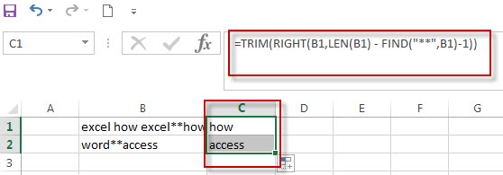
The find function will return the position of the first wildcard (**) character within a string in Cell B1. you need subtract the numeric position returned by FIND function from the length of the string in Cell B1 to get the length of sub string to the right of the wildcard character(asterisk). then the RIGHT function extracts the rightmost characters based on the length of sub string.
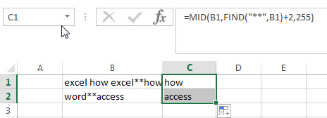
or you can use another formula to achieve the same result as follows:
=MID(B1,FIND("**",B1)+2,255)
Question 3: I am trying to extract the first word from another text string separated by space character. but it always return a #VALUE error message. I think it should be use the FIND function in combination with another function, such as: left function. but I still don’t know how to combine with those two functions to extract the first word.
Answer: right, you can create a excel formula that uses the FIND function and LEFT function. and you can use the below formula:
=IFERROR(LEFT(B1, FIND(" ",B1)-1),B1)
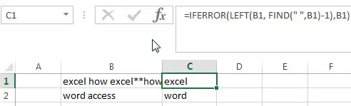
The find function returns the position of the first space character in the text string in Cell B1. the Formula “=FIND(” “,B1)-1 returns the numbers of the first word as the second arguments of the LEFT function.
If the text string in Cell B1 just only contains one word, then the find function will return #VALUE error. to handle this error, you need to use the IFERROR function, if the find function is not find the space character, then return the text string in B1. in other words, it just contains only one word in Cell B1.
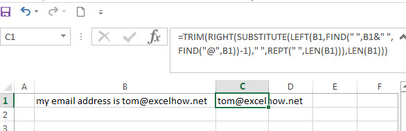
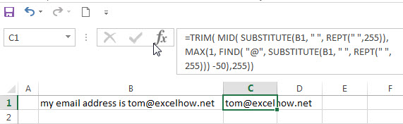
Question 4: I am trying to extract an email address from a text string in Cell B1. how to write a excel formula to achieve the result.
Answer: you can use a combination of the TRIM function, the LEFT function, the SUBSTITUTE function, the MID function, the MAX function and the REPT function to create a complex excel formula to extract email address from a string in Cell B1.
=TRIM(RIGHT(SUBSTITUTE(LEFT(B1,FIND (" ",B1&" ",FIND("@",B1))-1)," ", REPT(" ",LEN(B1))),LEN(B1)))
=TRIM( MID( SUBSTITUTE(B1, " ", REPT(" ",255)), MAX(1, FIND( "@", SUBSTITUTE(B1, " ", REPT(" ",255))) -50),255))
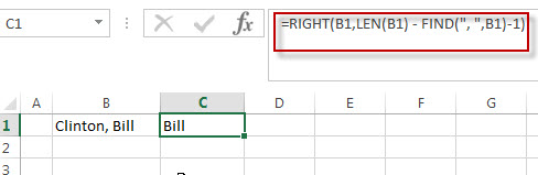
Question 5: I am trying to get the first name from a full name separated by a comma character. how to use a excel formula to extract the first name from a name as: “Last name, First name” format.
Answer: you can use a combination with the RIGHT function, the LEN function and the FIND function to create a excel formula to get the first name from a name. just using the following formula:
=RIGHT(B1,LEN(B1) - FIND(", ",B1)-1)
- Excel SEARCH function
The Excel SEARCH function returns the number of the starting location of a substring in a text string.The syntax of the SEARCH function is as below:= SEARCH (find_text, within_text,[start_num])… - Excel Find function
The Excel FIND function returns the position of the first text string (substring) from the first character of the second text string.The FIND function is a build-in function in Microsoft Excel and it is categorized as a Text Function.The syntax of the FIND function is as below:= FIND (find_text, within_text,[start_num])… - Excel ISERROR function
The Excel ISERROR function returns TRUE if the value is any error value except #N/A. The ISERROR function is a build-in function in Microsoft Excel and it is categorized as an Information Function. The syntax of the ISERROR function is as below: = ISERROR (value) … - Excel ISNUMBER function
The Excel ISNUMBER function returns TRUE if the value in a cell is a numeric value, otherwise it will return FALSE.The syntax of the ISNUMBER function is as below:= ISNUMBER (value)… - Excel RIGHT function
The Excel RIGHT function returns a sub string (a specified number of the characters) from a text string, starting from the rightmost character.The syntax of the RIGHT function is as below:= RIGHT (text,[num_chars])… - Excel LEN function
The Excel LEN function returns the length of a text string (the number of characters in a text string).The LEN function is a build-in function in Microsoft Excel and it is categorized as a Text Function.The syntax of the LEN function is as below:= LEN(text)… - Excel MID function
The Excel MID function returns a sub string from a text string at the position that you specify. The MID function is a build-in function in Microsoft Excel and it is categorized as a Text Function. The syntax of the MID function is as below: = MID (text, start_num, num_chars) … - Excel SUBSTITUTE function
The Excel SUBSTITUTE function replaces a new text string for an old text string in a text string.The syntax of the SUBSTITUTE function is as below:= SUBSTITUTE (text, old_text, new_text,[instance_num])… - Excel LEFT function
The Excel LEFT function returns a sub string (a specified number of the characters) from a text string, starting from the leftmost character.The LEFT function is a build-in function in Microsoft Excel and it is categorized as a Text Function.The syntax of the LEFT function is as below:= LEFT(text,[num_chars])… - Excel REPT function
The Excel REPT function repeats a text string a specified number of times.The REPT function is a build-in function in Microsoft Excel and it is categorized as a Text Function.The syntax of the REPT function is as below:= REPT (text, number_times)…
More FIND Formula Examples in Excel
-
Split Text String by Specified Character
you should use the Left function in combination with FIND function to split the text string in excel. And we can refer to the below formula that will find the position of “-“in Cell B1 and extract all the characters to the left of the dash character “-“.=LEFT(B1,FIND(“-“,B1,1)-1).… - Split Text String by Line Break
When you want to split text string by line break in excel, you should use a combination of the LEFT, RIGHT, CHAR, LEN and FIND functions. The CHAR (10) function will return the line break character, the FIND function will use the returned value of the CHAR function as the first argument to locate the position of the line break character within the cell B1.… - Split Text and Numbers in Excel
If you want to split text and numbers, you can run the following excel formula that use the MIN function, FIND function and the LEN function within the LEFT function in excel. .… - Get the Current Worksheet Name only
If you want to get the current worksheet name only in excel, you can use a combination of the MID function, the CELL function and FIND function.… - Get full File Name (workbook and worksheet) and Path
In excel, you can get the current workbook name and it is absolute path using the CELL function. Just refer to the following formula:=CELL(“filename”,B1).… - Get the Current Workbook Name
If you want to get the name of the current workbook only, you can use a combination of the MID function, the CELL function and the FIND Function… - Get Path and Workbook name only
If you want to get the workbook name and its path only without worksheet name, you can use a combination of the SUBSTITUTE function, the LEFT function, the CELL function and the FIND function…. - Get First Name From Full Name
If you want to get the first name from a full name list in Column B, you can use the FIND function within LEFT function in excel. The generic formula is as follows:=LEFT(B1,FIND(” “,B1)-1).… - Get Last Name From Full Name
To extract the last name within a Full name in excel. You need to use a combination of the RIGHT function, the LEN function, the FIND function and the SUBSTITUTE function to create a complex formula in excel..… - The different between FIND and SEARCH functions
There are two big differences between FIND and SEARCH functions in excel.The FIND function is case-sensitive. And the SEARCH function is case-insensitive…… - Data Validation for Specified Text only
If you want to check if the values that contain a specified text string in one cell, you can use a combination of the FIND function and ISNUMBER function as a formula in the Data Validation….… - Count Cells That Contain Specific Text
This post will discuss that how to count the number of cells that contain specific text or certain text in a specified cells of range in Excel. How to get the total number of cells that contain certain text.…… - Split Text and Numbers
If you want to split text and numbers from one cell into two different cells, you can use a formula based on the FIND function, the LEFT function or the RIGHT function and the MIN function. .… - Quickly Get Sheet Name
If you want to quickly get current worksheet name only, then inert it into one cell. You can use a formula based on the MID function in combination with the FIND function and the Cell function…… - Sorting IP Address
Assuming that you have an IP list of data in the range of cells B1:B5, and you want to sort those IP list from low to high, how to achieve the result with excel formula. You need to create a formula based on the Text Function, the LEFT function, the FIND function and the MID function, the RIGHT function..… - Removing Salutation from Name
To remove salutation from names string in excel, you can create a formula based on the RIGHT function, the LEN function and the FIND function…… - List all Worksheet Names
Assuming that you have a workbook that has hundreds of worksheets and you want to get a list of all the worksheet names in the current workbook. And the below will introduce 3 methods with you..… - Insert The File Path and Filename into Cell
If you want to insert a file path and filename into a cell in your current worksheet, you can use the CELL function to create a formual……..