
Purpose
Get location substring in a string
Return value
A number representing the location of substring
Usage notes
The FIND function returns the position (as a number) of one text string inside another. If there is more than one occurrence of the search string, FIND returns the position of the first occurrence. When the text is not found, FIND returns a #VALUE error. Also note, when find_text is empty, FIND returns 1. FIND does not support wildcards, and is always case-sensitive. Use the SEARCH function to find the position of text without case-sensitivity and with wildcard support.
Basic Example
The FIND function is designed to look inside a text string for a specific substring. When FIND locates the substring, it returns a position of the substring in the text as a number. If the substring is not found, FIND returns a #VALUE error. For example:
=FIND("p","apple") // returns 2
=FIND("z","apple") // returns #VALUE!
Note that text values entered directly into FIND must be enclosed in double-quotes («»).
Case-sensitive
The FIND function always case-sensitive:
=FIND("a","Apple") // returns #VALUE!
=FIND("A","Apple") // returns 1
TRUE or FALSE result
To force a TRUE or FALSE result, nest the FIND function inside the ISNUMBER function. ISNUMBER returns TRUE for numeric values and FALSE for anything else. If FIND locates the substring, it returns the position as a number, and ISNUMBER returns TRUE:
=ISNUMBER(FIND("p","apple")) // returns TRUE
=ISNUMBER(FIND("z","apple")) // returns FALSE
If FIND doesn’t locate the substring, it returns an error, and ISNUMBER returns FALSE.
Start number
The FIND function has an optional argument called start_num, that controls where FIND should begin looking for a substring. To find the first match of «the» in any combination of upper or lowercase, you can omit start_num, which defaults to 1:
=FIND("x","20 x 30 x 50") // returns 4To start searching at character 5, enter 4 for start_num:
=FIND("x","20 x 30 x 50",5) // returns 9
Wildcards
The FIND function does not support wildcards. See the SEARCH function.
If cell contains
To return a custom result with the SEARCH function, use the IF function like this:
=IF(ISNUMBER(FIND(substring,A1)), "Yes", "No")
Instead of returning TRUE or FALSE, the formula above will return «Yes» if substring is found and «No» if not.
Notes
- The FIND function returns the location of the first find_text in within_text.
- The location is returned as the number of characters from the start.
- Start_num is optional and defaults to 1.
- FIND returns 1 when find_text is empty.
- FIND returns #VALUE if find_text is not found.
- FIND is case-sensitive but does not support wildcards.
- Use the SEARCH function to find a substring with wildcards.
I have the formula:
=LOOKUP(C2,'Jul-14'!A:A,'Jul-14'!B:B)
Where:
C2= «Aruba (AW)»
The sheet «Jul-14» doesn’t contain the value «Aruba (AW)» in column A. When this happens, it seems to take the closet match and return the value in column B. I need it to return 0 if no exact match is found, or the B column value if an exact match is found.
I’ve tried changing the function to VLOOKUP and HLOOKUP but it doesn’t ever return any value.
asked Apr 13, 2015 at 10:55
![]()
Tom GullenTom Gullen
60.7k83 gold badges280 silver badges454 bronze badges
1
The following should lookup the value in C2 against the values on the sheet in column A, if it finds a match then it will show it, if it doesn’t then it will throw an error which will then return 0
=iferror(vlookup(C2,'Jul-14'!A:B,2,False),0)
answered Apr 13, 2015 at 11:05
![]()
Excel for Microsoft 365 Excel for Microsoft 365 for Mac Excel for the web Excel 2021 Excel 2021 for Mac Excel 2019 Excel 2019 for Mac Excel 2016 Excel 2016 for Mac Excel 2013 Excel 2010 Excel 2007 Excel for Mac 2011 Excel Starter 2010 More…Less
This article describes the formula syntax and usage of the FIND and FINDB functions in Microsoft Excel.
Description
FIND and FINDB locate one text string within a second text string, and return the number of the starting position of the first text string from the first character of the second text string.
Important:
-
These functions may not be available in all languages.
-
FIND is intended for use with languages that use the single-byte character set (SBCS), whereas FINDB is intended for use with languages that use the double-byte character set (DBCS). The default language setting on your computer affects the return value in the following way:
-
FIND always counts each character, whether single-byte or double-byte, as 1, no matter what the default language setting is.
-
FINDB counts each double-byte character as 2 when you have enabled the editing of a language that supports DBCS and then set it as the default language. Otherwise, FINDB counts each character as 1.
The languages that support DBCS include Japanese, Chinese (Simplified), Chinese (Traditional), and Korean.
Syntax
FIND(find_text, within_text, [start_num])
FINDB(find_text, within_text, [start_num])
The FIND and FINDB function syntax has the following arguments:
-
Find_text Required. The text you want to find.
-
Within_text Required. The text containing the text you want to find.
-
Start_num Optional. Specifies the character at which to start the search. The first character in within_text is character number 1. If you omit start_num, it is assumed to be 1.
Remarks
-
FIND and FINDB are case sensitive and don’t allow wildcard characters. If you don’t want to do a case sensitive search or use wildcard characters, you can use SEARCH and SEARCHB.
-
If find_text is «» (empty text), FIND matches the first character in the search string (that is, the character numbered start_num or 1).
-
Find_text cannot contain any wildcard characters.
-
If find_text does not appear in within_text, FIND and FINDB return the #VALUE! error value.
-
If start_num is not greater than zero, FIND and FINDB return the #VALUE! error value.
-
If start_num is greater than the length of within_text, FIND and FINDB return the #VALUE! error value.
-
Use start_num to skip a specified number of characters. Using FIND as an example, suppose you are working with the text string «AYF0093.YoungMensApparel». To find the number of the first «Y» in the descriptive part of the text string, set start_num equal to 8 so that the serial-number portion of the text is not searched. FIND begins with character 8, finds find_text at the next character, and returns the number 9. FIND always returns the number of characters from the start of within_text, counting the characters you skip if start_num is greater than 1.
Examples
Copy the example data in the following table, and paste it in cell A1 of a new Excel worksheet. For formulas to show results, select them, press F2, and then press Enter. If you need to, you can adjust the column widths to see all the data.
|
Data |
||
|
Miriam McGovern |
||
|
Formula |
Description |
Result |
|
=FIND(«M»,A2) |
Position of the first «M» in cell A2 |
1 |
|
=FIND(«m»,A2) |
Position of the first «M» in cell A2 |
6 |
|
=FIND(«M»,A2,3) |
Position of the first «M» in cell A2, starting with the third character |
8 |
Example 2
|
Data |
||
|
Ceramic Insulators #124-TD45-87 |
||
|
Copper Coils #12-671-6772 |
||
|
Variable Resistors #116010 |
||
|
Formula |
Description (Result) |
Result |
|
=MID(A2,1,FIND(» #»,A2,1)-1) |
Extracts text from position 1 to the position of «#» in cell A2 (Ceramic Insulators) |
Ceramic Insulators |
|
=MID(A3,1,FIND(» #»,A3,1)-1) |
Extracts text from position 1 to the position of «#» in cell A3 (Copper Coils) |
Copper Coils |
|
=MID(A4,1,FIND(» #»,A4,1)-1) |
Extracts text from position 1 to the position of «#» in cell A4 (Variable Resistors) |
Variable Resistors |
Need more help?
Want more options?
Explore subscription benefits, browse training courses, learn how to secure your device, and more.
Communities help you ask and answer questions, give feedback, and hear from experts with rich knowledge.
Excel FIND Function (Example + Video)
When to use Excel FIND Function
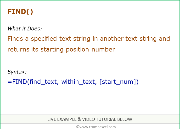
Excel FIND function can be used when you want to locate a text string within another text string and find its position.
What it Returns
It returns a number that represents the starting position of the string you are finding in another string.
Syntax
=FIND(find_text, within_text, [start_num])
Input Arguments
- find_text – the text or string that you need to find.
- within_text – the text within which you want to find the find_text argument.
- [start_num] – a number that represents the position from which you want the search to begin. If you omit it, it starts from the beginning.
Additional Notes
- If the start number is not specified, then it starts looking from the beginning of the string.
- Excel FIND function is case-sensitive. If you want to do a case-insensitive search, use Excel SEARCH function.
- Excel FIND function cannot handle wildcard characters. If you want to use wildcard characters, use the Excel SEARCH function.
- It returns a #VALUE! error if the searched string is not found in the text.
Excel FIND Function – Examples
Here are four examples of using Excel FIND function:
Searching for a Word in a Text String (from the beginning)
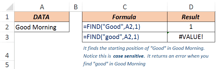
In the above example, when you look for the word Good in the text Good Morning, it returns 1, which is the position of the starting point of the searched word.
Note that Excel FIND function is case-sensitive. When you use good instead of Good, it returns a #VALUE! error.
If you are looking for a case-insensitive search, use Excel SEARCH function.
Finding a Word in a Text String (with a specified beginning)
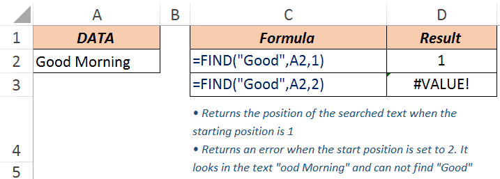
The third argument in the FIND function is the position within the text from where you want to start the search. In the example above, the function returns 1 when you search for the text Good in Good Morning and the starting position is 1.
However, it returns an error when you make it start at 2. Hence, it looks for the text Good in ood Morning. Since it can not find it, it returns an error.
Note: If you skip the last argument and don’t provide the starting position, by default it takes it as 1.
When there are Multiple Occurrence of the Searched Text
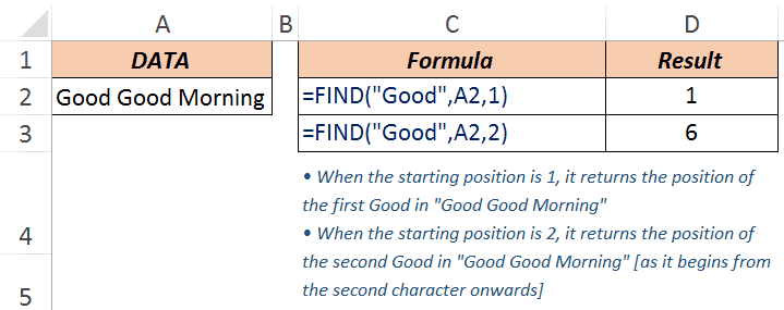
Excel FIND function starts looking in the specified text from the specified position. In the above example, when you look for the text Good in Good Good Morning with the starting position as 1, it returns 1, as it finds it at the beginning.
When you start the search from the second character onwards, it returns 6, as it finds the matching text at the sixth position.
Extracting Everything to the Left a Specified Character/String
Suppose you have the email ids do some superheroes as shown below and you want to extract only the username part (which would be the characters before the @).
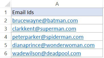
Below is the formula that will find the position of ‘@’ in each email id and extract all the characters to the left of it:
=LEFT(A2,FIND(“@”,A2,1)-1)

The FIND function in this formula gives the position of the ‘@’ character. The LEFT function that uses this position to extract the username.
For example, in the case of brucewayne@batman.com, the FIND function returns 11. LEFT function then uses FIND(“@”,A2,1)-1 as the second argument to get the username.
Note that 1 is subtracted from the value returned by the FIND function as we want to exclude the @ from the result of the LEFT function.
Excel FIND Function – VIDEO
Related Excel Functions:
- Excel LOWER Function.
- Excel UPPER Function.
- Excel PROPER Function.
- Excel REPLACE Function.
- Excel SEARCH Function.
- Excel SUBSTITUTE Function.
You May Also Like the Following Tutorials:
- How to Quickly Find and Remove Hyperlinks in Excel.
- How to Find Merged Cells in Excel.
- How to Find and Remove Duplicates in Excel.
- Using Find and Replace in Excel.
Содержание
- FIND, FINDB functions
- Description
- Syntax
- Remarks
- Examples
- In Excel find and return next value that meets the criteria
- FIND Function
- Related functions
- Summary
- Purpose
- Return value
- Arguments
- Syntax
- Usage notes
- Basic Example
- Case-sensitive
- TRUE or FALSE result
- Start number
- Wildcards
- If cell contains
- How to Return Cell Address Instead of Value in Excel (Easy Formula)
- Lookup And Return Cell Address Using the ADDRESS Function
- Lookup And Return Cell Address Using the CELL Function
- Excel — Find a value in an array and return the contents of the corresponding column
- 4 Answers 4
FIND, FINDB functions
This article describes the formula syntax and usage of the FIND and FINDB functions in Microsoft Excel.
Description
FIND and FINDB locate one text string within a second text string, and return the number of the starting position of the first text string from the first character of the second text string.
These functions may not be available in all languages.
FIND is intended for use with languages that use the single-byte character set (SBCS), whereas FINDB is intended for use with languages that use the double-byte character set (DBCS). The default language setting on your computer affects the return value in the following way:
FIND always counts each character, whether single-byte or double-byte, as 1, no matter what the default language setting is.
FINDB counts each double-byte character as 2 when you have enabled the editing of a language that supports DBCS and then set it as the default language. Otherwise, FINDB counts each character as 1.
The languages that support DBCS include Japanese, Chinese (Simplified), Chinese (Traditional), and Korean.
Syntax
FIND(find_text, within_text, [start_num])
FINDB(find_text, within_text, [start_num])
The FIND and FINDB function syntax has the following arguments:
Find_text Required. The text you want to find.
Within_text Required. The text containing the text you want to find.
Start_num Optional. Specifies the character at which to start the search. The first character in within_text is character number 1. If you omit start_num, it is assumed to be 1.
FIND and FINDB are case sensitive and don’t allow wildcard characters. If you don’t want to do a case sensitive search or use wildcard characters, you can use SEARCH and SEARCHB.
If find_text is «» (empty text), FIND matches the first character in the search string (that is, the character numbered start_num or 1).
Find_text cannot contain any wildcard characters.
If find_text does not appear in within_text, FIND and FINDB return the #VALUE! error value.
If start_num is not greater than zero, FIND and FINDB return the #VALUE! error value.
If start_num is greater than the length of within_text, FIND and FINDB return the #VALUE! error value.
Use start_num to skip a specified number of characters. Using FIND as an example, suppose you are working with the text string «AYF0093.YoungMensApparel». To find the number of the first «Y» in the descriptive part of the text string, set start_num equal to 8 so that the serial-number portion of the text is not searched. FIND begins with character 8, finds find_text at the next character, and returns the number 9. FIND always returns the number of characters from the start of within_text, counting the characters you skip if start_num is greater than 1.
Examples
Copy the example data in the following table, and paste it in cell A1 of a new Excel worksheet. For formulas to show results, select them, press F2, and then press Enter. If you need to, you can adjust the column widths to see all the data.
Источник
In Excel find and return next value that meets the criteria
Have a seemingly simple question that I just don’t know how to fix. These are the excel columns:
# is the comment sign. bewtween ** ** is highlight
The key is to find a value in ‘number’ column with current value being 1 and next one being 0 (call it end point), and then look for next value in same column with current value being 1 and previous one being 0 (call start point). Between each start point and end point is a short line.
Then in ‘result’ column (can go to any row), calculate a result of function based on existing values (just name it functionA ) and when the calculated result resultA reaches a threshold value 3, I will highlight all the values involved in these two lines and remove them later on. As seen in the data. resultA is calculated using the value of points (ID2 and ID5) in ‘number ’ column, and it reaches the threshold , so all points in these two lines are highlighted in bold font. resultB doesn’t reach the threshold, so points in line3 are not highlighted. I cannot think of how to write function that fill in the column ‘result’ . Any idea?
Now the question has simplified: the H column is my result ! And what i need to do is just find the H cell that is small than 100 (the cell highlighted is 48 so it meets criteria), and highlight all data that have consecutive 1 values in K column as 1,1,1. and closest to the current row. as being highlighted in the image. This selection is the final step.
H column in worksheet corresponds to result column in the first excel dataset. Now just look at the worksheet.
this row 13 (with H value of 48.9) is where a end point is in—from K column you can see a series of 1.. and that tells you where is end and starting point of each list made of 1.
so 48.09 on H13 is calculated using the G13 and G15, which are the G column value of end point of current list and starting point of next list. so K13=function(G13,G15)
what needs to do is, if this value in H Follow
Источник
FIND Function

Summary
The Excel FIND function returns the position (as a number) of one text string inside another. When the text is not found, FIND returns a #VALUE error.
Purpose
Return value
Arguments
- find_text — The substring to find.
- within_text — The text to search within.
- start_num — [optional] The starting position in the text to search. Optional, defaults to 1.
Syntax
Usage notes
The FIND function returns the position (as a number) of one text string inside another. If there is more than one occurrence of the search string, FIND returns the position of the first occurrence. When the text is not found, FIND returns a #VALUE error. Also note, when find_text is empty, FIND returns 1. FIND does not support wildcards, and is always case-sensitive. Use the SEARCH function to find the position of text without case-sensitivity and with wildcard support.
Basic Example
The FIND function is designed to look inside a text string for a specific substring. When FIND locates the substring, it returns a position of the substring in the text as a number. If the substring is not found, FIND returns a #VALUE error. For example:
Note that text values entered directly into FIND must be enclosed in double-quotes («»).
Case-sensitive
The FIND function always case-sensitive:
TRUE or FALSE result
To force a TRUE or FALSE result, nest the FIND function inside the ISNUMBER function. ISNUMBER returns TRUE for numeric values and FALSE for anything else. If FIND locates the substring, it returns the position as a number, and ISNUMBER returns TRUE:
If FIND doesn’t locate the substring, it returns an error, and ISNUMBER returns FALSE.
Start number
The FIND function has an optional argument called start_num, that controls where FIND should begin looking for a substring. To find the first match of «the» in any combination of upper or lowercase, you can omit start_num, which defaults to 1:
To start searching at character 5, enter 4 for start_num:
Wildcards
The FIND function does not support wildcards. See the SEARCH function.
If cell contains
To return a custom result with the SEARCH function, use the IF function like this:
Instead of returning TRUE or FALSE, the formula above will return «Yes» if substring is found and «No» if not.
Источник
How to Return Cell Address Instead of Value in Excel (Easy Formula)
When using lookup formulas in Excel (such as VLOOKUP, XLOOKUP, or INDEX/MATCH), the intent is to find the matching value and get that value (or a corresponding value in the same row/column) as the result.
But in some cases, instead of getting the value, you may want the formula to return the cell address of the value.
This could be especially useful if you have a large data set and you want to find out the exact position of the lookup formula result.
There are some functions in Excel that designed to do exactly this.
In this tutorial, I will show you how you can find and return the cell address instead of the value in Excel using simple formulas.
This Tutorial Covers:
Lookup And Return Cell Address Using the ADDRESS Function
The ADDRESS function in Excel is meant to exactly this.
It takes the row and the column number and gives you the cell address of that specific cell.
Below is the syntax of the ADDRESS function:
- row_num: Row number of the cell for which you want the cell address
- column_num: Column number of the cell for which you want the address
- [abs_num]: Optional argument where you can specify whether want the cell reference to be absolute, relative, or mixed.
- [a1]: Optional argument where you can specify whether you want the reference in the R1C1 style or A1 style
- [sheet_text]: Optional argument where you can specify whether you want to add the sheet name along with the cell address or not
Now, let’s take an example and see how this works.
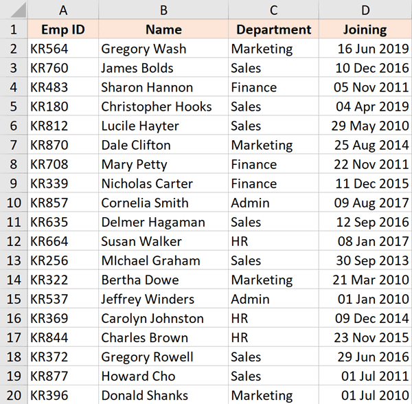
Suppose there is a dataset as shown below, where I have the Employee id, their name, and their department, and I want to quickly know the cell address that contains the department for employee id KR256.
Below is the formula that will do this:
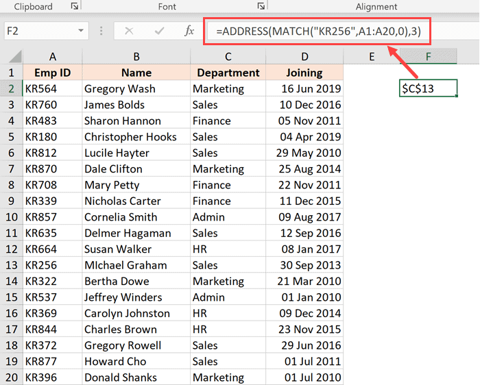
In the above formula, I have used the MATCH function to find out the row number that contains the given employee id.
And since the department is in column C, I have used 3 as the second argument.
This formula works great, but it has one drawback – it won’t work if you add the row above the dataset or a column to the left of the dataset.
This is because when I specify the second argument (the column number) as 3, it’s hard-coded and won’t change.
In case I add any column to the left of the dataset, the formula would count 3 columns from the beginning of the worksheet and not from the beginning of the dataset.
So, if you have a fixed dataset and need a simple formula, this will work fine.
But if you need this to be more fool-proof, use the one covered in the next section.
Lookup And Return Cell Address Using the CELL Function
While the ADDRESS function was made specifically to give you the cell reference of the specified row and column number, there is another function that also does this.
It’s called the CELL function (and it can give you a lot more information about the cell than the ADDRESS function).
Below is the syntax of the CELL function:
- info_type: the information about the cell you want. This could be the address, the column number, the file name, etc.
- [reference]: Optional argument where you can specify the cell reference for which you need the cell information.
Now, let’s see an example where you can use this function to look up and get the cell reference.
Suppose you have a dataset as shown below, and you want to quickly know the cell address that contains the department for employee id KR256.
Below is the formula that will do this:
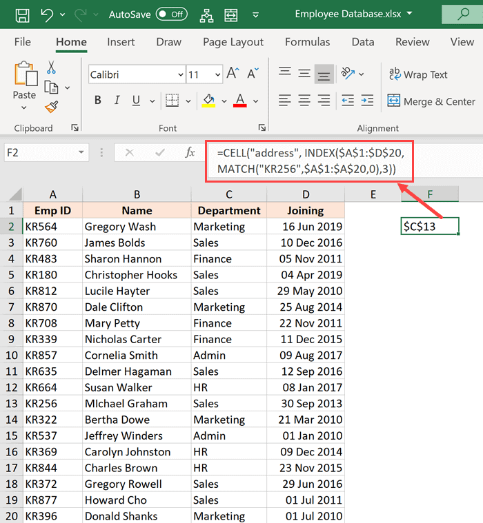
The above formula is quite straightforward.
I have used the INDEX formula as the second argument to get the department for the employee id KR256.
And then simply wrapped it within the CELL function and asked it to return the cell address of this value that I get from the INDEX formula.
Now here is the secret to why it works – the INDEX formula returns the lookup value when you give it all the necessary arguments. But at the same time, it would also return the cell reference of that resulting cell.
In our example, the INDEX formula returns “Sales” as the resulting value, but at the same time, you can also use it to give you the cell reference of that value instead of the value itself.
Normally, when you enter the INDEX formula in a cell, it returns the value because that is what it’s expected to do. But in scenarios where a cell reference is required, the INDEX formula will give you the cell reference.
In this example, that’s exactly what it does.
And the best part about using this formula is that it is not tied to the first cell in the worksheet. This means that you can select any data set (which could be anywhere in the worksheet), use the INDEX formula to do a regular look up and it would still give you the correct address.
And if you insert an additional row or column, the formula would adjust accordingly to give you the correct cell address.
So these are two simple formulas that you can use to look up and find and return the cell address instead of the value in Excel.
I hope you found this tutorial useful.
Other Excel tutorials you may also like:
Источник
Excel — Find a value in an array and return the contents of the corresponding column
I am trying to find a value within an array and then return the value in a specific row in the corresponding column.
In the example below, I need to know which bay the Chevrolet is in:
I am looking for Chevrolet in the array C2:E5. Once it determines that the Chevrolet is in Column D, I need for it to return the value in D1. If it was in column E, I need it to return the value in E1.
Any help would be greatly appreciated. Thank you so much in advance.

4 Answers 4
Try this Array Formula:
or if you are sure that each column contains exactly what’s being searched it can be written like this:
Enter formula in any cell by pressing Ctrl + Shitf + Enter .
How does it work?
Our ultimate goal is to find the Column that contains the match:
- First we did the search for the match using this formula: SEARCH(A1,$C$1:$E$5) . It just checks if any of the entries matched A1. Actually, it can be simplified to $C$1:$E$5=A1 but I’m not sure if all entries in each column match exactly what’s in A1.
- That formula will produce an array of values when entered as array formula. Something like: . The result will be array of number(s) and error (if non was found). But we don’t want that, else we will be returning error everytime.
- We then use IF(NOT(ISERROR(SEARCH(A1,$C$1:$E$5))),COLUMN($A:$C),99^99) . This formula returns the Column Number if there is a match and a relatively huge number 99^99 otherwise. Result would be: <99^99, 99^99, 99^99, 2, . 99^99>.
- And we are close to what we need since we already have an array of Column and huge number. We just use SMALL to return the smallest number which in my opinion is the lowest Column Number where a match is found. So SMALL(IF(NOT(ISERROR(SEARCH(A1,$C$1:$E$5))),COLUMN($A:$C),99^99),1) would return 2. Which is the column where Chevrolet is referenced at $C$1:$E$1.
- Since we already have the column number we simply use INDEX Function which is: INDEX($C$1:$E$5,1,2) .
Note: 99^99 can be any relatively large number. Not necessarily 99^99 . Actual 16385(max column number in Excel 2007 and up + 1) can be used.
Result: 
Источник