Excel find name in table

Summary

This step-by-step article describes how to find data in a table (or range of cells) by using various built-in functions in Microsoft Excel. You can use different formulas to get the same result.

Create the Sample Worksheet

This article uses a sample worksheet to illustrate Excel built-in functions. Consider the example of referencing a name from column A and returning the age of that person from column C. To create this worksheet, enter the following data into a blank Excel worksheet.

You will type the value that you want to find into cell E2. You can type the formula in any blank cell in the same worksheet.

	A	B	C	D	E
1	Name	Dept	Age		Find Value
2	Henry	501	28		Mary
3	Stan	201	19
4	Mary	101	22
5	Larry	301	29

Term Definitions

This article uses the following terms to describe the Excel built-in functions:

Term	Definition	Example
Table Array	The whole lookup table	A2:C5
Lookup_Value	The value to be found in the first column of Table_Array.	E2
Lookup_Array -or- Lookup_Vector	The range of cells that contains possible lookup values.	A2:A5
Col_Index_Num	The column number in Table_Array the matching value should be returned for.	3 (third column in Table_Array)
Result_Array -or- Result_Vector	A range that contains only one row or column. It must be the same size as Lookup_Array or Lookup_Vector.	C2:C5
Range_Lookup	A logical value (TRUE or FALSE). If TRUE or omitted, an approximate match is returned. If FALSE, it will look for an exact match.	FALSE
Top_cell	This is the reference from which you want to base the offset. Top_Cell must refer to a cell or range of adjacent cells. Otherwise, OFFSET returns the #VALUE! error value.
Offset_Col	This is the number of columns, to the left or right, that you want the upper-left cell of the result to refer to. For example, «5» as the Offset_Col argument specifies that the upper-left cell in the reference is five columns to the right of reference. Offset_Col can be positive (which means to the right of the starting reference) or negative (which means to the left of the starting reference).

Functions

LOOKUP()

The LOOKUP function finds a value in a single row or column and matches it with a value in the same position in a different row or column.

The following is an example of LOOKUP formula syntax:

   =LOOKUP(Lookup_Value,Lookup_Vector,Result_Vector)

The following formula finds Mary’s age in the sample worksheet:

   =LOOKUP(E2,A2:A5,C2:C5)

The formula uses the value «Mary» in cell E2 and finds «Mary» in the lookup vector (column A). The formula then matches the value in the same row in the result vector (column C). Because «Mary» is in row 4, LOOKUP returns the value from row 4 in column C (22).

NOTE: The LOOKUP function requires that the table be sorted.

For more information about the LOOKUP function, click the following article number to view the article in the Microsoft Knowledge Base:
 

How to use the LOOKUP function in Excel

VLOOKUP()

The VLOOKUP or Vertical Lookup function is used when data is listed in columns. This function searches for a value in the left-most column and matches it with data in a specified column in the same row. You can use VLOOKUP to find data in a sorted or unsorted table. The following example uses a table with unsorted data.

The following is an example of VLOOKUP formula syntax:

    =VLOOKUP(Lookup_Value,Table_Array,Col_Index_Num,Range_Lookup)

The following formula finds Mary’s age in the sample worksheet:

   =VLOOKUP(E2,A2:C5,3,FALSE)

The formula uses the value «Mary» in cell E2 and finds «Mary» in the left-most column (column A). The formula then matches the value in the same row in Column_Index. This example uses «3» as the Column_Index (column C). Because «Mary» is in row 4, VLOOKUP returns the value from row 4 in column C (22).

For more information about the VLOOKUP function, click the following article number to view the article in the Microsoft Knowledge Base:
 

How to Use VLOOKUP or HLOOKUP to find an exact match

INDEX() and MATCH()

You can use the INDEX and MATCH functions together to get the same results as using LOOKUP or VLOOKUP.

The following is an example of the syntax that combines INDEX and MATCH to produce the same results as LOOKUP and VLOOKUP in the previous examples:

    =INDEX(Table_Array,MATCH(Lookup_Value,Lookup_Array,0),Col_Index_Num)

The following formula finds Mary’s age in the sample worksheet:

    =INDEX(A2:C5,MATCH(E2,A2:A5,0),3)

The formula uses the value «Mary» in cell E2 and finds «Mary» in column A. It then matches the value in the same row in column C. Because «Mary» is in row 4, the formula returns the value from row 4 in column C (22).

NOTE: If none of the cells in Lookup_Array match Lookup_Value («Mary»), this formula will return #N/A.
For more information about the INDEX function, click the following article number to view the article in the Microsoft Knowledge Base:

How to use the INDEX function to find data in a table

OFFSET() and MATCH()

You can use the OFFSET and MATCH functions together to produce the same results as the functions in the previous example.

The following is an example of syntax that combines OFFSET and MATCH to produce the same results as LOOKUP and VLOOKUP:

   =OFFSET(top_cell,MATCH(Lookup_Value,Lookup_Array,0),Offset_Col)

This formula finds Mary’s age in the sample worksheet:

   =OFFSET(A1,MATCH(E2,A2:A5,0),2)

The formula uses the value «Mary» in cell E2 and finds «Mary» in column A. The formula then matches the value in the same row but two columns to the right (column C). Because «Mary» is in column A, the formula returns the value in row 4 in column C (22).

For more information about the OFFSET function, click the following article number to view the article in the Microsoft Knowledge Base:
 

How to use the OFFSET function

To search for text or numbers, follow these steps:

1. Click the Home tab.
2. Click the Find & Select icon in the Editing group.
3. Click Find.
4. Click in the Find What text box and type the text or number you want to find.
5. Click one of the following:
6. Click Close to make the Find and Replace dialog box go away.

How do you search for names in Excel?

To find something, press Ctrl+F, or go to Home > Find & Select > Find.

1. In the Find what: box, type the text or numbers you want to find.
2. Click Find Next to run your search.
3. You can further define your search if needed: Within: To search for data in a worksheet or in an entire workbook, select Sheet or Workbook.

How to Extract a List of Named Ranges in Excel

1. Select a blank cell in your workbook.
2. Under the Formulas menu item, select Use in Formula.
3. Select Paste Names… at the bottom of the list.

Can Excel recognize names?

Similarly, in Microsoft Excel, you can give a human-readable name to a single cell or a range of cells, and refer to those cells by name rather than by reference.

How do I see table names in Excel?

In Excel 2010 you can also see the Table name by choosing Formulas > Name Manager. In Excel 2011 you choose Insert > Name > Define to see the Table name. Knowing a Table’s name is important in Excel. It’s the first step in understanding structured Table data.

Where is name manager in Excel?

Formulas tab
To open the Name Manager dialog box, on the Formulas tab, in the Defined Names group, click Name Manager. One of the following: A defined name, which is indicated by a defined name icon.

How do I find similar names in Excel?

Find and remove duplicates

1. Select the cells you want to check for duplicates.
2. Click Home > Conditional Formatting > Highlight Cells Rules > Duplicate Values.
3. In the box next to values with, pick the formatting you want to apply to the duplicate values, and then click OK.

What are the rules for naming workbook?

Excel Worksheet Naming Rules and Tips

• ► Two worksheets cannot have the same name, regardless of upper or lowercase.
• ► A worksheet name cannot cannot exceed 31 characters.
• ► A worksheet name cannot be left blank.
• ► A worksheet cannot be named history in either lower or uppercase.

What is the shortcut to name a cell in Excel?

When naming a cell or range, it can only be one word with no spaces. In Excel, use the shortcut key Ctrl + F3 to open the Name Manager. In the Name Manager, you can create, edit, and delete any Excel names. Once a name is created, you can use the shortcut key F3 to insert any name.

What is an Xlookup in Excel?

Use the XLOOKUP function to find things in a table or range by row.With XLOOKUP, you can look in one column for a search term, and return a result from the same row in another column, regardless of which side the return column is on.

How do I find out a table name?

II. Find Table By Table Name Using Filter Settings in Object Explores

1. In the Object Explorer in SQL Server Management Studio, go to the database and expand it.
2. Right Click the Tables folder and select Filter in the right-click menu.
3. Under filter, select Filter Settings.

How does a VLOOKUP work?

The VLOOKUP function performs a vertical lookup by searching for a value in the first column of a table and returning the value in the same row in the index_number position.As a worksheet function, the VLOOKUP function can be entered as part of a formula in a cell of a worksheet.

How do I match names from one spreadsheet to another?

Select both columns of data that you want to compare. On the Home tab, in the Styles grouping, under the Conditional Formatting drop down choose Highlight Cells Rules, then Duplicate Values. On the Duplicate Values dialog box select the colors you want and click OK. Notice Unique is also a choice.

How do you automatically name a sheet in Excel?

You can also access the option to rename sheets through the Excel ribbon:

1. Click the Home tab.
2. In the Cell group, click on the ‘Format’ option.
3. Click on the Rename Sheet option. This will get the sheet name into edit mode.
4. Enter the name that you want for the sheet.

Where is the sheet tab in Excel?

bottom
The worksheet tab can be found at the bottom of every excel worksheet tab.

What is reserved name in Excel?

Whenever you try to name a worksheet as History, Excel will return a warning message that ‘History is a reserved name’. History is a reserved name for the sheet meant for ‘tracking changes between shared workbooks’. A dialog called Highlight Changes will be activated.

How do you make a cell named?

Naming cells

1. Select the cell or cell range that you want to name. You also can select noncontiguous cells (press Ctrl as you select each cell or range).
2. On the Formulas tab, click Define Name in the Defined Names group.
3. In the Name text box, type up to a 255-character name for the range.
4. Click OK.

How do I select a cell name in Excel?

Use names in formulas

1. Select a cell and enter a formula.
2. Place the cursor where you want to use the name in that formula.
3. Type the first letter of the name, and select the name from the list that appears. Or, select Formulas > Use in Formula and select the name you want to use.
4. Press Enter.

How do I enable Xlookup?

1. Position the cell cursor in cell E4 of the worksheet.
2. Click the Lookup & Reference option on the Formulas tab followed by XLOOKUP near the bottom of the drop-down menu to open its Function Arguments dialog box.
3. Click cell D4 in the worksheet to enter its cell reference into the Lookup_value argument text box.

How is Xlookup different from VLOOKUP?

XLOOKUP defaults to an exact match. VLOOKUP defaults to an “approximate” match, requiring that you add the “false” argument at the end of your VLOOKUP to perform an exact match.XLOOKUP can perform horizontal or vertical lookups. The XLOOKUP replaces both the VLOOKUP and HLOOKUP.

How do I get Xlookup?

Since XLOOKUP will likely only be available to Office 365 users, one way to get it is to upgrade to Office 365. If you already have Office 365 Home, Personal, or University edition, you already have access to XLOOKUP. All you need to do is join the Office Insider program.

Функция НАЙТИ (FIND) в Excel используется для поиска текстового значения внутри строчки с текстом и указать порядковый номер буквы с которого начинается искомое слово в найденной строке.

Что возвращает функция

Возвращает числовое значение, обозначающее стартовую позицию текстовой строчки внутри другой текстовой строчки.

Синтаксис

=FIND(find_text, within_text, [start_num]) — английская версия

=НАЙТИ(искомый_текст;просматриваемый_текст;[нач_позиция]) — русская версия

Аргументы функции

• find_text (искомый_текст) — текст или строка которую вы хотите найти в рамках другой строки;
• within_text (просматриваемый_текст) — текст, внутри которого вы хотите найти аргумент find_text (искомый_текст);
• [start_num] ([нач_позиция]) — число, отображающее позицию, с которой вы хотите начать поиск. Если аргумент не указать, то поиск начнется сначала.

Дополнительная информация

• Если стартовое число не указано, то функция начинает поиск искомого текста с начала строки;
• Функция НАЙТИ чувствительна к регистру. Если вы хотите сделать поиск без учета регистра, используйте функцию SEARCH в Excel;
• Функция не учитывает подстановочные знаки при поиске. Если вы хотите использовать подстановочные знаки для поиска, используйте функцию SEARCH в Excel;
• Функция каждый раз возвращает ошибку, когда не находит искомый текст в заданной строке.

Примеры использования функции НАЙТИ в Excel

Пример 1. Ищем слово в текстовой строке (с начала строки)

На примере выше мы ищем слово «Доброе» в словосочетании «Доброе Утро». По результатам поиска, функция выдает число «1», которое обозначает, что слово «Доброе» начинается с первой по очереди буквы в, заданной в качестве области поиска, текстовой строке.

Обратите внимание, что так как функция НАЙТИ в Excel чувствительна к регистру, вы не сможете найти слово «доброе» в словосочетании «Доброе утро», так как оно написано с маленькой буквы. Для того, чтобы осуществить поиска без учета регистра следует пользоваться функцией SEARCH.

Пример 2. Ищем слово в текстовой строке (с заданным порядковым номером старта поиска)

Третий аргумент функции НАЙТИ указывает позицию, с которой функция начинает поиск искомого значения. На примере выше функция возвращает число «1» когда мы начинаем поиск слова «Доброе» в словосочетании «Доброе утро» с начала текстовой строки. Но если мы зададим аргумент функции start_num (нач_позиция) со значением «2», то функция выдаст ошибку, так как начиная поиск со второй буквы текстовой строки, она не может ничего найти.

Если вы не укажете номер позиции, с которой функции следует начинать поиск искомого аргумента, то Excel по умолчанию начнет поиск с самого начала текстовой строки.

Пример 3. Поиск текстового значения внутри текстовой строки с дублированным искомым значением

На примере выше мы ищем слово «Доброе» в словосочетании «Доброе Доброе утро». Когда мы начинаем поиск слова «Доброе» с начала текстовой строки, то функция выдает число «1», так как первое слово «Доброе» начинается с первой буквы в словосочетании «Доброе Доброе утро».

Но, если мы укажем в качестве аргумента start_num (нач_позиция) число «2» и попросим функцию начать поиск со второй буквы в заданной текстовой строке, то функция выдаст число «6», так как Excel находит искомое слово «Доброе» начиная со второй буквы словосочетания «Доброе Доброе утро» только на 6 позиции.

When working with the names dataset in Excel, often there is a need to slice and dice the dataset and extract a part of it.

One common task many Excel users have to do is to extract the last name from the full name.

While it may seem like an easy task, it can get complicated (especially when you’re dealing with data that is not consistent).

In this tutorial, I will show you five different ways to extract the last name from the full name in Excel. I will cover different scenarios, where you only have the first and the last name in the dataset, or the first, middle, and last name.

So let’s get started!

Extract Last Name Using Find and Replace

Extracting the last name from a full name essentially means you’re replacing everything before the last name with a blank.

And this can easily be done using Find and Replace in Excel (and it takes less than 3 seconds).

Below I have a names data set from which I want to extract only the last name.

Below are the steps to use Find and Replace to remove everything before the last name:

1. Copy the name data from Column A and paste it in Column B. I am doing this to keep the original data intact. If you only need the last name, you can skip this step.

1. Select all the names in column B

1. Hold the Control key and press the H key (Command + H if using Mac). This will open the Find and Replace dialog box.

1. In the Find and Replace dialog box, enter the following in the Find what field: * (an asterisk symbol followed by a space character)

1. Leave the Replace with field empty/blank
2. Click on Replace All

The above steps food remove anything before the last space character, which would leave us with the last names only.

The above method would also work in case you have an inconsistent names dataset. For example, if you have names that may or may not have a middle name/initial, or may have a prefix such as Mr or Ms. The only condition is that the last name should be at the end of the name

How does this work?

In the ‘Find what’ field in the Find and Replace dialog box, I have used an asterisk sign (*) followed by a space character.

Asterisk is a wild card character that represents any number of characters in Excel.

So when I ask it to find an asterisk followed by the space character, it will find the last space character in the cell and everything before that space character would be considered a part of the asterisk.

And when I replace it with a blank, everything before the last space character is removed.

Note: For this method to work you need to make sure that there are no trailing spaces in your data. In case there is a space character after the last name, doing the above Find and Replace operation would remove everything from the cell. To make sure there are no trailing spaces, you can use the TRIM formula (read – how to remove trailing spaces in Excel)

Extract Last Name Using Formulas (When you Have Only First and Last name)

Suppose you have a data set as shown below where you have the first name and the last name in column A, and you only want to extract the last name from it.

Below is the formula that will do that:

=RIGHT(A2,LEN(TRIM(A2))-FIND(" ",TRIM(A2)))

Let me quickly explain how this formula works.

The above formula uses the FIND function to get the position of the space character in the name.

Since the position of the space character would be between the first and the last name, once we have the position of the space character, we can use that to extract everything to the right of it (which would be the last name)

But how many characters from the right should it extract?

Since we have the position of the space character, we can subtract that value from the length of the name (which is given by the LEN function). This tells us how many characters are there after the space character in the name.

And this value is then used in the RIGHT formula to extract the last name from the full name.

Note that I have used TRIM(A2) instead of A2 in this formula. This is because there is a possibility that the cells containing the names may have leading, trailing, or double spaces in them. Using the TRIM function makes sure that all these extra spaces are ignored and only one space character between the first name and the last name is considered.

Extract Last Name Using Formulas (When you Have First, Middle, and Last name)

In case you have the first, middle, and last name, the formula becomes a little bit longer.

Below I have a data set where I have the first, middle, last name in column A, and I want to extract the last name from it.

Here is a formula that can do that:

=RIGHT(TRIM(A2),LEN(TRIM(A2))-SEARCH(" ",TRIM(A2),SEARCH(" ",TRIM(A2))+1))

The above function uses the same concept where we have to find out the position of the last space character, and then extract everything to the right of that space character.

But since there are two space characters, in this case, the challenge is to find out the position of this second space character.

To do this, I have used the below-nested SEARCH function (i.e., Search function within a search function)

=SEARCH(" ",TRIM(A2),SEARCH(" ",TRIM(A2))+1)

This part of the formula gives us the position of the second space character, which is then used within the RIGHT formula to extract the last name.

Note that this formula would only work when you have a consistent names dataset – i.e., all the names have the first, middle, and last names.

In case you have a mix of names where some may have middle names but some may not, this formula is not going to work.

If that is the case, use the formula in the next section.

When You Have Incosistent Data (Names with and Without Middle Name)

Below I have a named data set where the format is not consistent – in some cells, we only have the first and last name, and in some cells, there are a middle name and/or prefixes as well.

While you can still use excel formulas to extract the last name in this case, the formula we’ll get a little bit complicated.

Below is the formula that will extract the last name in this inconsistent data set:

=RIGHT(SUBSTITUTE(A2," ","|",LEN(A2)-LEN(SUBSTITUTE(A2," ",""))),LEN(SUBSTITUTE(A2," ","|",LEN(A2)-LEN(SUBSTITUTE(A2," ",""))))-FIND("|",SUBSTITUTE(A2," ","|",LEN(A2)-LEN(SUBSTITUTE(A2," ","")))))

Also read: How to Switch First and Last Name in Excel with Comma?

Extract Last Name using Flash Fill

Another really fast way to extract the last name from full names is by using the Flash Fill feature in Excel.

Introduced in Excel 2013, Flash Fill works by identifying patterns based on user input and giving you the same results for all the cells in the column.

Below I have a data set where I have the names in column A and I want to extract the last name in column B.

Here are the steps to do this Flash Fill:

1. In cell B2, manually enter the last name from the name in cell A2

1. Select the range in column B where you want the last names (B2:B10 in this example)

1. Hold the Control key and press the E key (or Command + E if using Mac)

Note: You can also get the same option when you go to the Home tab, click on the Fill icon, and then click on Flash Fill

The above steps would fill the selected range with the last names from names in Column A.

As I mentioned, Flash Fill works by identifying the pattern in one or two cells where you have manually entered the data and then replicates it for all the other select cells.

In this example, when I entered “Hans” in cell B2, and then used Flash Fill, it recognized that I’m trying to extract the last word from the text string in column A. So we did the same for all the cells I selected.

In case you have a dataset where you have a mix of names with and without a middle name, you can still use Flash Fill to extract the last name.

This is because the pattern that the flash fill has identified is to extract the last word from the text string, so it doesn’t matter how many words are there, it will give you the last name in any case.

Caution: While the flash fill method has worked perfectly in our case, its accuracy is dependent on how well it can identify the pattern. In some cases, it may not be able to identify the right pattern, so it’s important that you double-check the data to make sure it’s correct. In some cases, you may need to enter the data in two or three cells for flash fill to identify the pattern correctly

Compared with the formula method covered above, the flash fill method is a lot faster and more convenient.

One big difference however is that the result of the formula method is dynamic, which means that in case you change the original name, the result in the cell that has the formula would also update.

In the case of Flash Fill, you will have to repeat the same process again to get the updated data

Extract Last Name Using Power Query

If you want to automate the process of extracting the last names from full names, Power Query is the way to go.

For example, if you often have a need to separate names in Excel or to extract the first or last name, you can do that once using Power Query, and the next time you need to do it again, you can simply refresh the query with a single click.

Below I have a data set of names and I want to extract the last name from these. Note that I have a mix of names where there are middle names and prefixes in some of the cells.

Note: When using Power Query, it is best to convert your data into an Excel Table. Doing this would make it a lot easier to work with Power Query, and also allow you to perform the same steps with a single click the next time you add new data set.

To convert your data into an Excel Table, select the data and use the keyboard shortcut Control + T (or Command + T if using Mac)

Below are the steps to use Power Query to get the last name from this dataset:

1. Select any cell in the dataset
2. Click the Data tab in the ribbon

1. In the ‘Get and Transform Data’ group, click on ‘From Selection’. This will open the Power Query editor

1. In the PQ Editor, right-click on the column header

1. Go to the ‘Split Column’ option
2. Click on By Delimiter option.

1. In the ‘Split Column by Delimiter’ dilaog box, select Space as the delimiter (if not selected already)

1. In the Split at options, select ‘Right-most delimiter’

1. Click OK. This will close the dialog box and you will see the result in the PQ Editor

1. Rename the columns the way you want (I am going with ‘Full Name’ and ‘Last Name’)

1. Click on Close and Load option in the ribbon

The above steps would insert a new worksheet in your workbook that would have the resulting table.

Note that in the above example, the first name column has the first name as well as the middle name in some cases. In case you only want the last names, you can delete the first column in Power Query, so it will only give you the last name column as the result in the worksheet.

Now if you’re thinking that this is a long method and you’re better off using Flash Fill or formula method instead, you’re probably right.

The scenario where Power Query really shines is when you get a file that has the data and you need to do multiple modifications to it (say delete some columns, delete blank rows, extract the last name, etc).

The next time you get a new file, you won’t have to repeat all these steps again. simply connect your query to the new file and refresh the query.

In such scenarios, Power Query is a far better solution than using flash fill or formulas or even VBA.

So these are three different methods that you can use to extract the last name from full name in Excel. Personally, I prefer using the Flash Fill method in most cases, as it’s fast and quite reliable.

I hope you found this tutorial useful!

Other Excel tutorials you may also like:

• How to Shuffle a List of Items/Names in Excel?
• How to Combine First and Last Name in Excel)
• How to Sort by the Last Name in Excel
• Extract Usernames from Email Ids in Excel
• Separate First and Last Name in Excel (Split Names Using Formulas)
• How to Extract the First Word from a Text String in Excel

This post will guide you how to use Excel FIND function with syntax and examples in Microsoft excel.

Description

The Excel FIND function returns the position of the first text string (sub string) within another text string.

It can be used when you want to get the position of a sub string inside another text string. so it will return a number that indicates the starting position of sub string that you are searching in another text string.

The FIND function is a build-in function in Microsoft Excel and it is categorized as a Text Function.

Note: The FIND Function is case-sensitive.

The FIND function is available in Excel 2016, Excel 2013, Excel 2010, Excel 2007, Excel 2003, Excel xp, Excel 2000, Excel 2011 for Mac.

Syntax

The syntax of the FIND function is as below:

= FIND(find_text, within_text,[start_num])

Where the FIND function arguments are:

• Find_text -This is a required argument. The text  or substring that you want to find. (The string in the Find_text argument can not contain any wildcard characters)
• within_text -This is a required argument. The text string that is to be searched
• start_num-This is an optional argument. It will specify the position in within text string where the search will start. If you omit start_num value, the search will start from the first character of the within_text string, in other words, it is set to be 1 by default.  So you can use the Excel Find function to look for the specified text starting from the specified position.

Note:

• The Find function will return the position of the first character of find_text in within_text argument.
• If there are several occurrences of the find_text within another text string, it only return the position of the first occurrence.
• If the find_text is an empty string, the position of the first character in the within_text is returned.
• If the find_text string is not found in within_text, it will return the Excel #VALUE! Error.
• If start_number value is not greater than 0, it will return the #VALUE! Error value.
• As the FIND function is case-sensitive. If you want to do a search that is case-insensitive , you can use the SEARCH Function.
• The FIND function does not support wildcard characters, so if you want to use wildcard characters to find string, you can use SEARCH function in excel.

Excel Find Function Examples

The below example will show you how to use Excel FIND Text function to find the position of a sub string within text string.

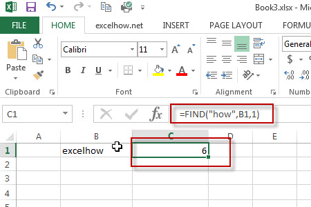
#1 To get the position of sub string “how” in cell B1, just using formula:

 =FIND("how",B1,1).

When you look for the text “how” in the Cell B1, it will return 6, which is the position of the first character of find_text “how” within the Cell B1.

#2 To get the position of sub string “how”in cell b1, starting with the third character, using formula:

=FIND("how",B1,3)

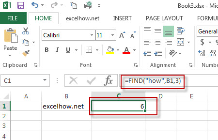
In the above example, it specified the start_num value as “3“, so you will get the position of the first character “h” of  the searched string “how”  within the value in Cell B1 when the starting position is 3. it returns 6.

The Example 1The search will start from the third character of the value in Cell B1.

#3 Finding “excel” string  in Cell B1, using the following Find formula:

=FIND("excel",B1,1)
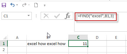
=FIND("excel",B1,3)

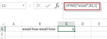
when you set the starting position as 1, it will return the position of the first “excel” string in the value of Cell B1.

When you set the starting position as 3, it will return the position of the second “excel” string in the value of Cell B1. The search will start from the third character of the value in Cell B1.

#4 Searching an empty string in Cell B1, using the following Find formula:

=FIND("",B1,1)

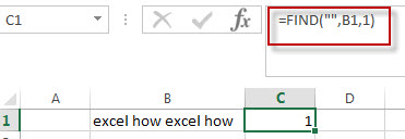
In the above example, when you look for an empty string in Cell B1 with the starting position as 1, and it will return the position of the first character of the within_ text (the value of Cell B1).

#5 Searching “word” text in Cell B1, using the following Find formula:

=FIND("word", B1,1)

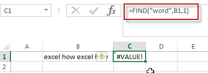
In the above example, when you look for the text “word” in Cell B1 and the string position is 1, it will return a #VALUE! error, As the searched string “word” is not found in Cell B1.

#6 Searching for a text as “excel” in Cell B1 and the starting position is a negative number.

=FIND("excel",B1,-1)

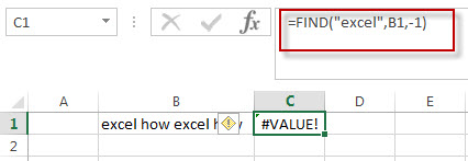
If the starting position is not greater than 0, it will return a #VALUE! Error.

#7 Searching for a string as “EXCEL” in Cell B1, using the following formula:

=FIND("EXCEL",B1,1)

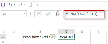
As the FIND function in excel is case-sensitive, when you look for the string “EXCEL” in Cell B1, the searched string “EXCEL” is not found, the function will return a #VALUE! error.

Frequently Asked Questions

---

Question 1:  the FIND function returns a #VALUE error when it do not find the searched text within another string.  I want to know if there is another excel function in combination with the find function to handle the error message to return the actual value, such as: -1 or throwing others exceptions via returning values, like: -1,0 or FALSE.

Answer: As mentioned above, the FIND function is case-sensitive, and it can be combined with the ISNUMBER function and IF function to create a new IF excel formula as follows:

=IF(ISNUMBER( FIND("excel",B1)), FIND("excel",B1), "not found")

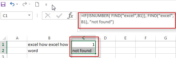
The FIND function will locate the position of the searched text “excel” within Cell B1, and the ISNUMBER function will check the result returned by the FIND function if it is a number, if TRUE, then return TRUE, otherwise , returns FALSE. then the IF will check the Boolean value returned by ISNUMBER function, If TRUE, then returns the numeric position returned by the second FIND function, If FALSE, returns “not found” string.

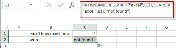
If you want a case-insensitive match and you can use the SEARCH function instead of the FIND function in the above formula:

=IF(ISNUMBER( SEARCH("excel",B1)), SEARCH("excel",B1), "not found")

Question 2: I want to extract a sub string from a string that separated by wildcard characters. I tried to use the below FIND formula to handle it. but it returned a #VALUE error message. Could you please help to check the below formula I used:

=RIGHT(B1,FIND("~**",B1))

Answer: you can use the following formula:

=TRIM(RIGHT(B1,Len(B1) - FIND("**",B1)-1))

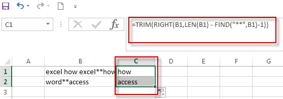
The find function will return the position of the first wildcard (**) character within a string in Cell B1. you need subtract the numeric position returned by FIND function from the length of the string in Cell B1 to get the length of sub string to the right of the wildcard character(asterisk). then the RIGHT function extracts the rightmost characters based on the length of sub string.

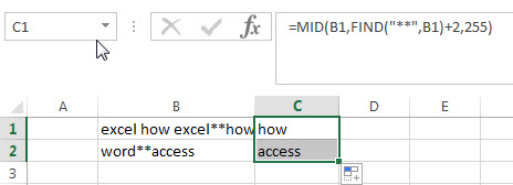
or you can use another formula to achieve the same result as follows:

=MID(B1,FIND("**",B1)+2,255)

Question 3: I am trying to extract the first word from another text string separated by space character. but it always return a #VALUE error message. I think it should be use the FIND function in combination with another function, such as: left function. but I still don’t know how to combine with those two functions to extract the first word.

Answer: right, you can create a excel formula that uses the FIND function and LEFT function. and you can use the below formula:

=IFERROR(LEFT(B1, FIND(" ",B1)-1),B1)

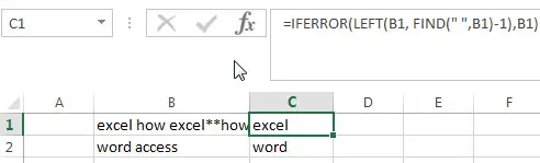
The find function returns the position of the first space character in the text string in Cell B1. the Formula “=FIND(” “,B1)-1 returns the numbers of the first word as the second arguments of the LEFT function.

If the text string in Cell B1 just only contains one word, then the find function will return #VALUE error. to handle this error, you need to use the IFERROR function, if the find function is not find the space character, then return the text string in B1. in other words, it just contains only one word in Cell B1.

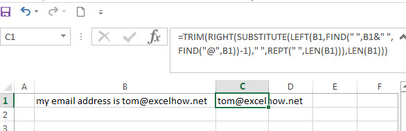
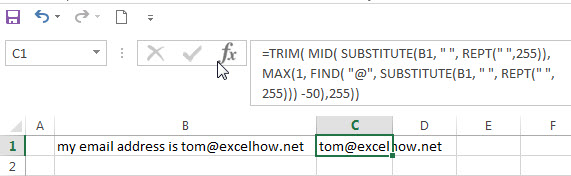
Question 4: I am trying to extract an email address from a text string in Cell B1. how to write a excel formula to achieve the result.

Answer: you can use a combination of the TRIM function, the LEFT function, the SUBSTITUTE function, the MID function, the MAX function and the REPT function to create a complex excel formula to extract email address from a string in Cell B1.

=TRIM(RIGHT(SUBSTITUTE(LEFT(B1,FIND (" ",B1&" ",FIND("@",B1))-1)," ", REPT(" ",LEN(B1))),LEN(B1)))

=TRIM( MID( SUBSTITUTE(B1, " ", REPT(" ",255)), MAX(1, FIND( "@", SUBSTITUTE(B1, " ", REPT(" ",255))) -50),255))

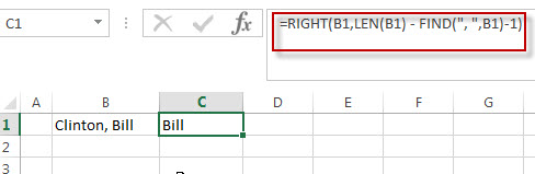
Question 5: I am trying to get the first name from a full name separated by a comma character. how to use a excel formula to extract the first name from a name as: “Last name, First name” format.

Answer: you can use a combination with the RIGHT function, the LEN function and the FIND function to create a excel formula to get the first name from a name. just using the following formula:

=RIGHT(B1,LEN(B1) - FIND(", ",B1)-1)

---

• Excel SEARCH function
  The Excel SEARCH function returns the number of the starting location of a substring in a text string.The syntax of the SEARCH function is as below:= SEARCH  (find_text, within_text,[start_num])…
• Excel Find function
  The Excel FIND function returns the position of the first text string (substring) from the first character of the second text string.The FIND function is a build-in function in Microsoft Excel and it is categorized as a Text Function.The syntax of the FIND function is as below:= FIND  (find_text, within_text,[start_num])…
• Excel ISERROR function
  The Excel ISERROR function returns TRUE if the value is any error value except #N/A. The ISERROR function is a build-in function in Microsoft Excel and it is categorized as an Information Function. The syntax of the ISERROR function is as below: = ISERROR (value) …
• Excel ISNUMBER function
  The Excel ISNUMBER function returns TRUE if the value in a cell is a numeric value, otherwise it will return FALSE.The syntax of the ISNUMBER function is as below:= ISNUMBER (value)…
• Excel RIGHT function
  The Excel RIGHT function returns a sub string (a specified number of the characters) from a text string, starting from the rightmost character.The syntax of the RIGHT function is as below:= RIGHT (text,[num_chars])…
• Excel LEN function
  The Excel LEN function returns the length of a text string (the number of characters in a text string).The LEN function is a build-in function in Microsoft Excel and it is categorized as a Text Function.The syntax of the LEN function is as below:= LEN(text)…
• Excel MID function
  The Excel MID function returns a sub string from a text string at the position that you specify. The MID function is a build-in function in Microsoft Excel and it is categorized as a Text Function. The syntax of the MID function is as below: = MID (text, start_num, num_chars) …
• Excel SUBSTITUTE function
  The Excel SUBSTITUTE function replaces a new text string for an old text string in a text string.The syntax of the SUBSTITUTE function is as below:= SUBSTITUTE  (text, old_text, new_text,[instance_num])…
• Excel LEFT function
  The Excel LEFT function returns a sub string (a specified number of the characters) from a text string, starting from the leftmost character.The LEFT function is a build-in function in Microsoft Excel and it is categorized as a Text Function.The syntax of the LEFT function is as below:= LEFT(text,[num_chars])…
• Excel REPT function
  The Excel REPT function repeats a text string a specified number of times.The REPT function is a build-in function in Microsoft Excel and it is categorized as a Text Function.The syntax of the REPT function is as below:= REPT  (text, number_times)…

More FIND Formula Examples in Excel

---

• Split Text String by Specified Character
  you should use the Left function in combination with FIND function to split the text string in excel. And we can refer to the below formula that will find the position of “-“in Cell B1 and extract all the characters to the left of the dash character “-“.=LEFT(B1,FIND(“-“,B1,1)-1).…

• Split Text String by Line Break
  When you want to split text string by line break in excel, you should use a combination of the LEFT, RIGHT, CHAR, LEN and FIND functions. The CHAR (10) function will return the line break character, the FIND function will use the returned value of the CHAR function as the first argument to locate the position of the line break character within the cell B1.…
• Split Text and Numbers in Excel
  If you want to split text and numbers, you can run the following excel formula that use the MIN function, FIND function and the LEN function within the LEFT function in excel. .…
• Get the Current Worksheet Name only
  If you want to get the current worksheet name only in excel, you can use a combination of the MID function, the CELL function and FIND function.…
• Get full File Name (workbook and worksheet) and Path
  In excel, you can get the current workbook name and it is absolute path using the CELL function.  Just refer to the following formula:=CELL(“filename”,B1).…
• Get the Current Workbook Name
  If you want to get the name of the current workbook only, you can use a combination of the MID function, the CELL function and the FIND Function…
• Get Path and Workbook name only
  If you want to get the workbook name and its path only without worksheet name, you can use a combination of the SUBSTITUTE function, the LEFT function, the CELL function and the FIND function….
• Get First Name From Full Name
  If you want to get the first name from a full name list in Column B, you can use the FIND function within LEFT function in excel. The generic formula is as follows:=LEFT(B1,FIND(” “,B1)-1).…
• Get Last Name From Full Name
  To extract the last name within a Full name in excel. You need to use a combination of the RIGHT function, the LEN function, the FIND function and the SUBSTITUTE function to create a complex formula in excel..…
• The different between FIND and SEARCH functions
  There are two big differences between FIND and SEARCH functions in excel.The FIND function is case-sensitive. And the SEARCH function is case-insensitive……
• Data Validation for Specified Text only
  If you want to check if the values that contain a specified text string in one cell, you can use a combination of the FIND function and ISNUMBER function as a formula in the Data Validation….…
• Count Cells That Contain Specific Text
  This post will discuss that how to count the number of cells that contain specific text or certain text in a specified cells of range in Excel. How to get the total number of cells that contain certain text.……
• Split Text and Numbers
  If you want to split text and numbers from one cell into two different cells, you can use a formula based on the FIND function, the LEFT function or the RIGHT function and the MIN function. .…
• Quickly Get Sheet Name
  If you want to quickly get current worksheet name only, then inert it into one cell. You can use a formula based on the MID function in combination with the FIND function and the Cell function……
• Sorting IP Address
  Assuming that you have an IP list of data in the range of cells B1:B5, and you want to sort those IP list from low to high, how to achieve the result with excel formula. You need to create a formula based on the Text Function, the LEFT function, the FIND function and the MID function, the RIGHT function..…
• Removing Salutation from Name
  To remove salutation from names string in excel, you can create a formula based on the RIGHT function, the LEN function and the FIND function……
• List all Worksheet Names
  Assuming that you have a workbook that has hundreds of worksheets and you want to get a list of all the worksheet names in the current workbook. And the below will introduce 3 methods with you..…
• Insert The File Path and Filename into Cell
  If you want to insert a file path and filename into a cell in your current worksheet, you can use the CELL function to create a formual……..