
Содержание
- Функция НАЙТИ в Excel. Как использовать?
- Что возвращает функция
- Синтаксис
- Аргументы функции
- Дополнительная информация
- Примеры использования функции НАЙТИ в Excel
- Пример 1. Ищем слово в текстовой строке (с начала строки)
- Пример 2. Ищем слово в текстовой строке (с заданным порядковым номером старта поиска)
- Пример 3. Поиск текстового значения внутри текстовой строки с дублированным искомым значением
- FIND Function Examples In Excel, VBA, & Google Sheets
- What Is the FIND Function?
- How to Use the FIND Function
- Start Number (start_num)
- Start Number (start_num) Errors
- Unsuccessful Searches Return a #VALUE! Error
- FIND is Case-Sensitive
- FIND Does Not Accept Wildcards
- How to Split First and Last Names from a Cell with FIND
- Getting the First Name
- Getting the Last Name
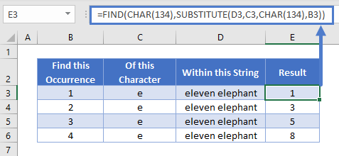
- Finding the nth Character in a String
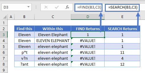
- FIND Vs SEARCH
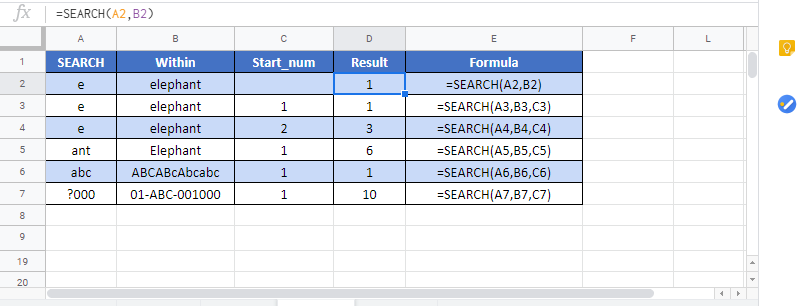
- FIND in Google Sheets
- Additional Notes
- FIND Examples in VBA
- Excel ISNUMBER function with formula examples
- Excel ISNUMBER function
- 2 things you should know about ISNUMBER function in Excel
- Excel ISNUMBER formula examples
- Check if a value is number
- Excel ISNUMBER SEARCH formula
- ISNUMBER FIND — case-sensitive formula
- How this formula works
- IF ISNUMBER formula
- Example 1. Cell contains which text
- Example 2. First character in a cell is number or text
- Check if a value is not number
- Check if a range contains any number
- How this formula works
- ISNUMBER in conditional formatting to highlight cells that contain certain text
Функция НАЙТИ в Excel. Как использовать?
Функция НАЙТИ (FIND) в Excel используется для поиска текстового значения внутри строчки с текстом и указать порядковый номер буквы с которого начинается искомое слово в найденной строке.
Что возвращает функция
Возвращает числовое значение, обозначающее стартовую позицию текстовой строчки внутри другой текстовой строчки.
Синтаксис
=FIND(find_text, within_text, [start_num]) — английская версия
=НАЙТИ(искомый_текст;просматриваемый_текст;[нач_позиция]) — русская версия
Аргументы функции
- find_text (искомый_текст) — текст или строка которую вы хотите найти в рамках другой строки;
- within_text (просматриваемый_текст) — текст, внутри которого вы хотите найти аргумент find_text (искомый_текст);
- [start_num] ([нач_позиция]) — число, отображающее позицию, с которой вы хотите начать поиск. Если аргумент не указать, то поиск начнется сначала.
Дополнительная информация
- Если стартовое число не указано, то функция начинает поиск искомого текста с начала строки;
- Функция НАЙТИ чувствительна к регистру. Если вы хотите сделать поиск без учета регистра, используйте функцию SEARCH в Excel;
- Функция не учитывает подстановочные знаки при поиске. Если вы хотите использовать подстановочные знаки для поиска, используйте функцию SEARCH в Excel;
- Функция каждый раз возвращает ошибку, когда не находит искомый текст в заданной строке.
Примеры использования функции НАЙТИ в Excel
Пример 1. Ищем слово в текстовой строке (с начала строки)
![]()
На примере выше мы ищем слово «Доброе» в словосочетании «Доброе Утро». По результатам поиска, функция выдает число «1», которое обозначает, что слово «Доброе» начинается с первой по очереди буквы в, заданной в качестве области поиска, текстовой строке.
Обратите внимание, что так как функция НАЙТИ в Excel чувствительна к регистру, вы не сможете найти слово «доброе» в словосочетании «Доброе утро», так как оно написано с маленькой буквы. Для того, чтобы осуществить поиска без учета регистра следует пользоваться функцией SEARCH .
Пример 2. Ищем слово в текстовой строке (с заданным порядковым номером старта поиска)
![]()
Третий аргумент функции НАЙТИ указывает позицию, с которой функция начинает поиск искомого значения. На примере выше функция возвращает число «1» когда мы начинаем поиск слова «Доброе» в словосочетании «Доброе утро» с начала текстовой строки. Но если мы зададим аргумент функции start_num (нач_позиция) со значением «2», то функция выдаст ошибку, так как начиная поиск со второй буквы текстовой строки, она не может ничего найти.
Если вы не укажете номер позиции, с которой функции следует начинать поиск искомого аргумента, то Excel по умолчанию начнет поиск с самого начала текстовой строки.
Пример 3. Поиск текстового значения внутри текстовой строки с дублированным искомым значением
![]()
На примере выше мы ищем слово «Доброе» в словосочетании «Доброе Доброе утро». Когда мы начинаем поиск слова «Доброе» с начала текстовой строки, то функция выдает число «1», так как первое слово «Доброе» начинается с первой буквы в словосочетании «Доброе Доброе утро».
Но, если мы укажем в качестве аргумента start_num (нач_позиция) число «2» и попросим функцию начать поиск со второй буквы в заданной текстовой строке, то функция выдаст число «6», так как Excel находит искомое слово «Доброе» начиная со второй буквы словосочетания «Доброе Доброе утро» только на 6 позиции.
Источник
FIND Function Examples In Excel, VBA, & Google Sheets
Download the example workbook
This tutorial demonstrates how to use the FIND Function in Excel and Google Sheets to find text within text.
What Is the FIND Function?
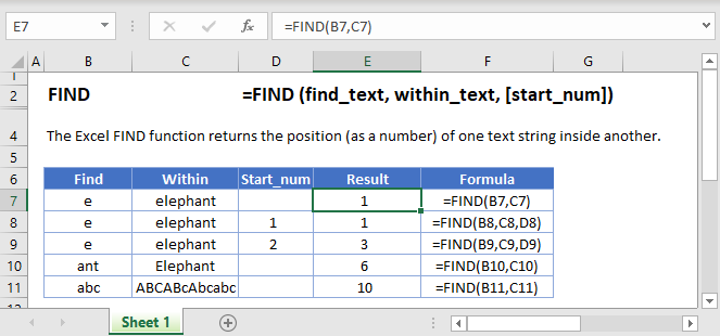
The Excel FIND Function tries to find string of text within another text string. If it finds it, FIND returns the numerical position of that string.
Note: FIND is case-sensitive. So, “text” will NOT match “TEXT”. For case-insensitive searches, use the SEARCH Function.
How to Use the FIND Function
To use the Excel FIND Function, type the following:
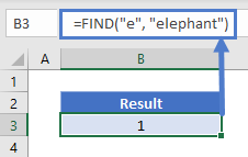
In this case, Excel will return the number 1, because “e” is the first character in the string “elephant”.
Let’s take a look at some more examples:
Start Number (start_num)
The start number tells FIND what numerical position in the string to start looking from. If you don’t define it, FIND will start from the beginning of the string.
Now let’s try defining a start number of 2. Here, we see that FIND returns 3. Because it starts looking from the second character, it misses the first “e” and finds the second:
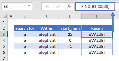
Start Number (start_num) Errors
If you want to use a start number, it must:
- be a whole number
- be a positive number
- be smaller than the length of the string you are looking in
- not refer to a blank cell, if you define it as a cell reference
Otherwise, FIND will return a #VALUE! error as shown below:
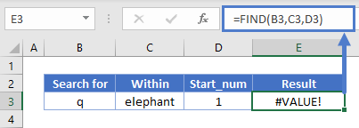
Unsuccessful Searches Return a #VALUE! Error
If FIND does not locate the string you’re looking for, it will return a value error:
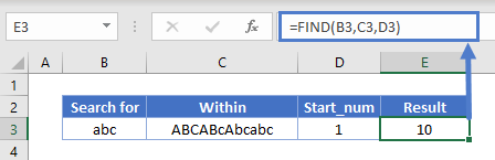
FIND is Case-Sensitive
In the example below, we’re searching for “abc”. FIND returns 10 because it is case-sensitive – it ignores “ABC” and the other variations:
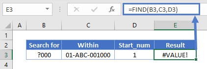
FIND Does Not Accept Wildcards
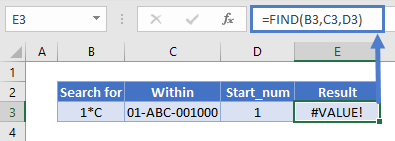
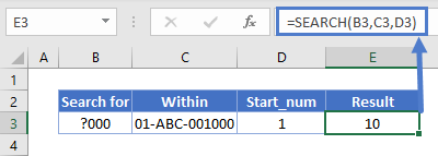
You cannot use wildcards with FIND. Below, we’re looking for “?000”. In a wildcard search, this would mean “any character followed by three zeroes”. But FIND takes this literally to mean “a question mark followed by three zeroes”:
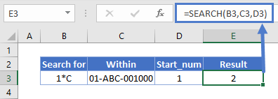
The same applies to the asterisk wildcard:
Instead, to search text with wildcards, you can use the SEARCH Function:
How to Split First and Last Names from a Cell with FIND
If your spreadsheet has a list of names with both the first and last names in the same cell, you might want to split them out to make sorting easier. FIND can do that for you – with a little help from some other functions.
Getting the First Name
The LEFT Function returns a given number of characters from a string, starting from the left.
We can use it to get the first name, but since names are different lengths, how do we know how many characters to return?
Easy – we just use FIND to return the position of the space between the first and last name, subtract 1 from that, and that’s how many characters we tell LEFT to give us.
The formula looks like this:
Getting the Last Name
The RIGHT Function returns a given number of characters from a string, starting from the right.
We have the same problem here as with the first name, but the solution is different, because we have to get the number of characters between the space and the right edge of the string, not the left.
To get that, we use FIND to tell us where the space is, and then subtract that number from the total number of characters in the string, which the LEN Function can give us.
The formula looks like this:
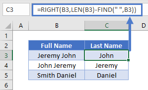
If the name contains a middle name, note that it will be split into the last name cell.
Finding the nth Character in a String
As noted above, FIND returns the position of the first match it finds. But what if you want to find the second occurrence of a particular character, or the third, or fourth?
This is possible with FIND, but we’ll need to combine it with a couple of other functions: CHAR and SUBSTITUTE.
Here’s how it works:
- CHAR returns a character based on its ASCII code. For example, =CHAR(134) returns the dagger symbol.
- SUBSTITUTE goes through a string and lets you swap out a character for any other one.
- With SUBSTITUTE you can define an instance number, meaning it can swap the nth occurrence of a given string for anything else.
- So, the idea is, we take our string, use SUBSTITUTE to swap the instance of the character we want to find for something else. We’ll use CHAR to swap it for something that is unlikely to be found in the string, then use FIND to locate that obscure substitute.
The formula looks like this:
And here’s how it works in practice:
FIND Vs SEARCH
FIND and SEARCH are very similar – they both return the position of a given character or substring within a string. However, there are some differences:
- FIND is case sensitive but SEARCH is not
- FIND does not allow wildcards, but SEARCH does
You can see a few examples of these differences below:
FIND in Google Sheets
The FIND Function works exactly the same in Google Sheets as in Excel:
Additional Notes
The FIND Function is case-sensitive.
The FIND Function does not support wildcards.
Use the SEARCH Function to use wildcards and for non case-sensitive searches.
FIND Examples in VBA
You can also use the FIND function in VBA. Type:
For the function arguments (find_text, etc.), you can either enter them directly into the function, or define variables to use instead.
Источник
Excel ISNUMBER function with formula examples
 by Svetlana Cheusheva, updated on March 14, 2023
The tutorial explains what ISNUMBER in Excel is and provides examples of basic and advanced uses.
The concept of the ISNUMBER function in Excel is very simple — it just checks whether a given value is a number or not. An important point here is that the practical uses of the function go far beyond its basic concept, especially when combined with other functions within larger formulas.
Excel ISNUMBER function
The ISNUMBER function in Excel checks if a cell contains a numerical value or not. It belongs to the group of IS functions.
The function is available in all versions of Excel for Office 365, Excel 2019, Excel 2016, Excel 2013, Excel 2010, Excel 2007 and lower.
The ISNUMBER syntax requires just one argument:
Where value is the value you want to test. Usually, it is represented by a cell reference, but you can also supply a real value or nest another function inside ISNUMBER to check the result.
If value is numeric, the function returns TRUE. For anything else (text values, errors, blanks) ISNUMBER returns FALSE.
As an example, let’s test values in cells A2 through A6, and we will find out that the first 3 values are numbers and the last two are text: 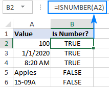
2 things you should know about ISNUMBER function in Excel
There are a couple of interesting points to note here:
- In internal Excel representation, dates and times are numeric values, so the ISNUMBER formula returns TRUE for them (please see B3 and B4 in the screenshot above).
- For numbers stored as text, the ISNUMBER function returns FALSE (see this example).
Excel ISNUMBER formula examples
The below examples demonstrate a few common and a couple of non-trivial uses of ISNUMBER in Excel.
Check if a value is number
When you have a bunch of values in your worksheet and you want to know which ones are numbers, ISNUMBER is the right function to use.
In this example, the first value is in A2, so we use the below formula to check it, and then drag down the formula to as many cells as needed:
=ISNUMBER(A2) 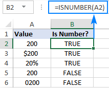
Please pay attention that although all the values look like numbers, the ISNUMBER formula has returned FALSE for cells A4 and A5, which means those values are numeric strings, i.e. numbers formatted as text. There may be different reasons for this, for example leading zeros, preceding apostrophe, etc. Whatever the reason, Excel does not recognize such values as numbers. So, if your values do not calculate correctly, the first thing for you to check is whether they are really numbers in terms of Excel, and then convert text to number if needed.
Excel ISNUMBER SEARCH formula
Apart from identifying numbers, the Excel ISNUMBER function can also check if a cell contains specific text as part of the content. For this, use ISNUMBER together with the SEARCH function.
In the generic form, the formula looks as follows:
Where substring is the text that you want to find.
As an example, let’s check whether the string in A3 contains a specific color, say red:
This formula works nicely for a single cell. But because our sample table (please see below) contains three different colors, writing a separate formula for each one would be the waste of time. Instead, we will refer to the cell containing the color of interest (B2).
For the formula to correctly copy down and to the right, be sure to lock the following coordinates with the $ sign:
- In substring reference, lock the row (B$2) so that the copied formulas always pick the substrings in row 2. The column reference is relative because we want it to adjust for each column, i.e. when the formula is copied to C3, the substring reference will change to C$2.
- In the source cell reference, lock the column ($A3) so that all the formulas check the values in column A.
The screenshot below shows the result: 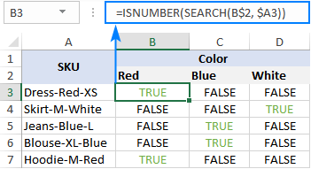
ISNUMBER FIND — case-sensitive formula
As the SEARCH function is case-insensitive, the above formula does not differentiate uppercase and lowercase characters. If you are looking for a case-sensitive formula, use the FIND function rather than SEARCH.
For our sample dataset, the formula would take this form:
How this formula works
The formula’s logic is quite obvious and easy to follow:
- The SEARCH / FIND function looks for the substring in the specified cell. If the substring is found, the position of the first character is returned. If the substring is not found, the function produces a #VALUE! error.
- The ISNUMBER function takes it from there and processes numeric positions. So, if the substring is found and its position is returned as a number, ISNUMBER outputs TRUE. If the substring is not found and a #VALUE! error occurs, ISNUMBER outputs FALSE.
IF ISNUMBER formula
If you aim to get a formula that outputs something other than TRUE or FALSE, use ISNUMBER together with the IF function.
Example 1. Cell contains which text
Taking the previous example further, suppose you want to mark the color of each item with «x» like shown in the table below.
To have this done, simply wrap the ISNUMBER SEARCH formula into the IF statement:
=IF(ISNUMBER(SEARCH(B$2, $A3)), «x», «»)
If ISNUMBER returns TRUE, the IF function outputs «x» (or any other value you supply to the value_if_true argument). If ISNUMBER returns FALSE, the IF function outputs an empty string («»). 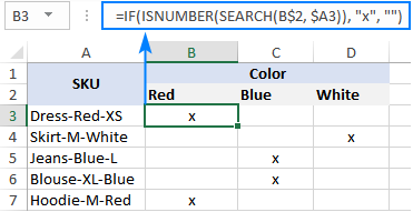
Example 2. First character in a cell is number or text
Imagine that you are working with a list of alphanumeric strings and you want to know whether a string’s first character is a number or letter.
To build such a formula, we you’ll need 4 different functions:
- The LEFT function extracts the first character from the start of a string, say in cell A2:
LEFT(A2, 1)
Because LEFT belongs to the category of Text functions, its result is always a text string, even if it only contains numbers. Therefore, before checking the extracted character, we need to try to convert it to a number. For this, use either the VALUE function or double unary operator:
VALUE(LEFT(A2, 1)) or (—LEFT(A2, 1))
The ISNUMBER function determines if the extracted character is numeric or not:
ISNUMBER(VALUE(LEFT(A2, 1)))
Assuming we are testing a string in A2, the complete formula takes this shape:
=IF(ISNUMBER(VALUE(LEFT(A2, 1))), «Number», «Letter»)
=IF(ISNUMBER(—LEFT(A2, 1)), «Number», «Letter») 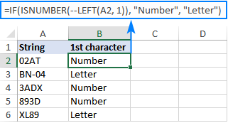
The ISNUMBER function also comes in handy for extracting numbers from a string. Here’s an example: Get number from any position in a string.
Check if a value is not number
Though Microsoft Excel has a special function, ISNONTEXT, to determine whether a cell’s value is not text, an analogous function for numbers is missing.
An easy solution is to use ISNUMBER in combination with NOT that returns the opposite of a logical value. In other words, when ISNUMBER returns TRUE, NOT converts it to FALSE, and the other way round.
To see it in action, please observe the results of the following formula:
=NOT(ISNUMBER(A2)) 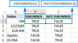
Another approach is using the IF and ISNUMBER functions together:
=IF(ISNUMBER(A2), «», «Not number»)
If A2 is numeric, the formula returns nothing (an empty string). If A2 is not numeric, the formula says it upfront: «Not number». 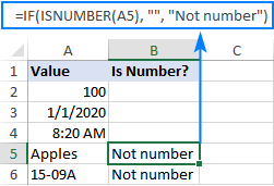
If you’d like to perform some calculations with numbers, then put an equation or another formula in the value_if_true argument instead of an empty string. For example, the below formula will multiply numbers by 10 and yield «Not number» for non-numeric values:
=IF(ISNUMBER(A2), A2*10, «Not number»)
Check if a range contains any number
In situation when you want to test the whole range for numbers, use the ISNUMBER function in combination with SUMPRODUCT like this:
For example, to find out if the range A2:A5 contains any numeric value, the formulas would go as follows:
=SUMPRODUCT(ISNUMBER(A2:A5)*1)>0 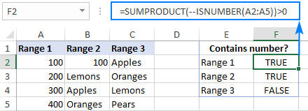
If you’d like to output «Yes» and «No» instead of TRUE and FALSE, utilize the IF statement as a «wrapper» for the above formulas. For example:
=IF(SUMPRODUCT(—ISNUMBER(A2:A5))>0, «Yes», «No») 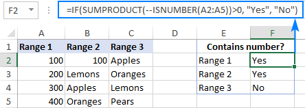
How this formula works
At the heart of the formula, the ISNUMBER function evaluates each cell of the specified range, say B2:B5, and returns TRUE for numbers, FALSE for anything else. As the range contains 4 cells, the array has 4 elements:
The multiplication operation or the double unary (—) coerces TRUE and FALSE into 1’s and 0’s, respectively:
The SUMPRODUCT function adds up the elements of the array. If the result is greater than zero, that means there is at least one number the range. So, you use «>0» to get a final result of TRUE or FALSE.
ISNUMBER in conditional formatting to highlight cells that contain certain text
If you are looking to highlight cells or entire rows that contain specific text, create a conditional formatting rule based on the ISNUMBER SEARCH (case-insensitive) or ISNUMBER FIND (case-sensitive) formula.
For this example, we are going to highlight rows based on the value in column A. More precisely, we will highlight the items that contain the word «red». Here’s how:
- Select all the data rows (A2:C6 in this example) or only the column in which you want to highlight cells.
- On the Home tab, in the Styles group, click New Rule >Use a formula to determine which cells to format.
- In the Format values where this formula is true box, enter the below formula (please notice that the column coordinate is locked with the $ sign):
=ISNUMBER(SEARCH(«red», $A2))
If you have little experience with Excel conditional formatting, you can find the detailed steps with screenshots in this tutorial: How to create a formula-based conditional formatting rule.
As the result, all the items of the red color are highlighted: 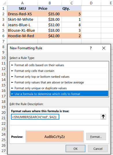
Instead of «hardcoding» the color in the conditional formatting rule, you can type it in a predefined cell, say E2, and refer to that cell in your formula (please mind the absolute cell reference $E$2). Additionally, you need to check if the input cell is not empty:
=AND(ISNUMBER(SEARCH($E$2, $A2)), $E$2<>«»)
As the result, you will get a more flexible rule that highlights rows based on your input in E2: 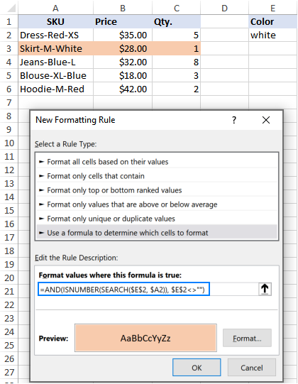
That’s how to use the ISNUMBER function in Excel. I thank you for reading and hope to see you on our blog next week!
Источник
Метод Find объекта Range для поиска ячейки по ее данным в VBA Excel. Синтаксис и компоненты. Знаки подстановки для поисковой фразы. Простые примеры.
Метод Find объекта Range предназначен для поиска ячейки и сведений о ней в заданном диапазоне по ее значению, формуле и примечанию. Чаще всего этот метод используется для поиска в таблице ячейки по слову, части слова или фразе, входящей в ее значение.
Синтаксис метода Range.Find
|
Expression.Find(What, After, LookIn, LookAt, SearchOrder, SearchDirection, MatchCase, MatchByte, SearchFormat) |
Expression – это переменная или выражение, возвращающее объект Range, в котором будет осуществляться поиск.
В скобках перечислены параметры метода, среди них только What является обязательным.
Метод Range.Find возвращает объект Range, представляющий из себя первую ячейку, в которой найдена поисковая фраза (параметр What). Если совпадение не найдено, возвращается значение Nothing.
Если необходимо найти следующие ячейки, содержащие поисковую фразу, используется метод Range.FindNext.
Параметры метода Range.Find
| Наименование | Описание |
|---|---|
| Обязательный параметр | |
| What | Данные для поиска, которые могут быть представлены строкой или другим типом данных Excel. Тип данных параметра — Variant. |
| Необязательные параметры | |
| After | Ячейка, после которой следует начать поиск. |
| LookIn | Уточняет область поиска. Список констант xlFindLookIn:
|
| LookAt | Поиск частичного или полного совпадения. Список констант xlLookAt:
|
| SearchOrder | Определяет способ поиска. Список констант xlSearchOrder:
|
| SearchDirection | Определяет направление поиска. Список констант xlSearchDirection:
|
| MatchCase | Определяет учет регистра:
|
| MatchByte | Условия поиска при использовании двухбайтовых кодировок:
|
| SearchFormat | Формат поиска – используется вместе со свойством Application.FindFormat. |
* Примечания имеют две константы с одним значением. Проверяется очень просто: MsgBox xlComments и MsgBox xlNotes.
В справке Microsoft тип данных всех параметров, кроме SearchDirection, указан как Variant.
Знаки подстановки для поисковой фразы
Условные знаки в шаблоне поисковой фразы:
- ? – знак вопроса обозначает любой отдельный символ;
- * – звездочка обозначает любое количество любых символов, в том числе ноль символов;
- ~ – тильда ставится перед ?, * и ~, чтобы они обозначали сами себя (например, чтобы тильда в шаблоне обозначала сама себя, записать ее нужно дважды: ~~).
Простые примеры
При использовании метода Range.Find в VBA Excel необходимо учитывать следующие нюансы:
- Так как этот метод возвращает объект Range (в виде одной ячейки), присвоить его можно только объектной переменной, объявленной как Variant, Object или Range, при помощи оператора Set.
- Если поисковая фраза в заданном диапазоне найдена не будет, метод Range.Find возвратит значение Nothing. Обращение к свойствам несуществующей ячейки будет генерировать ошибки. Поэтому, перед использованием результатов поиска, необходимо проверить объектную переменную на содержание в ней значения Nothing.
В примерах используются переменные:
- myPhrase – переменная для записи поисковой фразы;
- myCell – переменная, которой присваивается первая найденная ячейка, содержащая поисковую фразу, или значение Nothing, если поисковая фраза не найдена.
Пример 1
|
Sub primer1() Dim myPhrase As Variant, myCell As Range myPhrase = «стакан» Set myCell = Range(«A1:L30»).Find(myPhrase) If Not myCell Is Nothing Then MsgBox «Значение найденной ячейки: « & myCell MsgBox «Строка найденной ячейки: « & myCell.Row MsgBox «Столбец найденной ячейки: « & myCell.Column MsgBox «Адрес найденной ячейки: « & myCell.Address Else MsgBox «Искомая фраза не найдена» End If End Sub |
В этом примере мы присваиваем переменной myPhrase значение для поиска – "стакан". Затем проводим поиск этой фразы в диапазоне "A1:L30" с присвоением результата поиска переменной myCell. Далее проверяем переменную myCell, не содержит ли она значение Nothing, и выводим соответствующие сообщения.
Ознакомьтесь с работой кода VBA в случаях, когда в диапазоне "A1:L30" есть ячейка со строкой, содержащей подстроку "стакан", и когда такой ячейки нет.
Пример 2
Теперь посмотрим, как метод Range.Find отреагирует на поиск числа. В качестве диапазона поиска будем использовать первую строку активного листа Excel.
|
Sub primer2() Dim myPhrase As Variant, myCell As Range myPhrase = 526.15 Set myCell = Rows(1).Find(myPhrase) If Not myCell Is Nothing Then MsgBox «Значение найденной ячейки: « & myCell Else: MsgBox «Искомая фраза не найдена» End If End Sub |
Несмотря на то, что мы присвоили переменной числовое значение, метод Range.Find найдет ячейку со значением и 526,15, и 129526,15, и 526,15254. То есть, как и в предыдущем примере, поиск идет по подстроке.
Чтобы найти ячейку с точным соответствием значения поисковой фразе, используйте константу xlWhole параметра LookAt:
|
Set myCell = Rows(1).Find(myPhrase, , , xlWhole) |
Аналогично используются и другие необязательные параметры. Количество «лишних» запятых перед необязательным параметром должно соответствовать количеству пропущенных компонентов, предусмотренных синтаксисом метода Range.Find, кроме случаев указания необязательного параметра по имени, например: LookIn:=xlValues. Тогда используется одна запятая, независимо от того, сколько компонентов пропущено.
Пример 3
Допустим, у нас есть многострочная база данных в Excel. В первой колонке находятся даты. Нам необходимо создать отчет за какой-то период. Найти номер начальной строки для обработки можно с помощью следующего кода:
|
Sub primer3() Dim myPhrase As Variant, myCell As Range myPhrase = «01.02.2019» myPhrase = CDate(myPhrase) Set myCell = Range(«A:A»).Find(myPhrase) If Not myCell Is Nothing Then MsgBox «Номер начальной строки: « & myCell.Row Else: MsgBox «Даты « & myPhrase & » в таблице нет» End If End Sub |
Несмотря на то, что в ячейке дата отображается в виде текста, ее значение хранится в ячейке в виде числа. Поэтому текстовый формат необходимо перед поиском преобразовать в формат даты.
This tutorial demonstrates how to use the FIND Function in Excel and Google Sheets to find text within text.
What Is the FIND Function?
The Excel FIND Function tries to find string of text within another text string. If it finds it, FIND returns the numerical position of that string.
Note: FIND is case-sensitive. So, “text” will NOT match “TEXT”. For case-insensitive searches, use the SEARCH Function.
How to Use the FIND Function
To use the Excel FIND Function, type the following:
=FIND("e", "elephant")
In this case, Excel will return the number 1, because “e” is the first character in the string “elephant”.
Let’s take a look at some more examples:
Start Number (start_num)
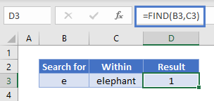
The start number tells FIND what numerical position in the string to start looking from. If you don’t define it, FIND will start from the beginning of the string.
=FIND(B3,C3)
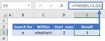
Now let’s try defining a start number of 2. Here, we see that FIND returns 3. Because it starts looking from the second character, it misses the first “e” and finds the second:
=FIND(B3,C3,D3)
Start Number (start_num) Errors
If you want to use a start number, it must:
- be a whole number
- be a positive number
- be smaller than the length of the string you are looking in
- not refer to a blank cell, if you define it as a cell reference
Otherwise, FIND will return a #VALUE! error as shown below:
Unsuccessful Searches Return a #VALUE! Error
If FIND does not locate the string you’re looking for, it will return a value error:
FIND is Case-Sensitive
In the example below, we’re searching for “abc”. FIND returns 10 because it is case-sensitive – it ignores “ABC” and the other variations:
FIND Does Not Accept Wildcards
You cannot use wildcards with FIND. Below, we’re looking for “?000”. In a wildcard search, this would mean “any character followed by three zeroes”. But FIND takes this literally to mean “a question mark followed by three zeroes”:
The same applies to the asterisk wildcard:
Instead, to search text with wildcards, you can use the SEARCH Function:
How to Split First and Last Names from a Cell with FIND
If your spreadsheet has a list of names with both the first and last names in the same cell, you might want to split them out to make sorting easier. FIND can do that for you – with a little help from some other functions.
Getting the First Name
The LEFT Function returns a given number of characters from a string, starting from the left.
We can use it to get the first name, but since names are different lengths, how do we know how many characters to return?
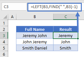
Easy – we just use FIND to return the position of the space between the first and last name, subtract 1 from that, and that’s how many characters we tell LEFT to give us.
The formula looks like this:
=LEFT(B3,FIND(“ “,B3)-1)
Getting the Last Name
The RIGHT Function returns a given number of characters from a string, starting from the right.
We have the same problem here as with the first name, but the solution is different, because we have to get the number of characters between the space and the right edge of the string, not the left.
To get that, we use FIND to tell us where the space is, and then subtract that number from the total number of characters in the string, which the LEN Function can give us.
The formula looks like this:
=RIGHT(B3,LEN(B3)-FIND(" ",B3))
If the name contains a middle name, note that it will be split into the last name cell.
Finding the nth Character in a String
As noted above, FIND returns the position of the first match it finds. But what if you want to find the second occurrence of a particular character, or the third, or fourth?
This is possible with FIND, but we’ll need to combine it with a couple of other functions: CHAR and SUBSTITUTE.
Here’s how it works:
- CHAR returns a character based on its ASCII code. For example, =CHAR(134) returns the dagger symbol.
- SUBSTITUTE goes through a string and lets you swap out a character for any other one.
- With SUBSTITUTE you can define an instance number, meaning it can swap the nth occurrence of a given string for anything else.
- So, the idea is, we take our string, use SUBSTITUTE to swap the instance of the character we want to find for something else. We’ll use CHAR to swap it for something that is unlikely to be found in the string, then use FIND to locate that obscure substitute.
The formula looks like this:
=FIND(CHAR(134),SUBSTITUTE(D3,C3,CHAR(134),B3))And here’s how it works in practice:
FIND Vs SEARCH
FIND and SEARCH are very similar – they both return the position of a given character or substring within a string. However, there are some differences:
- FIND is case sensitive but SEARCH is not
- FIND does not allow wildcards, but SEARCH does
You can see a few examples of these differences below:
FIND in Google Sheets
The FIND Function works exactly the same in Google Sheets as in Excel:
Additional Notes
The FIND Function is case-sensitive.
The FIND Function does not support wildcards.
Use the SEARCH Function to use wildcards and for non case-sensitive searches.
FIND Examples in VBA
You can also use the FIND function in VBA. Type:
application.worksheetfunction.find(find_text,within_text,start_num)For the function arguments (find_text, etc.), you can either enter them directly into the function, or define variables to use instead.
Purpose
Get location substring in a string
Return value
A number representing the location of substring
Usage notes
The FIND function returns the position (as a number) of one text string inside another. If there is more than one occurrence of the search string, FIND returns the position of the first occurrence. When the text is not found, FIND returns a #VALUE error. Also note, when find_text is empty, FIND returns 1. FIND does not support wildcards, and is always case-sensitive. Use the SEARCH function to find the position of text without case-sensitivity and with wildcard support.
Basic Example
The FIND function is designed to look inside a text string for a specific substring. When FIND locates the substring, it returns a position of the substring in the text as a number. If the substring is not found, FIND returns a #VALUE error. For example:
=FIND("p","apple") // returns 2
=FIND("z","apple") // returns #VALUE!
Note that text values entered directly into FIND must be enclosed in double-quotes («»).
Case-sensitive
The FIND function always case-sensitive:
=FIND("a","Apple") // returns #VALUE!
=FIND("A","Apple") // returns 1
TRUE or FALSE result
To force a TRUE or FALSE result, nest the FIND function inside the ISNUMBER function. ISNUMBER returns TRUE for numeric values and FALSE for anything else. If FIND locates the substring, it returns the position as a number, and ISNUMBER returns TRUE:
=ISNUMBER(FIND("p","apple")) // returns TRUE
=ISNUMBER(FIND("z","apple")) // returns FALSE
If FIND doesn’t locate the substring, it returns an error, and ISNUMBER returns FALSE.
Start number
The FIND function has an optional argument called start_num, that controls where FIND should begin looking for a substring. To find the first match of «the» in any combination of upper or lowercase, you can omit start_num, which defaults to 1:
=FIND("x","20 x 30 x 50") // returns 4To start searching at character 5, enter 4 for start_num:
=FIND("x","20 x 30 x 50",5) // returns 9
Wildcards
The FIND function does not support wildcards. See the SEARCH function.
If cell contains
To return a custom result with the SEARCH function, use the IF function like this:
=IF(ISNUMBER(FIND(substring,A1)), "Yes", "No")
Instead of returning TRUE or FALSE, the formula above will return «Yes» if substring is found and «No» if not.
Notes
- The FIND function returns the location of the first find_text in within_text.
- The location is returned as the number of characters from the start.
- Start_num is optional and defaults to 1.
- FIND returns 1 when find_text is empty.
- FIND returns #VALUE if find_text is not found.
- FIND is case-sensitive but does not support wildcards.
- Use the SEARCH function to find a substring with wildcards.
Excel for Microsoft 365 Excel for Microsoft 365 for Mac Excel for the web Excel 2021 Excel 2021 for Mac Excel 2019 Excel 2019 for Mac Excel 2016 Excel 2016 for Mac Excel 2013 Excel 2010 Excel 2007 Excel for Mac 2011 Excel Starter 2010 More…Less
This article describes the formula syntax and usage of the FIND and FINDB functions in Microsoft Excel.
Description
FIND and FINDB locate one text string within a second text string, and return the number of the starting position of the first text string from the first character of the second text string.
Important:
-
These functions may not be available in all languages.
-
FIND is intended for use with languages that use the single-byte character set (SBCS), whereas FINDB is intended for use with languages that use the double-byte character set (DBCS). The default language setting on your computer affects the return value in the following way:
-
FIND always counts each character, whether single-byte or double-byte, as 1, no matter what the default language setting is.
-
FINDB counts each double-byte character as 2 when you have enabled the editing of a language that supports DBCS and then set it as the default language. Otherwise, FINDB counts each character as 1.
The languages that support DBCS include Japanese, Chinese (Simplified), Chinese (Traditional), and Korean.
Syntax
FIND(find_text, within_text, [start_num])
FINDB(find_text, within_text, [start_num])
The FIND and FINDB function syntax has the following arguments:
-
Find_text Required. The text you want to find.
-
Within_text Required. The text containing the text you want to find.
-
Start_num Optional. Specifies the character at which to start the search. The first character in within_text is character number 1. If you omit start_num, it is assumed to be 1.
Remarks
-
FIND and FINDB are case sensitive and don’t allow wildcard characters. If you don’t want to do a case sensitive search or use wildcard characters, you can use SEARCH and SEARCHB.
-
If find_text is «» (empty text), FIND matches the first character in the search string (that is, the character numbered start_num or 1).
-
Find_text cannot contain any wildcard characters.
-
If find_text does not appear in within_text, FIND and FINDB return the #VALUE! error value.
-
If start_num is not greater than zero, FIND and FINDB return the #VALUE! error value.
-
If start_num is greater than the length of within_text, FIND and FINDB return the #VALUE! error value.
-
Use start_num to skip a specified number of characters. Using FIND as an example, suppose you are working with the text string «AYF0093.YoungMensApparel». To find the number of the first «Y» in the descriptive part of the text string, set start_num equal to 8 so that the serial-number portion of the text is not searched. FIND begins with character 8, finds find_text at the next character, and returns the number 9. FIND always returns the number of characters from the start of within_text, counting the characters you skip if start_num is greater than 1.
Examples
Copy the example data in the following table, and paste it in cell A1 of a new Excel worksheet. For formulas to show results, select them, press F2, and then press Enter. If you need to, you can adjust the column widths to see all the data.
|
Data |
||
|
Miriam McGovern |
||
|
Formula |
Description |
Result |
|
=FIND(«M»,A2) |
Position of the first «M» in cell A2 |
1 |
|
=FIND(«m»,A2) |
Position of the first «M» in cell A2 |
6 |
|
=FIND(«M»,A2,3) |
Position of the first «M» in cell A2, starting with the third character |
8 |
Example 2
|
Data |
||
|
Ceramic Insulators #124-TD45-87 |
||
|
Copper Coils #12-671-6772 |
||
|
Variable Resistors #116010 |
||
|
Formula |
Description (Result) |
Result |
|
=MID(A2,1,FIND(» #»,A2,1)-1) |
Extracts text from position 1 to the position of «#» in cell A2 (Ceramic Insulators) |
Ceramic Insulators |
|
=MID(A3,1,FIND(» #»,A3,1)-1) |
Extracts text from position 1 to the position of «#» in cell A3 (Copper Coils) |
Copper Coils |
|
=MID(A4,1,FIND(» #»,A4,1)-1) |
Extracts text from position 1 to the position of «#» in cell A4 (Variable Resistors) |
Variable Resistors |
Need more help?
Want more options?
Explore subscription benefits, browse training courses, learn how to secure your device, and more.
Communities help you ask and answer questions, give feedback, and hear from experts with rich knowledge.