
Excel for Microsoft 365 Excel 2021 Excel 2019 Excel 2016 Excel 2013 Excel 2010 More…Less
Suppose you need to change some formulas in a hurry, but you’re new to the workbook and you don’t know where the formulas are. Here’s how to find them.
-
Select a cell, or a range of cells.
If you select one cell, you search the whole worksheet. If you select a range, you search just that range.
-
Click Home > Find & Select > Go To Special.
-
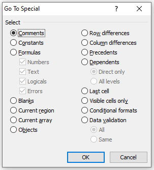
Click Formulas, and if you need to, clear any of the check boxes below Formulas.
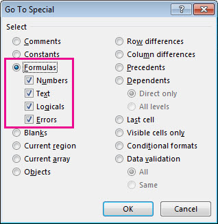
4. Click OK.
More about finding things in Excel
-
Find or replace text and numbers on a worksheet
-
Find merged cells
-
Find ranges by using defined names
-
Remove or allow a circular reference
-
Find hidden cells on a worksheet
Need more help?
Want more options?
Explore subscription benefits, browse training courses, learn how to secure your device, and more.
Communities help you ask and answer questions, give feedback, and hear from experts with rich knowledge.
A few days back I had a huge spreadsheet in which I had to find out the cells containing formulas. Initially, I was totally clueless about how this task can be done.
But later after doing some Google searches, I got a few ideas on how I can effortlessly identify the formula cells in excel.
And today to share my experiences with you guys, In this post I will throw some light on a few methods that can help you to find out formula cells in your spreadsheets.
So here we go:
Method 1: Using ‘Go To Special’ Option:
In Excel ‘Go To Special’ is a very handy option when it comes to finding the cells with formulas. ‘Go to Special’ option has a radio button “Formulas” and selecting this radio button enables it to select all the cells containing formulas.
Later you can change the formatting or background color of the selected cells to make them stand out from the rest. Below is the step by step instructions for accomplishing this:
1. With your excel sheet opened navigate to the ‘Home’ tab > ‘Find & Select’ > ‘Go To Special’. Alternatively, you can also press ‘F5’ and then ‘Alt + S’ to open the ‘Go to Special’ dialog.

2. Next, in the ‘Go to Special’ window select the ‘Formulas’ radio button. After checking this radio button you will notice that few checkboxes (like Numbers, Errors, Logical, and Text) are enabled, these checkboxes signify the return type of the formulas.
So, if you select the ‘Formulas’ radio button and only check the ‘Numbers’ checkbox then it will just search the Formulas whose return type is a number. Here in our example, we will keep all of these return types checked.
3. After this click the ‘Ok’ button and all the cells that contain formulas get selected.
4. Next, without clicking anywhere on your spreadsheet change the background color of all the selected cells.
5. Now your formula cells can be easily identified.
Method 2: Using a built-in Excel formula
If you have worked with excel formulas then probably you may be knowing that excel has a formula that can find whether a cell contains a formula or not. The formula that I am talking about is:
=ISFORMULA(reference)
Here ‘reference’ signifies the cell position which you wish to check for the presence of a formula.
For example: If you wish to check the cell ‘A2’ for the existence of a formula then you can use this function as
=ISFORMULA(A2)
This function results in a Boolean output i.e. True or False. True signifies that the cell contains formulas while False tells that cell doesn’t contain any formulas.
Method 3: Using a Macro for identifying the cells that contain formulas:
I have created a VBA Macro that can find and color any cells that contain the formula in the total used range of the Active sheet. To use this macro simply follow the below procedure:
1. Open your spreadsheet and hit the ‘Alt + F11’ keys to open the VBA editor.

2. Next, navigate to ‘Insert‘ > ‘Module‘ and then paste the below macro in the editor.
Sub FindFormulaCells()
For Each cl In ActiveSheet.UsedRange
If cl.HasFormula() = True Then
cl.Interior.ColorIndex = 24
End If
Next cl
End Sub
3. For running this formula press the “F5” key.
4. This Macro will change the background colour of all the formula containing cells and thus makes it easier to identify them easily.
Recommended Reading: How to add a Checkbox in excel
Содержание
- How to Find Cells containing Formulas in Excel
- Method 1: Using ‘Go To Special’ Option:
- Method 2: Using a built-in Excel formula
- Method 3: Using a Macro for identifying the cells that contain formulas:
- Subscribe and be a part of our 15,000+ member family!
- FIND, FINDB functions
- Description
- Syntax
- Remarks
- Examples
- Use Excel built-in functions to find data in a table or a range of cells
- Summary
- Create the Sample Worksheet
- Term Definitions
- Functions
- LOOKUP()
- VLOOKUP()
- INDEX() and MATCH()
- OFFSET() and MATCH()
- FIND Function
- Related functions
- Summary
- Purpose
- Return value
- Arguments
- Syntax
- Usage notes
- Basic Example
- Case-sensitive
- TRUE or FALSE result
- Start number
- Wildcards
- If cell contains
How to Find Cells containing Formulas in Excel
A few days back I had a huge spreadsheet in which I had to find out the cells containing formulas. Initially, I was totally clueless about how this task can be done.
But later after doing some Google searches, I got a few ideas on how I can effortlessly identify the formula cells in excel.
And today to share my experiences with you guys, In this post I will throw some light on a few methods that can help you to find out formula cells in your spreadsheets.
Method 1: Using ‘Go To Special’ Option:
In Excel ‘Go To Special’ is a very handy option when it comes to finding the cells with formulas. ‘Go to Special’ option has a radio button “Formulas” and selecting this radio button enables it to select all the cells containing formulas.
Later you can change the formatting or background color of the selected cells to make them stand out from the rest. Below is the step by step instructions for accomplishing this:
1. With your excel sheet opened navigate to the ‘Home’ tab > ‘Find & Select’ > ‘Go To Special’. Alternatively, you can also press ‘F5’ and then ‘Alt + S’ to open the ‘Go to Special’ dialog.

2. Next, in the ‘Go to Special’ window select the ‘Formulas’ radio button. After checking this radio button you will notice that few checkboxes (like Numbers, Errors, Logical, and Text) are enabled, these checkboxes signify the return type of the formulas.
So, if you select the ‘Formulas’ radio button and only check the ‘Numbers’ checkbox then it will just search the Formulas whose return type is a number. Here in our example, we will keep all of these return types checked.
3. After this click the ‘Ok’ button and all the cells that contain formulas get selected.
4. Next, without clicking anywhere on your spreadsheet change the background color of all the selected cells.
5. Now your formula cells can be easily identified.
Method 2: Using a built-in Excel formula
If you have worked with excel formulas then probably you may be knowing that excel has a formula that can find whether a cell contains a formula or not. The formula that I am talking about is:
Here ‘reference’ signifies the cell position which you wish to check for the presence of a formula.
For example: If you wish to check the cell ‘A2’ for the existence of a formula then you can use this function as
This function results in a Boolean output i.e. True or False. True signifies that the cell contains formulas while False tells that cell doesn’t contain any formulas.
Method 3: Using a Macro for identifying the cells that contain formulas:
I have created a VBA Macro that can find and color any cells that contain the formula in the total used range of the Active sheet. To use this macro simply follow the below procedure:
1. Open your spreadsheet and hit the ‘Alt + F11’ keys to open the VBA editor.

2. Next, navigate to ‘Insert‘ > ‘Module‘ and then paste the below macro in the editor.
3. For running this formula press the “F5” key.
4. This Macro will change the background colour of all the formula containing cells and thus makes it easier to identify them easily.
Subscribe and be a part of our 15,000+ member family!
Now subscribe to Excel Trick and get a free copy of our ebook «200+ Excel Shortcuts» (printable format) to catapult your productivity.
Источник
FIND, FINDB functions
This article describes the formula syntax and usage of the FIND and FINDB functions in Microsoft Excel.
Description
FIND and FINDB locate one text string within a second text string, and return the number of the starting position of the first text string from the first character of the second text string.
These functions may not be available in all languages.
FIND is intended for use with languages that use the single-byte character set (SBCS), whereas FINDB is intended for use with languages that use the double-byte character set (DBCS). The default language setting on your computer affects the return value in the following way:
FIND always counts each character, whether single-byte or double-byte, as 1, no matter what the default language setting is.
FINDB counts each double-byte character as 2 when you have enabled the editing of a language that supports DBCS and then set it as the default language. Otherwise, FINDB counts each character as 1.
The languages that support DBCS include Japanese, Chinese (Simplified), Chinese (Traditional), and Korean.
Syntax
FIND(find_text, within_text, [start_num])
FINDB(find_text, within_text, [start_num])
The FIND and FINDB function syntax has the following arguments:
Find_text Required. The text you want to find.
Within_text Required. The text containing the text you want to find.
Start_num Optional. Specifies the character at which to start the search. The first character in within_text is character number 1. If you omit start_num, it is assumed to be 1.
FIND and FINDB are case sensitive and don’t allow wildcard characters. If you don’t want to do a case sensitive search or use wildcard characters, you can use SEARCH and SEARCHB.
If find_text is «» (empty text), FIND matches the first character in the search string (that is, the character numbered start_num or 1).
Find_text cannot contain any wildcard characters.
If find_text does not appear in within_text, FIND and FINDB return the #VALUE! error value.
If start_num is not greater than zero, FIND and FINDB return the #VALUE! error value.
If start_num is greater than the length of within_text, FIND and FINDB return the #VALUE! error value.
Use start_num to skip a specified number of characters. Using FIND as an example, suppose you are working with the text string «AYF0093.YoungMensApparel». To find the number of the first «Y» in the descriptive part of the text string, set start_num equal to 8 so that the serial-number portion of the text is not searched. FIND begins with character 8, finds find_text at the next character, and returns the number 9. FIND always returns the number of characters from the start of within_text, counting the characters you skip if start_num is greater than 1.
Examples
Copy the example data in the following table, and paste it in cell A1 of a new Excel worksheet. For formulas to show results, select them, press F2, and then press Enter. If you need to, you can adjust the column widths to see all the data.
Источник
Use Excel built-in functions to find data in a table or a range of cells
Summary
This step-by-step article describes how to find data in a table (or range of cells) by using various built-in functions in Microsoft Excel. You can use different formulas to get the same result.
Create the Sample Worksheet
This article uses a sample worksheet to illustrate Excel built-in functions. Consider the example of referencing a name from column A and returning the age of that person from column C. To create this worksheet, enter the following data into a blank Excel worksheet.
You will type the value that you want to find into cell E2. You can type the formula in any blank cell in the same worksheet.
Term Definitions
This article uses the following terms to describe the Excel built-in functions:
The whole lookup table
The value to be found in the first column of Table_Array.
Lookup_Array
-or-
Lookup_Vector
The range of cells that contains possible lookup values.
The column number in Table_Array the matching value should be returned for.
3 (third column in Table_Array)
Result_Array
-or-
Result_Vector
A range that contains only one row or column. It must be the same size as Lookup_Array or Lookup_Vector.
A logical value (TRUE or FALSE). If TRUE or omitted, an approximate match is returned. If FALSE, it will look for an exact match.
This is the reference from which you want to base the offset. Top_Cell must refer to a cell or range of adjacent cells. Otherwise, OFFSET returns the #VALUE! error value.
This is the number of columns, to the left or right, that you want the upper-left cell of the result to refer to. For example, «5» as the Offset_Col argument specifies that the upper-left cell in the reference is five columns to the right of reference. Offset_Col can be positive (which means to the right of the starting reference) or negative (which means to the left of the starting reference).
Functions
LOOKUP()
The LOOKUP function finds a value in a single row or column and matches it with a value in the same position in a different row or column.
The following is an example of LOOKUP formula syntax:
The following formula finds Mary’s age in the sample worksheet:
The formula uses the value «Mary» in cell E2 and finds «Mary» in the lookup vector (column A). The formula then matches the value in the same row in the result vector (column C). Because «Mary» is in row 4, LOOKUP returns the value from row 4 in column C (22).
NOTE: The LOOKUP function requires that the table be sorted.
For more information about the LOOKUP function, click the following article number to view the article in the Microsoft Knowledge Base:
VLOOKUP()
The VLOOKUP or Vertical Lookup function is used when data is listed in columns. This function searches for a value in the left-most column and matches it with data in a specified column in the same row. You can use VLOOKUP to find data in a sorted or unsorted table. The following example uses a table with unsorted data.
The following is an example of VLOOKUP formula syntax:
The following formula finds Mary’s age in the sample worksheet:
The formula uses the value «Mary» in cell E2 and finds «Mary» in the left-most column (column A). The formula then matches the value in the same row in Column_Index. This example uses «3» as the Column_Index (column C). Because «Mary» is in row 4, VLOOKUP returns the value from row 4 in column C (22).
For more information about the VLOOKUP function, click the following article number to view the article in the Microsoft Knowledge Base:
INDEX() and MATCH()
You can use the INDEX and MATCH functions together to get the same results as using LOOKUP or VLOOKUP.
The following is an example of the syntax that combines INDEX and MATCH to produce the same results as LOOKUP and VLOOKUP in the previous examples:
The following formula finds Mary’s age in the sample worksheet:
The formula uses the value «Mary» in cell E2 and finds «Mary» in column A. It then matches the value in the same row in column C. Because «Mary» is in row 4, the formula returns the value from row 4 in column C (22).
NOTE: If none of the cells in Lookup_Array match Lookup_Value («Mary»), this formula will return #N/A.
For more information about the INDEX function, click the following article number to view the article in the Microsoft Knowledge Base:
OFFSET() and MATCH()
You can use the OFFSET and MATCH functions together to produce the same results as the functions in the previous example.
The following is an example of syntax that combines OFFSET and MATCH to produce the same results as LOOKUP and VLOOKUP:
This formula finds Mary’s age in the sample worksheet:
The formula uses the value «Mary» in cell E2 and finds «Mary» in column A. The formula then matches the value in the same row but two columns to the right (column C). Because «Mary» is in column A, the formula returns the value in row 4 in column C (22).
For more information about the OFFSET function, click the following article number to view the article in the Microsoft Knowledge Base:
Источник
FIND Function

Summary
The Excel FIND function returns the position (as a number) of one text string inside another. When the text is not found, FIND returns a #VALUE error.
Purpose
Return value
Arguments
- find_text — The substring to find.
- within_text — The text to search within.
- start_num — [optional] The starting position in the text to search. Optional, defaults to 1.
Syntax
Usage notes
The FIND function returns the position (as a number) of one text string inside another. If there is more than one occurrence of the search string, FIND returns the position of the first occurrence. When the text is not found, FIND returns a #VALUE error. Also note, when find_text is empty, FIND returns 1. FIND does not support wildcards, and is always case-sensitive. Use the SEARCH function to find the position of text without case-sensitivity and with wildcard support.
Basic Example
The FIND function is designed to look inside a text string for a specific substring. When FIND locates the substring, it returns a position of the substring in the text as a number. If the substring is not found, FIND returns a #VALUE error. For example:
Note that text values entered directly into FIND must be enclosed in double-quotes («»).
Case-sensitive
The FIND function always case-sensitive:
TRUE or FALSE result
To force a TRUE or FALSE result, nest the FIND function inside the ISNUMBER function. ISNUMBER returns TRUE for numeric values and FALSE for anything else. If FIND locates the substring, it returns the position as a number, and ISNUMBER returns TRUE:
If FIND doesn’t locate the substring, it returns an error, and ISNUMBER returns FALSE.
Start number
The FIND function has an optional argument called start_num, that controls where FIND should begin looking for a substring. To find the first match of «the» in any combination of upper or lowercase, you can omit start_num, which defaults to 1:
To start searching at character 5, enter 4 for start_num:
Wildcards
The FIND function does not support wildcards. See the SEARCH function.
If cell contains
To return a custom result with the SEARCH function, use the IF function like this:
Instead of returning TRUE or FALSE, the formula above will return «Yes» if substring is found and «No» if not.
Источник
Many a time, it may have happened with you that you have a lot many formulas in your excel worksheet and you want to find only those cells that contain formulas. One way is to go to each and every cell one by one and then check if it contains any formula or not. But don’t you think that it is a quite time-consuming and irritating activity? Yes, it is. Indeed, there are many easy ways that you can use to find the cells containing formula at one click. In this blog, we would unlock this technique to find formula cells in Excel. There are multiple ways to achieve it.
As mentioned in the introduction paragraph of this blog, there are mainly three ways to find all the cells that contain formula in it. Let me list those down first.
Table of Contents
- Methods to Find Formula Cells
- Sample Example Data
- Find Formula Cells Using ISFORMULA function in Excel
- Using Conditional Formatting to Find Formula Cells
- Using GoTo Special Functionality
- Using the ISFORMULA function
- Using ‘Conditional Formatting’ Feature
- ‘GoTo Special’ Functionality
Sample Example Data
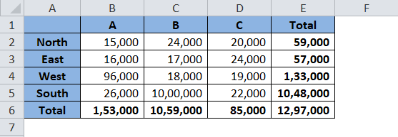
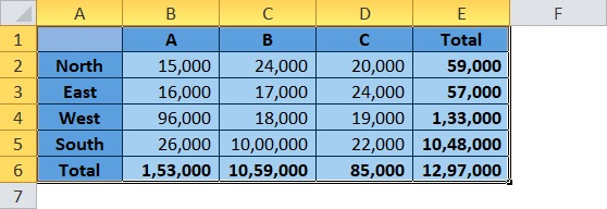
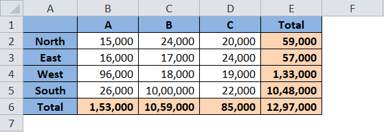
Below is the screenshot of containing sales data in a table format region wise. In this dataset, there are few cells that contain formula in it. The goal here is to find all the cell containing the formula.
Let us now start learning each of the methods one by one.
Find Formula Cells Using ISFORMULA function in Excel
In this method, we would learn how to use an excel pre-provided formula to find all the cells containing a formula in it. The formula about which I am talking about is – ‘ISFORMULA‘.
The formula nomenclature itself makes it clear that this function/formula would check if it IS a FORMULA.
Syntax and Attributes: The formula syntax goes like this: =ISFORMULA(reference); where ‘Reference’ means the reference of the cell or range.
Return Values: This formula returns ‘TRUE‘ if the reference cell contains a formula and ‘FALSE‘ in vice versa situation.
Let us now use this function in our example. Follow the below steps:
Select the exact number of cell range as that of the original data table somewhere in the worksheet. In my example, since I have the data table with 6 rows and 5 columns, therefore, I have selected exactly 6 rows and 5 columns at some other place in Excel (A5:E13). Refer to the screenshot below:
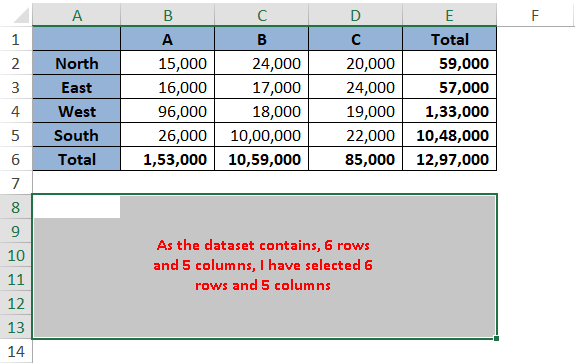
Make sure that the starting cell of the selection should be the top-left cell (in our example it is A8). As can be seen from the screenshot above, we started the selection from cell A8 and therefore, cell A8 is the active cell now.
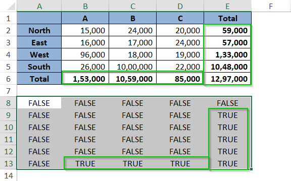
Now, just type the formula =ISFORMULA(A1) and press Ctrl+Enter. As a result, you would notice that Excel enters the same formula in all the cells in the selected cell range.
Consequently, the formula returns TRUE and FALSE as a return value. This depicts that the reference cells corresponding to the cells with TRUE contain a formula. And the reference cells corresponding to the cells with FLASE do not contain any formula.
Using Conditional Formatting to Find Formula Cells
This method is an extension of the above method. One of the limitations of the above method is that the method does not provide the required information (that whether a cell contains a formula) in the cell itself. As you can see, the information that the cell E4 has a formula in it is provided in the cell E11 (as the return value TRUE).
To mitigate this, we can use the conditional formatting functionality along with the ISFORMULA function to find determine a formula cell (in that cell itself). Follow the procedure below:
Firstly, select the cell range (A1 to E6).
Now, navigate to the ‘Home’ tab. There you would find an option called ‘Conditional Formatting’.
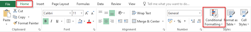
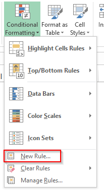
Click on this feature, and select the option ‘New Rule’ from the list of a drop-down menu.
Under the ‘Select a Rule Type’ section, click on the last option ‘Use a formula to determine which cell to format’ and enter the formula =ISFORMULA(A1) in the input box available.
Next, click on the option ‘Format’ to open the ‘Format Cells’ dialog box. Under the tab named ‘Fill’, and select the cell fill color of your choice from the list of available colors (I have selected the Yellow color).
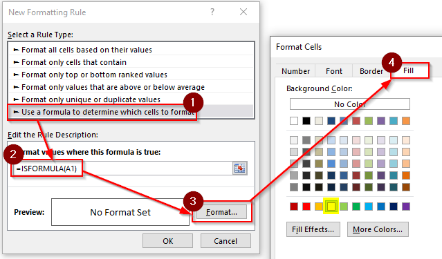
Finally, click on the ‘OK’ button to activate the format cell and then exit the ‘Conditional Formatting’ dialog box by clicking on the ‘OK’ button.
As a result, you would notice that the excel highlights all those cells that have a formula in it.
Using GoTo Special Functionality
This is yet another method to find all the cells containing the formula. This is a widely used method among all the other methods as no formula is needed to use this function. Follow the undermentioned steps-
Firstly, select the dataset table
Now press Ctrl+G key combinations on your keyboard to open the “GoTo” dialog box.
In the “GoTo” dialog box, click on the “Special” option as highlighted in the screenshot below.
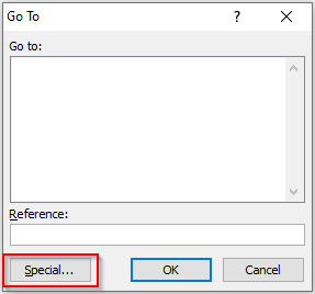
The “GoTo Special” dialog box would open.
From the list of available options, click on the radio button “Formulas” and then click on the “OK” button to exit this dialog box.
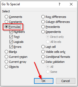
As a result, you would notice that all the formula cells get selected.
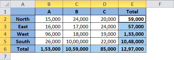
Finally, just change the fill color of all those cells by choosing the color of your choice from the list of available colors. Refer to the screenshot below
You can even do any kind of formatting to these cells, like changing the font size, color, etc.
This brings us to the end of this blog. Share your views and comments in the comment section below.
RELATED POSTS
-
ISNUMBER Function of Excel – Checking If Cell Contains a Number
-
ISNONTEXT Function of Excel – Check Non Text Cell in Excel
-
Using =IF() Function For Partial Match in Excel
-
ISLOGICAL Function in Excel – Checking for Boolean TRUE/FALSE
-
How to Select Cells Containing Data Validation
-
SEARCH Function in Excel – Search String in Excel
In this video, we’re going to look at three ways to find formulas in a worksheet. Knowing where formulas are is the first step in understanding how a spreadsheet works.
When you first open a worksheet you didn’t create yourself, it may not be clear exactly where the formulas are.
Of course, you can just start selecting cells, while watching the formula bar, but there are several faster ways to find all formulas at once.
First, you can toggle the visibility of formulas on or off using the keyboard shortcut Control + Grave Accent. This key is just below the Escape key on US keyboards. This shortcut will cause Excel to display the formulas themselves instead of their results. Using this shortcut, you can quickly and easily switch back and forth.
The next way you can find all formulas is to use Go To Special. Go To Special is based on the Go To Dialog. The fastest way to open this dialog box is to use the keyboard shortcut Control-G. This works on both Windows and Mac platforms.
In the Go To dialog box, click Special, select Formulas, and then click OK. Excel will select all cells that contain formulas.
In the status bar, we can see the number of cells selected.
With all formulas selected, you can easily apply formatting. For example, let’s add a light yellow fill. Now all cells that contain formulas are marked for easy reference.
To clear this formatting. We can just reverse the process.
[go to special, clear formatting]
A third way to visually highlight formulas is to use Conditional Formatting. Excel 2013 includes a new formula called ISFORMULA(), which makes for a very simple Conditional Formatting rule, but that won’t work in older versions of Excel.
Instead, we’ll use a function called GET.CELL(), which is part of the XLM Macro language that preceded VBA. Unfortunately, GET.CELL can’t be used directly in a worksheet. However, by using a named formula, we can work around this problem.
First, we create a new name called CellHasFormula. For the reference, we use the GET.CELL function like so:
=GET.CELL(48,INDIRECT("rc",FALSE))
The first argument—48—tells GET.CELL to return TRUE if a cell contains a formula. The second parameter is the INDIRECT function. In this case, «rc» means current row and column, and FALSE tells INDIRECT that we are using R1C1 style references instead of A1 style references.
Now we can select the range we want to work with and create a new Conditional Formatting rule. We want to use a formula to control formatting, and the formula we use is simply our named formula «CellHasFormula.»
Once we set the format, we’ll see it applied to the cells that contain formulas. Because the highlighting is applied with Conditional Formatting, it’s fully dynamic. If we add a new formula, we’ll see it highlighted too.
One advantage to using Conditional Formatting is that the actual formatting of the cells is not affected. To stop highlighting formulas, simply delete the rule.
The next time you inherit a new workbook, try one of these 3 methods to quickly and easily find all formulas.
Three ways to find and highlight formulas:
1. Toggle Formulas with Control + `
2. Go To Special > Formulas
3. Conditional formatting with GET.CELL as named formula