
Find and remove duplicates
Excel for Microsoft 365 Excel 2021 Excel 2019 Excel 2016 Excel 2013 Excel 2010 Excel 2007 Excel Starter 2010 More…Less
Sometimes duplicate data is useful, sometimes it just makes it harder to understand your data. Use conditional formatting to find and highlight duplicate data. That way you can review the duplicates and decide if you want to remove them.
-
Select the cells you want to check for duplicates.
Note: Excel can’t highlight duplicates in the Values area of a PivotTable report.
-
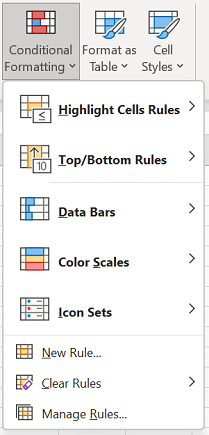
Click Home > Conditional Formatting > Highlight Cells Rules > Duplicate Values.

-
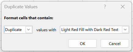
In the box next to values with, pick the formatting you want to apply to the duplicate values, and then click OK.
Remove duplicate values
When you use the Remove Duplicates feature, the duplicate data will be permanently deleted. Before you delete the duplicates, it’s a good idea to copy the original data to another worksheet so you don’t accidentally lose any information.
-
Select the range of cells that has duplicate values you want to remove.
-
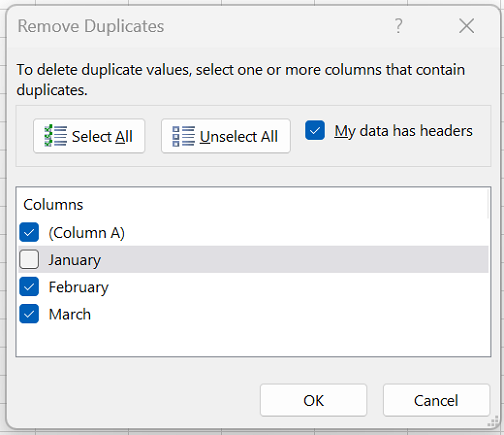
Click Data > Remove Duplicates, and then Under Columns, check or uncheck the columns where you want to remove the duplicates.
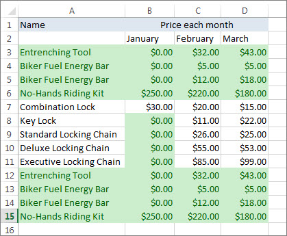
For example, in this worksheet, the January column has price information I want to keep.
So, I unchecked January in the Remove Duplicates box.
-
Click OK.
Note: The counts of duplicate and unique values given after removal may include empty cells, spaces, etc.
Need more help?

Need more help?
Want more options?
Explore subscription benefits, browse training courses, learn how to secure your device, and more.
Communities help you ask and answer questions, give feedback, and hear from experts with rich knowledge.
Note: This tutorial on how to find duplicates in Excel is suitable for Excel 2007, Excel 2010, Excel 2013, Excel 2013, Excel 2019 and Office 365 users.
Duplicate rows of data in a spreadsheet are every Excel user’s cause for a headache. They are annoying to deal with and eat a lot of time while cleaning up.
You might have come across some guides bombarding you with complicated formulas to deal with duplicate rows.
Related:
Excel Goal Seek—the Easiest Guide (3 Examples)
Create A Pivot Table In Excel—the Easiest Guide
Excel Conditional Formatting -the Best Guide (Bonus Video)
Don’t fret. I have created this easy guide on how to find duplicates in Excel, making it a walk in the park for you.
By the end of this guide, you’ll be able to find, highlight, count, filter, and remove duplicates in Excel instantly.
In this article we’ll cover:
- Find Duplicates in Excel Using Conditional Formatting
- How to Highlight Duplicates in Excel?
- How to Find Duplicate Cells with the Exact Number of Occurrences?
- How to Find Duplicate Rows in Excel?
- How to Remove Duplicate Rows in Excel?
- How to Use COUNTIF / COUNTIFS to Find Duplicates in Excel?
- How to Find Duplicates in Excel Using COUNTIF?
- How to Find Case Sensitive Duplicates?
- How to Find Duplicate Rows in Excel Using COUNTIFS?
- How to Count Duplicates in Excel Using COUNTIF?
- How to Count the Number of Duplicate Rows in Excel Using COUNTIFS?
- How to Filter Duplicates in Excel?
Find Duplicates in Excel Using Conditional Formatting
Conditional formatting is one of the quickest ways to find duplicates in Excel. It is a straightforward tool for highlighting duplicate values or duplicate rows in a sheet.
But, it’ll only work properly when you keep some important things in mind. We’ll cover these with the help of the following examples.
How to Highlight Duplicates in Excel?
Let’s look at how to accomplish this with the help of these simple steps.
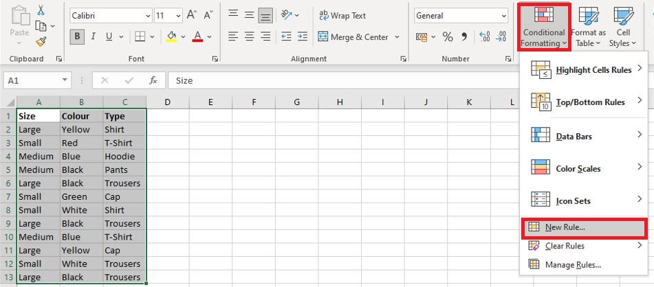
- Get your Data ready as show below. I recommend you create named ranges for your columns, but it is not necessary.
- Select your Data and click on the Conditional Formatting button under the Home Ribbon
- Under Highlight Cell Rules, click on Duplicate Values.
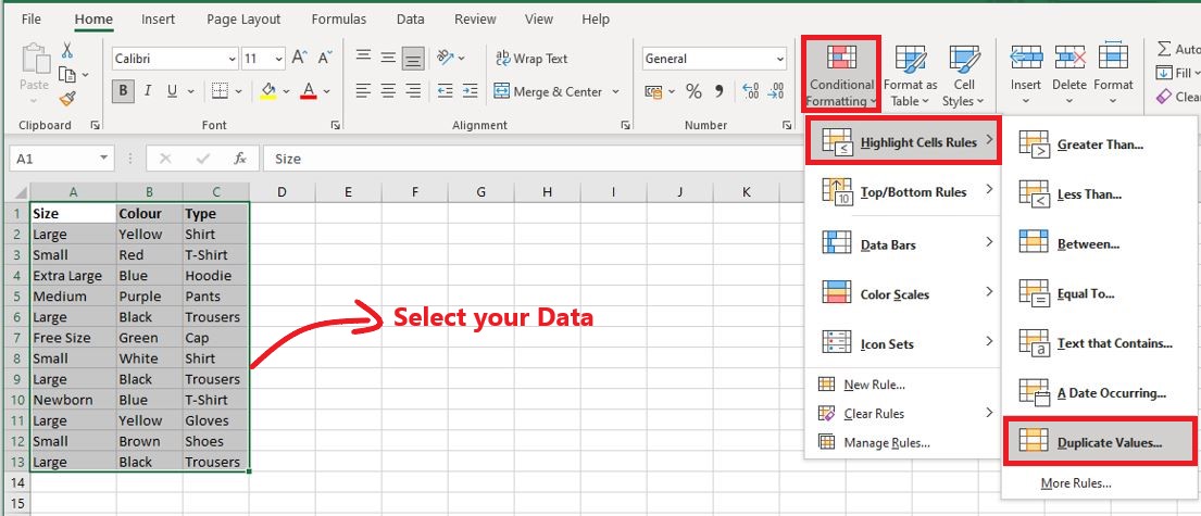
- Choose your preferred Format option or create a custom format.

- Click OK
- You have successfully highlighted duplicates in Excel.
Notice that doing this will highlight all instances of recurrence in the data range.
Also Read:
The Best Excel Project Management Template In 2021
How To Use Excel Countifs: The Best Guide
Excel Sumifs & Sumif Functions – The No.1 Complete Guide
How to Find Duplicate Cells with the Exact Number of Occurrences?
Sometimes, you may want to find and highlight cells that repeat only a certain number of times.
For such cases, follow these steps.
- Clear any existing conditional formatting in your data.
- Under conditional formatting, locate and click on the New Rule option.
- In the next window, under the rule type, select the Use a formula to determine which cells to format option.
- In this example, Under “Format Values where this formula is true” I enter =COUNTIF($A$1:$C$13,A1)=2, since my data spans from cell A1 to cells C13.
In our case, we want to find the number of cells that repeat only two times. Hence, the “=2” at the end of the formula.
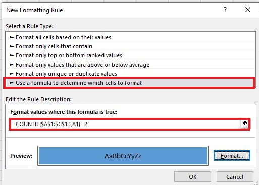
You can use any number or logical operator (<,>, etc) here that you prefer. In this case, the COUNTIF formula returns the number of occurrences where a cell repeats in the data range A1:C13. If the value is equal to two, conditional formatting is applied.
- Choose your preferred Formatting style and Click OK.
How to Find Duplicate Rows in Excel?
Sometimes, you may want to find and highlight duplicate rows of data instead of just cells. I’ll show you a foolproof method to implement this in Excel. Follow these steps.
- Select the Data Range that contains the duplicate rows.
- Clear any existing conditional formatting in your data.
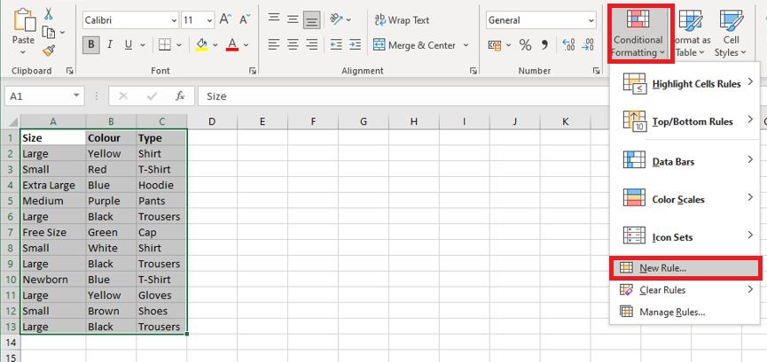
- Under Conditional Formatting, locate and click on the New Rule option.
- In the next window, under the Rule Type select the Use a formula to determine which cells to format option.
- Under “Format Values where this formula is true” I enter =COUNTIFS($A$1:$A$13,$A1,$B$1:$B$13,$B1,$C$1:$C$13,$C1)>1
The COUNTIFS formula checks every column simultaneously for cases where all these duplicate cells repeat in the same row. That is it checks for duplicate rows. Change A1:A13, B1:B13, C1:C13 suitably as per your data range.

- Choose your preferred Formatting Style and Click OK.
How to Remove Duplicate Rows in Excel?
In some cases, just highlighting duplicate rows is not enough. You also need to delete them.
Follow these steps to easily remove duplicate rows.
- Get your data ready
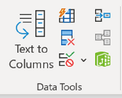
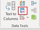
- Locate the Data Tools section under the Data Tab of your Excel Sheet

- Under Data Tools, click on the Remove Duplicates button.
4. Select all the columns for deleting duplicate rows and Click OK. Voila! Excel removes all duplicate rows in just a click.

How to Use COUNTIF / COUNTIFS to Find Duplicates in Excel?
When it comes to handling duplicates, there cannot be a more robust and suitable formula than COUNTIFS. It can be used for granular level actions like finding duplicates excluding the first instance, finding case sensitive duplicates, counting the number of duplicates until each row, etc. I’ll show you how to do all of this with the help of examples.
How to Find Duplicates in Excel Using COUNTIF?
To find duplicates using COUNTIF, follow these steps.
Let’s assume I have the column “A” full of repetitive data and I need to identify these duplicates using the COUNTIF formula.
How to Find Duplicates Including the First Instance?
- Get your Data ready
- In the ‘B2’ cell, i.e right next to column “A”, type in
= IF(COUNTIF($A$2:$A$13,A2)>1,”Yes”,””)
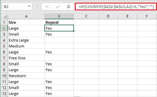
Here, the COUNTIF function compares each cell in the range A2:A13 for duplicates and returns the total number of repetitions for each case. The “IF” function then checks if the number of repetitions is greater than one. If it is greater than one, it is a duplicate, else, not a duplicate.
- Drag this formula to the end of the data range using the fill handle.
- All your duplicate cells are now marked with “YES”
Did you notice that it is marking even the first instances of data as duplicates?
Sometimes this is not required, especially if you are planning to delete or filter the data later. To avoid this from happening, follow the steps below.
How to Find Duplicates Excluding the First Instance?
I am working with the same set of Data in Column “A”
- Get your Data ready.
- In the ‘B2’ cell, i.e right next to column “A”, type in =IF(COUNTIF($A$2:$A2,A2)>1,”Yes”,””)
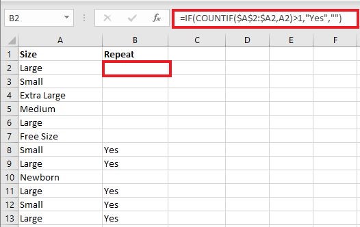
Here, the COUNTIF function searches each Cell in the Data Range of Column “A” for duplicates. It then returns the number of repetitions until that particular row. The IF function then compares if the number of repetitions is greater than one, in order to mark as duplicates. Hence, the first instance of any duplicate will return a value of 1 and the first instance will not be marked as a duplicate.
- Drag the formula to the end of the Data range using the fill handle.
- All your duplicates except the first one are marked with “YES”.
How to Find Case Sensitive Duplicates?
All the above methods consider data with different text-cases as the same and count them as duplicates.
But, sometimes, you may want to find an exactly matching duplicate. To accomplish this, follow these simple steps.
- Get your data ready
- In the ‘B2’ cell, i.e right next to column “A”, type in =IF(SUM((–EXACT($A$2:$A$13,A2)))<=1,””,”Yes”)

Here, the “EXACT” function searches for exact matches to return either 1 or 0. The SUM function returns the total number of exact duplicates. If it is greater than 1, the cell is marked as a duplicate.
- Drag the formula to the end of the Data range using the fill handle.
- All your case sensitive duplicates are marked with “Yes”.
How to Find Duplicate Rows in Excel Using COUNTIFS?
Now, let’s see how to easily find duplicate rows in your sheet using the COUNTIFS functions.
If you want to include the first instance, just follow these simple steps.
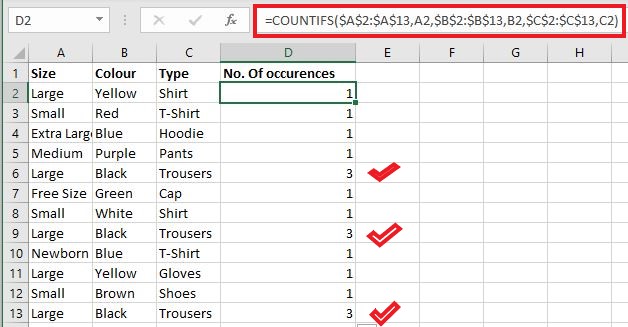
- Get your Data ready. I am using a sheet that contains three columns of data.
- In ‘D2’ cell, i.e right next to the Data enter =IF(COUNTIFS($A$2:$A$13,A2,$B$2:$B$13,B2,$C$2:$C$13,C2)>1, “Yes”, “”)
This is exactly the same as the COUNTIF function, except here it checks all the columns simultaneously for duplicates. Hence, it can find all duplicate rows easily.

- Drag the formula to the end of the data range using the fill handle.
- All your duplicate rows including the first instances are marked with “Yes”
If you want to exclude the first instance, just follow these simple steps
- Get your Data ready, I am using the same Sheet here.
- In ‘D2’ cell, i.e right next to the Data enter =IF(COUNTIFS($A$2:$A2,$A2,$B$2:$B2,$B2,$C$2:$C2,$C2)>1, “Yes”, “”)
Here, the COUNTIFS function compares each row in the data range for duplicates and returns the number of repetitions until that particular row.
The IF function then compares if the number of repetitions is greater than one to mark as duplicates. The first instance of any duplicate will return a value of 1. Hence, the first instance will not be marked as a duplicate

- Drag the formula to the end of the Data range using the fill handle.
- All your duplicate rows excluding the first instances are marked with “Yes”
How to Count Duplicates in Excel Using COUNTIF?
There may be situations where you need to find the number of duplicates in your Data.
Let’s see how to tackle it easily.
How to Count Duplicates for Each Cell?
To count the number of duplicates for each cell just follow these steps.
- Get your Data ready.
- In ‘B2’ Cell, enter =COUNTIF($A$2:$A$13,A2)
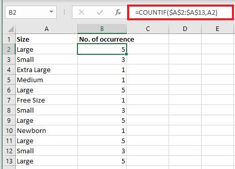
The COUNTIF function simply counts and returns the number of times a single data value gets repeated in the Range A2:A13.
- Drag the formula to the end of the data range using the fill handle.
- All your duplicate data have a corresponding cell that displays their number of occurrences.
How to Count Duplicates for Each Cell Until Each Row?
To count the number of repeats for each cell until each row, follow these steps.
- Get your Data ready
- In ‘B2’ Cell, enter =COUNTIF($A$2:$A$13,A2)
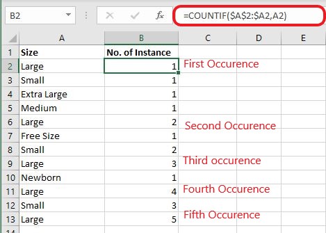
Here, the COUNTIF function searches each Cell in the Data Range of Column “A” for duplicates. It then returns the number of repetitions until that particular row. Hence, we get the number of instances until each row.
- Drag the formula to the end of the data range using the fill handle.
- Each duplicate data has a corresponding cell that displays their number of instances until that row.
How to Count the Number of Duplicate Rows in Excel Using COUNTIFS?
You can use the same methods to find the number of occurrences for duplicate rows. Just use the COUNTIFS functions in the place of the COUNTIF function.
For example, in the following case I enter =COUNTIFS($A$2:$A$13,A2,$B$2:$B$13,B2,$C$2:$C$13,C2) in the “D2” cell to get the desired result
How to Filter Duplicates in Excel?
Finally, you may want to filter all duplicates found in your Sheet. This is a very useful feature that will come in handy if you want to further delete, move or copy these duplicates.
Let’s see how to do this easily. Just follow these steps.
- Select the Data where you already have found the duplicates using the COUNTIFS formula.
- Under the Data Tab, locate and click on the Filter button.
- Now, click on the arrow on the “Repeat” column header and check only “Yes” to show only the duplicates.
- You can also uncheck “Yes” to hide all duplicates.
Do anything as you please with these filtered duplicate rows of data. You can remove, copy to another sheet, or simply hide them.
Suggested Reads:
How To Protect Cells In Excel Workbooks-the Easiest Way
Create An Excel Dashboard In 5 Minutes – The Best Guide
Dynamic Dropdown Lists In Excel – Top Data Validation Guide
FAQs
What is the easiest way to count duplicates in Excel?
The easiest way to count duplicates is to use the COUNTIF function if you already know the value you are looking for.
Just type COUNTIF(X:X, X1) where ‘X’ is the column you want to search and ‘X1’ is the value you are counting for.
How do you find duplicates in Excel and group them together?
The easiest way to group duplicates together in Excel is to highlight them using conditional formatting. Then go to the SORT option under the DATA tab and under the drop-down options click “Cell Colour”. All your highlighted duplicates are grouped together now.
Closing Thoughts
We are at the end of this guide on how to find duplicates in Excel. I have covered almost all important user-friendly ways to find duplicates in Excel. All of these methods will come in handy and will suffice for most users.
If you need more high-quality guides on Excel functions and features check out our free Excel resources section.
If you are interested in gaining in-depth knowledge and practice in Excel try our Excel Courses here.
Adam Lacey

Adam Lacey is an Excel enthusiast and online learning expert. He combines these two passions at Simon Sez IT where he wears a number of different hats.When Adam isn’t fretting about site traffic or Pivot Tables, you’ll find him on the tennis court or in the kitchen cooking up a storm.
Duplicate Values | Triplicates | Duplicate Rows
This example teaches you how to find duplicate values (or triplicates) and how to find duplicate rows in Excel.
Duplicate Values
To find and highlight duplicate values in Excel, execute the following steps.
1. Select the range A1:C10.

2. On the Home tab, in the Styles group, click Conditional Formatting.

3. Click Highlight Cells Rules, Duplicate Values.

4. Select a formatting style and click OK.

Result. Excel highlights the duplicate names.

Note: select Unique from the first drop-down list to highlight the unique names.
Triplicates
By default, Excel highlights duplicates (Juliet, Delta), triplicates (Sierra), etc. (see previous image). Execute the following steps to highlight triplicates only.
1. First, clear the previous conditional formatting rule.
2. Select the range A1:C10.
3. On the Home tab, in the Styles group, click Conditional Formatting.
4. Click New Rule.

5. Select ‘Use a formula to determine which cells to format’.
6. Enter the formula =COUNTIF($A$1:$C$10,A1)=3
7. Select a formatting style and click OK.

Result. Excel highlights the triplicate names.

Explanation: =COUNTIF($A$1:$C$10,A1) counts the number of names in the range A1:C10 that are equal to the name in cell A1. If COUNTIF($A$1:$C$10,A1) = 3, Excel formats cell A1. Always write the formula for the upper-left cell in the selected range (A1:C10). Excel automatically copies the formula to the other cells. Thus, cell A2 contains the formula =COUNTIF($A$1:$C$10,A2)=3, cell A3 =COUNTIF($A$1:$C$10,A3)=3, etc. Notice how we created an absolute reference ($A$1:$C$10) to fix this reference.
Note: you can use any formula you like. For example, use this formula =COUNTIF($A$1:$C$10,A1)>3 to highlight names that occur more than 3 times.
Duplicate Rows
To find and highlight duplicate rows in Excel, use COUNTIFS (with the letter S at the end) instead of COUNTIF.
1. Select the range A1:C10.

2. On the Home tab, in the Styles group, click Conditional Formatting.
3. Click New Rule.
4. Select ‘Use a formula to determine which cells to format’.
5. Enter the formula =COUNTIFS(Animals,$A1,Continents,$B1,Countries,$C1)>1
6. Select a formatting style and click OK.

Note: the named range Animals refers to the range A1:A10, the named range Continents refers to the range B1:B10 and the named range Countries refers to the range C1:C10. =COUNTIFS(Animals,$A1,Continents,$B1,Countries,$C1) counts the number of rows based on multiple criteria (Leopard, Africa, Zambia).
Result. Excel highlights the duplicate rows.

Explanation: if COUNTIFS(Animals,$A1,Continents,$B1,Countries,$C1) > 1, in other words, if there are multiple (Leopard, Africa, Zambia) rows, Excel formats cell A1. Always write the formula for the upper-left cell in the selected range (A1:C10). Excel automatically copies the formula to the other cells. We fixed the reference to each column by placing a $ symbol in front of the column letter ($A1, $B1 and $C1). As a result, cell A1, B1 and C1 contain the same formula, cell A2, B2 and C2 contain the formula =COUNTIFS(Animals,$A2,Continents,$B2,Countries,$C2)>1, etc.
7. Finally, you can use the Remove Duplicates tool in Excel to quickly remove duplicate rows. On the Data tab, in the Data Tools group, click Remove Duplicates.

In the example below, Excel removes all identical rows (blue) except for the first identical row found (yellow).


Note: visit our page about removing duplicates to learn more about this great Excel tool.
Skip to content
В этой статье мы рассмотрим разные подходы к одной из самых распространенных и, по моему мнению, важных задач в Excel — как найти в ячейках и в столбцах таблицы повторяющиеся значения.
Работая с большими наборами данных в Excel или объединяя несколько небольших электронных таблиц в более крупные, вы можете столкнуться с большим числом одинаковых строк.
И сегодня я хотел бы поделиться несколькими быстрыми и эффективными методами выявления дубликатов в одном списке. Эти решения работают во всех версиях Excel 2016, Excel 2013, 2010 и ниже. Вот о чём мы поговорим:
- Поиск повторяющихся значений включая первые вхождения
- Поиск дубликатов без первых вхождений
- Определяем дубликаты с учетом регистра
- Как извлечь дубликаты из диапазона ячеек
- Как обнаружить одинаковые строки в таблице данных
- Использование встроенных фильтров Excel
- Применение условного форматирования
- Поиск совпадений при помощи встроенной команды «Найти»
- Определяем дубликаты при помощи сводной таблицы
- Duplicate Remover — быстрый и эффективный способ найти дубликаты
Самой простой в использовании и вместе с тем эффективной в данном случае будет функция СЧЁТЕСЛИ (COUNTIF). С помощью одной только неё можно определить не только неуникальные позиции, но и их первые появления в столбце. Рассмотрим разницу на примерах.
Поиск повторяющихся значений включая первые вхождения.
Предположим, что у вас в колонке А находится набор каких-то показателей, среди которых, вероятно, есть одинаковые. Это могут быть номера заказов, названия товаров, имена клиентов и прочие данные. Если ваша задача — найти их, то следующая формула для вас:
=СЧЁТЕСЛИ(A:A; A2)>1
Где А2 — первая ячейка из области для поиска.
Просто введите это выражение в любую ячейку и протяните вниз вдоль всей колонки, которую нужно проверить на дубликаты.

Как вы могли заметить на скриншоте выше, формула возвращает ИСТИНА, если имеются совпадения. А для встречающихся только 1 раз значений она показывает ЛОЖЬ.
Подсказка! Если вы ищите повторы в определенной области, а не во всей колонке, обозначьте нужный диапазон и “зафиксируйте” его знаками $. Это значительно ускорит вычисления. Например, если вы ищете в A2:A8, используйте
=СЧЕТЕСЛИ($A$2:$A$8, A2)>1
Если вас путает ИСТИНА и ЛОЖЬ в статусной колонке и вы не хотите держать в уме, что из них означает повторяющееся, а что — уникальное, заверните свою СЧЕТЕСЛИ в функцию ЕСЛИ и укажите любое слово, которое должно соответствовать дубликатам и уникальным:
=ЕСЛИ(СЧЁТЕСЛИ($A$2:$A$17; A2)>1;»Дубликат»;»Уникальное»)
Если же вам нужно, чтобы формула указывала только на дубли, замените «Уникальное» на пустоту («»):

=ЕСЛИ(СЧЁТЕСЛИ($A$2:$A$17; A2)>1;»Дубликат»;»»)

В этом случае Эксель отметит только неуникальные записи, оставляя пустую ячейку напротив уникальных.
Поиск неуникальных значений без учета первых вхождений
Вы наверняка обратили внимание, что в примерах выше дубликатами обозначаются абсолютно все найденные совпадения. Но зачастую задача заключается в поиске только повторов, оставляя первые вхождения нетронутыми. То есть, когда что-то встречается в первый раз, оно однозначно еще не может быть дубликатом.
Если вам нужно указать только совпадения, давайте немного изменим:
=ЕСЛИ(СЧЁТЕСЛИ($A$2:$A2; A2)>1;»Дубликат»;»»)
На скриншоте ниже вы видите эту формулу в деле.

Нетрудно заметить, что она не обозначает первое появление слова, а начинает отсчет со второго.
Чувствительный к регистру поиск дубликатов
Хочу обратить ваше внимание на то, что хоть формулы выше и находят 100%-дубликаты, есть один тонкий момент — они не чувствительны к регистру. Быть может, для вас это не принципиально. Но если в ваших данных абв, Абв и АБВ — это три разных параметра – то этот пример для вас.
Как вы могли уже догадаться, выражения, использованные нами ранее, с такой задачей не справятся. Здесь нужно выполнить более тонкий поиск, с чем нам поможет следующая функция массива:
{=ЕСЛИ(СУММ((—СОВПАД($A$2:$A$17;A2)))<=1;»»;»Дубликат»)}
Не забывайте, что формулы массива вводятся комбиинацией Ctrl + Shift + Enter.
Если вернуться к содержанию, то здесь используется функция СОВПАД для сравнения целевой ячейки со всеми остальными ячейками с выбранной области. Результат возвращается в виде ИСТИНА (совпадение) или ЛОЖЬ (не совпадение), которые затем преобразуются в массив из 1 и 0 при помощи оператора (—).
После этого, функция СУММ складывает эти числа. И если полученный результат больше 1, функция ЕСЛИ сообщает о найденном дубликате.
Если вы взглянете на следующий скриншот, вы убедитесь, что поиск действительно учитывает регистр при обнаружении дубликатов:

Смородина и арбуз, которые встречаются дважды, не отмечены в нашем поиске, так как регистр первых букв у них отличается.
Как извлечь дубликаты из диапазона.
Формулы, которые мы описывали выше, позволяют находить дубликаты в определенном столбце. Но часто речь идет о нескольких столбцах, то есть о диапазоне данных.
Рассмотрим это на примере числовой матрицы. К сожалению, с символьными значениями этот метод не работает.

При помощи формулы массива
{=ИНДЕКС(НАИМЕНЬШИЙ(ЕСЛИ(СЧЁТЕСЛИ($A$2:$E$11;$A$2:$E$11)>1;$A$2:$E$11);СТРОКА($1:$100)); НАИМЕНЬШИЙ(ЕСЛИОШИБКА(ЕСЛИ(ПОИСКПОЗ(НАИМЕНЬШИЙ(ЕСЛИ( СЧЁТЕСЛИ($A$2:$E$11;$A$2:$E$11)>1;$A$2:$E$11);СТРОКА($1:$100)); НАИМЕНЬШИЙ(ЕСЛИ(СЧЁТЕСЛИ($A$2:$E$11;$A$2:$E$11)>1;$A$2:$E$11); СТРОКА($1:$100));0)=СТРОКА($1:$100);СТРОКА($1:$100));»»);СТРОКА()-1))}
вы можете получить упорядоченный по возрастанию список дубликатов. Для этого введите это выражение в нужную ячейку и нажмите Ctrl+Alt+Enter.
Затем протащите маркер заполнения вниз на сколько это необходимо.
Чтобы убрать сообщения об ошибке, когда дублирующиеся значения закончатся, можно использовать функцию ЕСЛИОШИБКА:
=ЕСЛИОШИБКА(ИНДЕКС(НАИМЕНЬШИЙ(ЕСЛИ(СЧЁТЕСЛИ($A$2:$E$11;$A$2:$E$11)>1;$A$2:$E$11); СТРОКА($1:$100));НАИМЕНЬШИЙ(ЕСЛИОШИБКА(ЕСЛИ(ПОИСКПОЗ( НАИМЕНЬШИЙ(ЕСЛИ(СЧЁТЕСЛИ($A$2:$E$11;$A$2:$E$11)>1;$A$2:$E$11); СТРОКА($1:$100));НАИМЕНЬШИЙ(ЕСЛИ(СЧЁТЕСЛИ($A$2:$E$11;$A$2:$E$11)>1;$A$2:$E$11); СТРОКА($1:$100));0)=СТРОКА($1:$100);СТРОКА($1:$100));»»);СТРОКА()-1));»»)
Также обратите внимание, что приведенное выше выражение рассчитано на то, что оно будет записано во второй строке. Соответственно выше него будет одна пустая строка.
Поэтому если вам нужно разместить его, к примеру, в ячейке K4, то выражение СТРОКА()-1 в конце замените на СТРОКА()-3.
Обнаружение повторяющихся строк
Мы рассмотрели, как обнаружить одинаковые данные в отдельных ячейках. А если нужно искать дубликаты-строки?
Есть один метод, которым можно воспользоваться, если вам нужно просто выделить одинаковые строки, но не удалять их.
Итак, имеются данные о товарах и заказчиках.
Создадим справа от наших данных формулу, объединяющую содержание всех расположенных слева от нее ячеек.
Предположим, что данные хранятся в столбцах А:C. Запишем в ячейку D2:
=A2&B2&C2
Добавим следующую формулу в ячейку E2. Она отобразит, сколько раз встречается значение, полученное нами в столбце D:
=СЧЁТЕСЛИ(D:D;D2)
Скопируем вниз для всех строк данных.
В столбце E отображается количество появлений этой строки в столбце D. Неповторяющимся строкам будет соответствовать значение 1. Повторам строкам соответствует значение больше 1, указывающее на то, сколько раз такая строка была найдена.
Если вас не интересует определенный столбец, просто не включайте его в выражение, находящееся в D. Например, если вам хочется обнаружить совпадающие строки, не учитывая при этом значение Заказчик, уберите из объединяющей формулы упоминание о ячейке С2.
Обнаруживаем одинаковые ячейки при помощи встроенных фильтров Excel.
Теперь рассмотрим, как можно обойтись без формул при поиске дубликатов в таблице. Быть может, кому-то этот метод покажется более удобным, нежели написание выражений Excel.
Организовав свои данные в виде таблицы, вы можете применять к ним различные фильтры. Фильтр в таблице вы можете установить по одному либо по нескольким столбцам. Давайте рассмотрим на примере.
В первую очередь советую отформатировать наши данные как «умную» таблицу. Напомню: Меню Главная – Форматировать как таблицу.
После этого в строке заголовка появляются значки фильтра. Если нажать один из них, откроется выпадающее меню фильтра, которое содержит всю информацию по данному столбцу. Выберите любой элемент из этого списка, и Excel отобразит данные в соответствии с этим выбором.
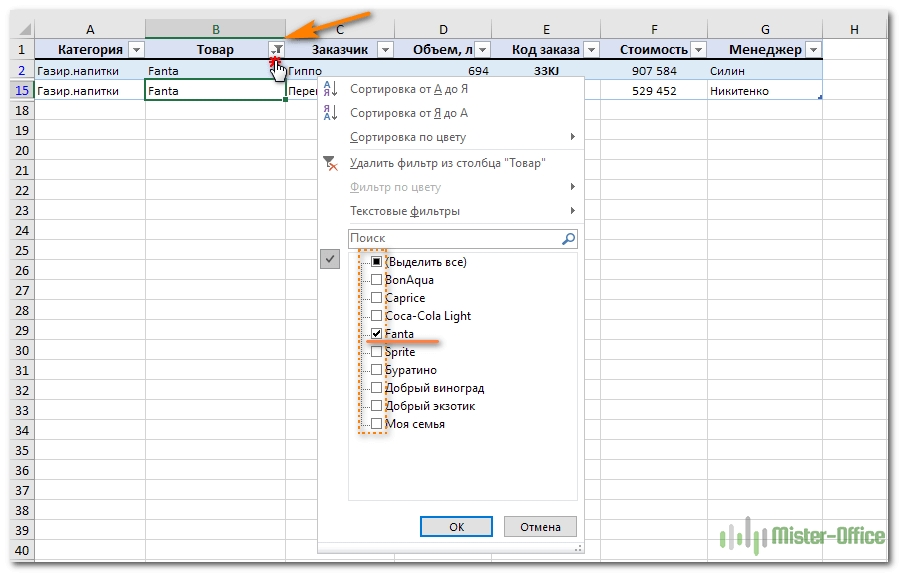
Вы можете убрать галочку с пункта «Выделить все», а затем отметить один или несколько нужных элементов. Excel покажет только те строки, которые содержат выбранные значения. Так можно обнаружить дубликаты, если они есть. И все готово для их быстрого удаления.
Но при этом вы видите дубли только по отфильтрованному. Если данных много, то искать таким способом последовательного перебора будет несколько утомительно. Ведь слишком много раз нужно будет устанавливать и менять фильтр.
Используем условное форматирование.
Выделение цветом по условию – весьма важный инструмент Excel, о котором достаточно подробно мы рассказывали.
Сейчас я покажу, как можно в Экселе найти дубли ячеек, просто их выделив цветом.
Как показано на рисунке ниже, выбираем Правила выделения ячеек – Повторяющиеся. Неуникальные данные будут подсвечены цветом.
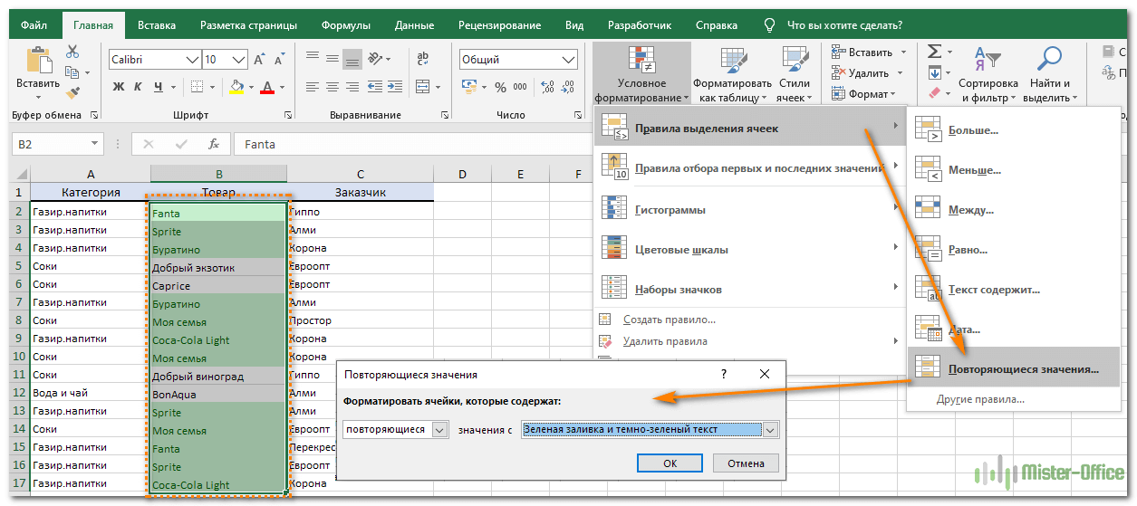
Но здесь мы не можем исключить первые появления – подсвечивается всё.
Но эту проблему можно решить, использовав формулу условного форматирования.
=СЧЁТЕСЛИ($B$2:$B2; B2)>1

Результат работы формулы выденения повторяющихся значений вы видите выше. Они выделены зелёным цветом.
Чтобы освежить память, можете руководствоваться нашим материалом «Как изменить цвет ячейки в зависимости от значения».
Поиск совпадений при помощи команды «Найти».
Еще один простой, но не слишком технологичный способ – использование встроенного поиска.
Зайдите на вкладку Главная и кликните «Найти и выделить». Откроется диалоговое окно, в котором можно ввести что угодно для поиска в таблице. Чтобы избежать опечаток, можете скопировать искомое прямо из списка данных.
Затем нажимаем «Найти все», и видим все найденные дубликаты и места их расположения, как на рисунке чуть ниже.

В случае, когда объём информации очень велик и требуется ускорить работу поиска, предварительно выделите столбец или диапазон, в котором нужно искать, и только после этого начинайте работу. Если этого не сделать, Excel будет искать по всем имеющимся данным, что, конечно, медленнее.
Этот метод еще более трудоемкий, нежели использование фильтра. Поэтому применяют его выборочно, только для отдельных значений.
Как применить сводную таблицу для поиска дубликатов.
Многие считают сводные таблицы слишком сложным инструментом, чтобы постоянно им пользоваться. На самом деле, не все так запутано, как кажется. Для новичков рекомендую к ознакомлению наше руководство по созданию и работе со сводными таблицами.
Для более опытных – сразу переходим к сути вопроса.
Создаем новый макет сводной таблицы. А затем в качестве строк и значений используем одно и то же поле. В нашем случае – «Товар». Поскольку название товара – это текст, то для подсчета таких значений Excel по умолчанию использует функцию СЧЕТ, то есть подсчитывает количество. А нам это и нужно. Если будет больше 1, значит, имеются дубликаты.

Вы наблюдаете на скриншоте выше, что несколько товаров дублируются. И что нам это дает? А далее мы просто можем щелкнуть мышкой на любой из цифр, и на новом листе Excel покажет нам, как получилась эта цифра.
К примеру, откуда взялись 3 дубликата Sprite? Щелкаем на цифре 3, и видим такую картину:

Думаю, этот метод вполне можно использовать. Что приятно – никаких формул не требуется.
Duplicate Remover — быстрый и эффективный способ найти дубликаты в Excel
Теперь, когда вы знаете, как использовать формулы для поиска повторяющихся значений в Excel, позвольте мне продемонстрировать вам еще один быстрый, эффективный и без всяких формул способ: инструмент Duplicate Remover для Excel.
Этот универсальный инструмент может искать повторяющиеся или уникальные значения в одном столбце или же сравнивать два столбца. Он может находить, выбирать и выделять повторяющиеся записи или целые повторяющиеся строки, удалять найденные дубли, копировать или перемещать их на другой лист. Я думаю, что пример практического использования может заменить очень много слов, так что давайте перейдем к нему.
Как найти повторяющиеся строки в Excel за 2 быстрых шага
Сначала посмотрим в работе наиболее простой инструмент — быстрый поиск дубликатов Quick Dedupe. Используем уже знакомую нам таблицу, в которой мы выше искали дубликаты при помощи формул:

Как видите, в таблице несколько столбцов. Чтобы найти повторяющиеся записи в этих трех столбцах, просто выполните следующие действия:
- Выберите любую ячейку в таблице и нажмите кнопку Quick Dedupe на ленте Excel. После установки пакета Ultimate Suite для Excel вы найдете её на вкладке Ablebits Data в группе Dedupe. Это наиболее простой инструмент для поиска дубликатов.
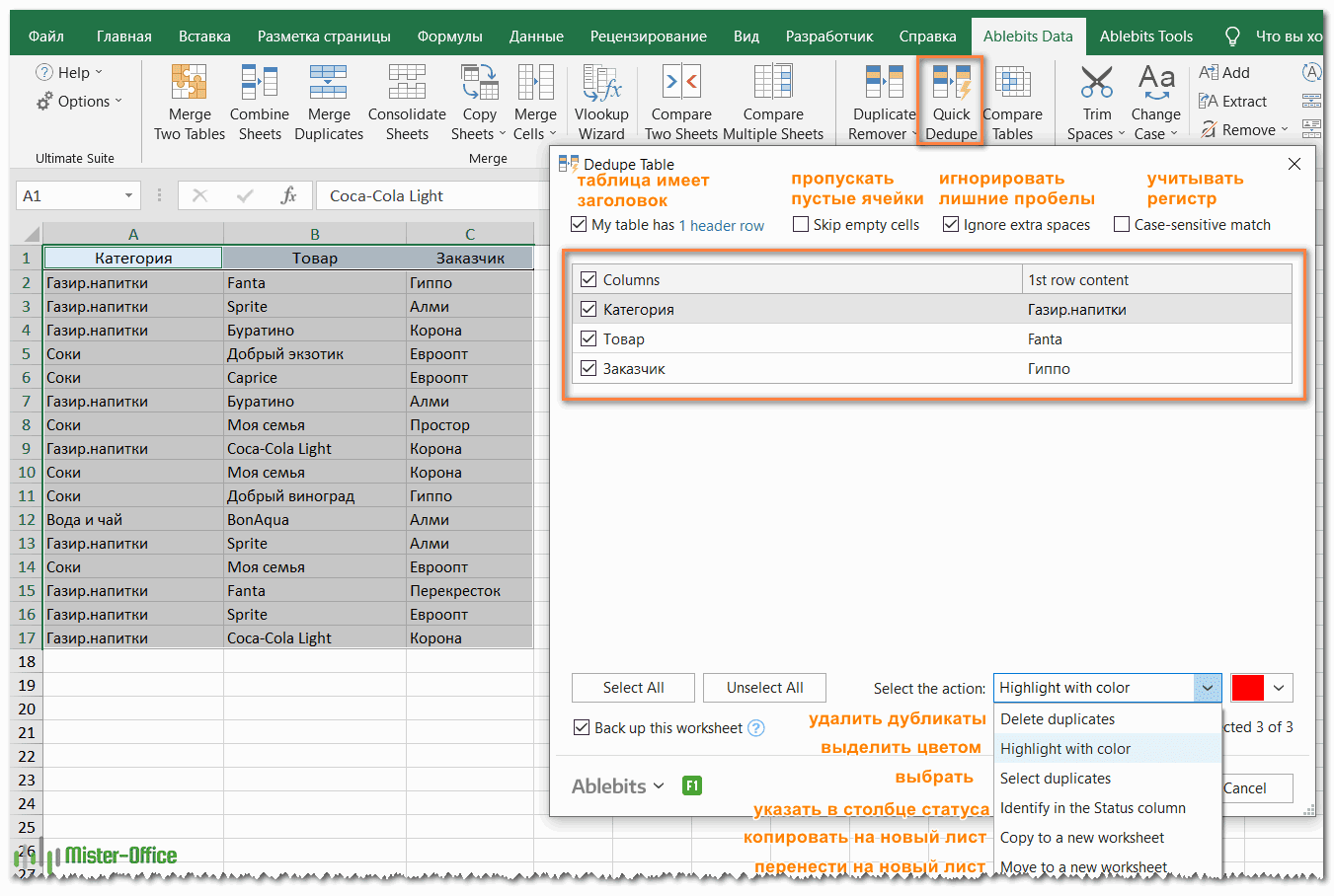
- Интеллектуальная надстройка возьмет всю таблицу и попросит вас указать следующие две вещи:
- Выберите столбцы для проверки дубликатов (в данном примере это все 3 столбца – категория, товар и заказчик).
- Выберите действие, которое нужно выполнить с дубликатами. Поскольку наша цель — выявить повторяющиеся строки, я выбрал «Выделить цветом».
Помимо выделения цветом, вам доступен ряд других опций:
- Удалить дубликаты
- Выбрать дубликаты
- Указать их в столбце статуса
- Копировать дубликаты на новый лист
- Переместить на новый лист
Нажмите кнопку ОК и подождите несколько секунд. Готово! И никаких формул 😊.
Как вы можете видеть на скриншоте ниже, все строки с одинаковыми значениями в первых 3 столбцах были обнаружены (первые вхождения не идентифицируются как дубликаты).

Если вам нужны дополнительные возможности для работы с дубликатами и уникальными значениями, используйте мастер удаления дубликатов Duplicate Remover, который может найти дубликаты с первыми вхождениями или без них, а также уникальные значения. Подробные инструкции приведены ниже.
Мастер удаления дубликатов — больше возможностей для поиска дубликатов в Excel.
В зависимости от данных, с которыми вы работаете, вы можете не захотеть рассматривать первые экземпляры идентичных записей как дубликаты. Одно из возможных решений — использовать разные формулы для каждого сценария, как мы обсуждали в этой статье выше. Если же вы ищете быстрый, точный метод без формул, попробуйте мастер удаления дубликатов — Duplicate Remover. Несмотря на свое название, он не только умеет удалять дубликаты, но и производит с ними другие полезные действия, о чём мы далее поговорим подробнее. Также умеет находить уникальные значения.
- Выберите любую ячейку в таблице и нажмите кнопку Duplicate Remover на вкладке Ablebits Data.
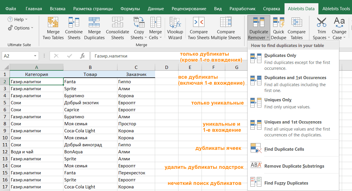
- Вам предложены 4 варианта проверки дубликатов в вашем листе Excel:
- Дубликаты без первых вхождений повторяющихся записей.
- Дубликаты с 1-м вхождением.
- Уникальные записи.
- Уникальные значения и 1-е повторяющиеся вхождения.
В этом примере выберем второй вариант, т.е. Дубликаты + 1-е вхождения:

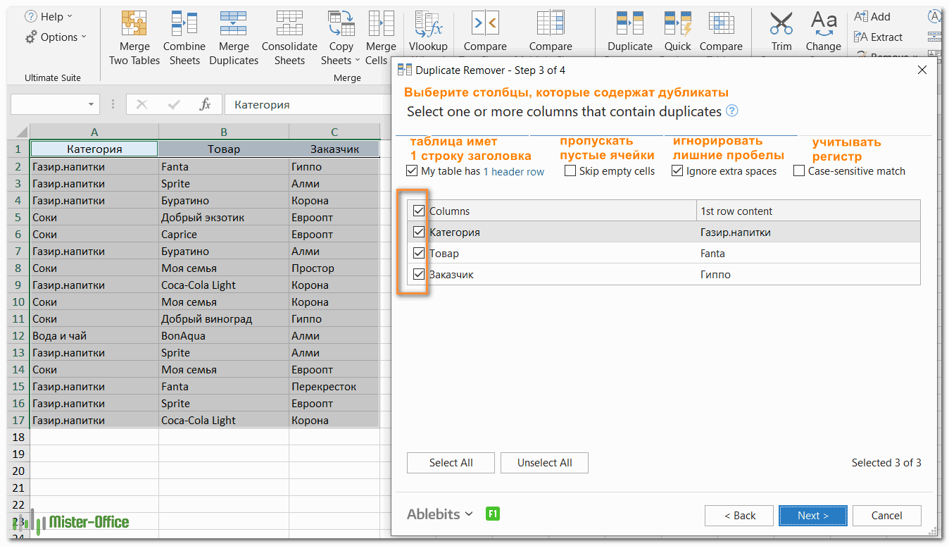
- Теперь выберите столбцы, в которых вы хотите проверить дубликаты. Как и в предыдущем примере, мы возьмём первые 3 столбца:
- Наконец, выберите действие, которое вы хотите выполнить с дубликатами. Как и в случае с инструментом быстрого поиска дубликатов, мастер Duplicate Remover может идентифицировать, выбирать, выделять, удалять, копировать или перемещать повторяющиеся данные.

Поскольку цель этого примера – продемонстрировать различные способы определения дубликатов в Excel, давайте отметим параметр «Выделить цветом» (Highlight with color) и нажмите Готово.
Мастеру Duplicate Remover требуется всего лишь несколько секунд, чтобы проверить вашу таблицу и показать результат:

Как видите, результат аналогичен предыдущему. Но здесь мы выделили дубликаты, включая и первое появление повторяющихся записей.
Никаких формул, никакого стресса, никаких ошибок — всегда быстрые и безупречные результаты 
Итак, мы с вам научились различными способами обнаруживать повторяющиеся записи в таблице Excel. В следующих статьях разберем, что мы с этим можем полезного сделать.
Если вы хотите попробовать эти инструменты для поиска дубликатов в таблицах Excel, вы можете загрузить полнофункциональную ознакомительную версию программы. Будем очень признательны за ваши отзывы в комментариях!
In MS Excel, the duplicate values can be found and removed from a data set. Depending on your data and requirement, the most commonly used methods are the conditional formatting feature or the COUNTIF formula to find and highlight the duplicates for a specific number of occurences. The columns of the data set can be then filtered to view the duplicate values.
In this article, we will look at 5 different methods to check, identify, and delete duplicates in Excel.
Table of contents
- How to Find Duplicates in Excel?
- 5 Methods to Check & Identify Duplicates in Excel
- #1 – Conditional Formatting
- #2 – Conditional Formatting (Specific Occurrence)
- #3 – Change Rules (Formulas)
- #4 – Remove Duplicates
- #5 – COUNTIF Formula
- Frequently Asked Questions
- Recommended Articles
- 5 Methods to Check & Identify Duplicates in Excel
5 Methods to Check & Identify Duplicates in Excel
You can download this Find for Duplicates Excel Template here – Find for Duplicates Excel Template
#1 – Conditional Formatting
The conditional formattingConditional formatting is a technique in Excel that allows us to format cells in a worksheet based on certain conditions. It can be found in the styles section of the Home tab.read more feature is available in Excel 2007 and subsequent versions.
The following table consists of the expenses incurred on availing certain office facilities. The corresponding dates of purchasing such facility are also listed.
We want to identify the duplicates in excel with the help of conditional formatting.
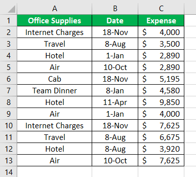
The steps to find the duplicates in excel with the help of conditional formatting are listed as follows:
- Select the data range (A1:C13) where duplicates are to be found.
- In the Home tab, select “conditional formatting” from the “styles” section. From the drop-down menu, select “highlight cell rules” and click on “duplicate values.”

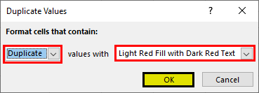
- The pop-up window titled “duplicate values” appears. In the first box on the left side, select “duplicate.” In the “values with” drop-down, select the required color to highlight the duplicate cells. Click “Ok.”

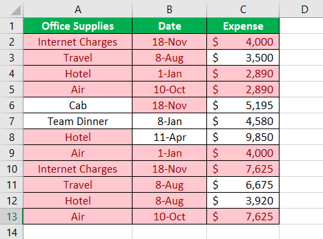
- The duplicate cells are highlighted in the data table, as shown in the following image.

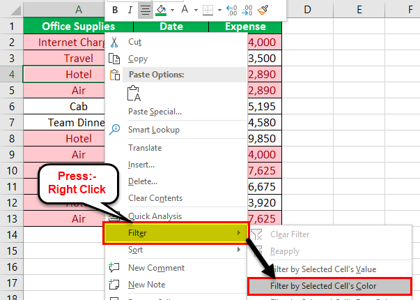
- The columns can be filtered to identify the duplicate values. For this, right-click the required column and select “filter by selected cell’s color.” The data is filtered for duplicates.

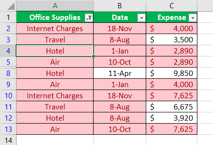
- The result after applying the filter to the first column (office supplies) is shown in the following image.

#2 – Conditional Formatting (Specific Occurrence)
Let us consider an example to identify the specific number of duplications. In the following table, we want to check and show the duplicate values with three occurrences.
The steps to find the duplicate values for specific number of occurrences are listed as follows:
Step 1: Select the range A2:C8 in the given data table.
Step 2: In the Home tab, select “conditional formatting” from the “styles” section. Click “new rule.”
Note: The “new rule” option helps highlight a specific count of duplicates using the COUNTIF formula.
Step 3: The pop-up window titled “new formatting rule” appears. Enter the following details, as shown in the succeeding image.
- Under “select a rule type,” select “use a formula to determine which cells to format.”
- Under “edit the rule description,” enter the COUNTIFThe COUNTIF function in Excel counts the number of cells within a range based on pre-defined criteria. It is used to count cells that include dates, numbers, or text. For example, COUNTIF(A1:A10,”Trump”) will count the number of cells within the range A1:A10 that contain the text “Trump”
read more formula.
The COUNTIF formula “=COUNTIF(cell range of the data table, cell criteria)” finds and highlights the cells for the desired number of occurrences.
In this case, the COUNTIF formula highlights duplicate cells having triplicate count. This count can be changed to a greater number. The conditions can also be changed depending on the user’s requirement.
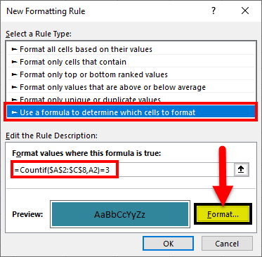
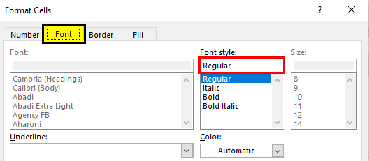
Step 4: Once the COUNTIF formula is entered, click “format.” The pop-up window titled “format cells” opens. Select the font style “regular.”
Step 5: In the “fill” tab, select blue color. The “fill” tab helps highlight the duplicate cellsHighlight Cells Rule, which is available under Conditional Formatting under the Home menu tab, can be used to highlight duplicate values in the selected dataset, whether it is a column or row of a table.read more.
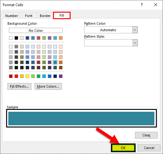
Step 6: Once the selections in “format cells” window are complete, click “Ok.” Click “Ok” again in the “new formatting rule” window.
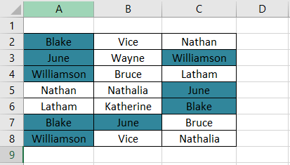
Step 7: The result is displayed in the following image. The duplicate cells with three occurrences are highlighted.
#3 – Change Rules (Formulas)
Working on the data of example #2, let us understand the procedure of changing the formula. For applying new formulas, the existing rules (formulas) of the data tableA data table in excel is a type of what-if analysis tool that allows you to compare variables and see how they impact the result and overall data. It can be found under the data tab in the what-if analysis section.read more have to be cleared.
The steps to clear the existing rules (shown in the succeeding image) are listed as follows:
Step 1: In the Home tab, select “conditional formatting” from the “styles” section.
Step 2: In “clear rules” option, select either of the following:
- Clear rules from selected cells–This resets the rules for the selected range of the table. So, prior to clearing the rules, the data needs to be selected.
- Clear rules from entire sheet–This clears the rules for the entire sheet.
The blue highlighted cells disappear and the original table is displayed.
#4 – Remove Duplicates
Let us check and delete duplicate values from a selected range. Prior to deletion, keeping a copy of the table is advisable because the duplicates will be permanently deleted.
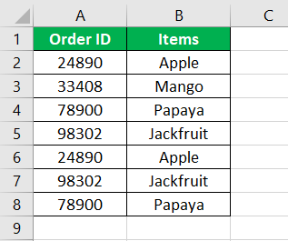
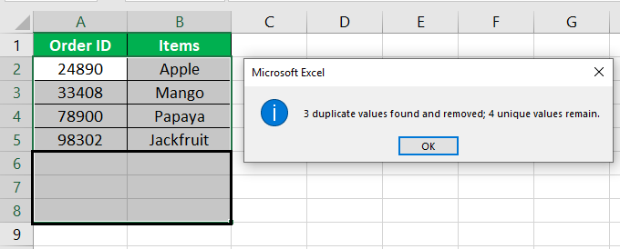
The following table displays a series of items with their corresponding IDs.
The steps to find and delete duplicate values are listed as follows:
Step 1: Select the range of the table whose duplicates are required to be deleted.
Step 2: In the Data tab, select “remove duplicates” from the “data tools” section.
Note: The “remove duplicates” option helps eliminate duplicates and retain unique cell values.
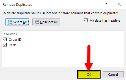
Step 3: The pop-up window titled “remove duplicates” appears, as shown in the succeeding image. By default, the following options are already selected:
- The checkboxes for both the headers (“order ID” and “items”)
- The “select all” box
Since the table consists of column headers, select the checkbox “my data has headers.” Click “Ok” to execute.
Note: To change the number of columns selected, click “unselect all.” Following this, the desired columns from which the duplicates are to be deleted can be selected.
Step 4: The result is shown in the succeeding image. A prompt is displayed which states the following details:
- The number of duplicate values removed from the table
- The number of unique values that remain in the table after deletion
Click “Ok.” Hence, the duplicate values along with their corresponding rows are deleted.
#5 – COUNTIF Formula
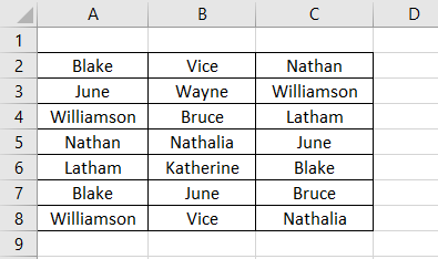
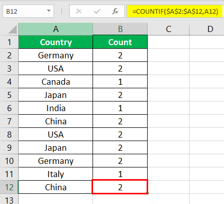
The following table displays the names of a few countries. We want to identify the duplicate values using the COUNTIF function.
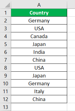
The COUNTIF function requires the range (column containing duplicate entries) and the cell criteria. It returns the number of corresponding duplicates for every cell.
The steps to find the duplicate values in excel with the help of the COUNTIF function are listed as follows:
Step 1: Enter the formula shown in the succeeding image. Press the “Enter” key.
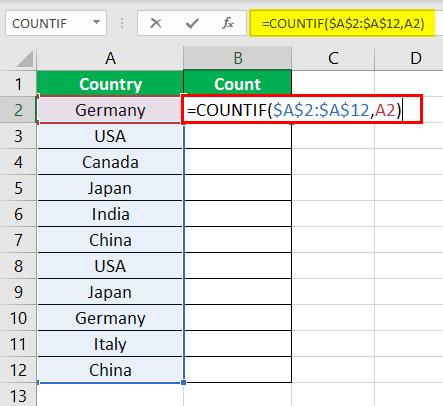
Note: The range must be fixed with the dollar ($) sign. Otherwise, the cell reference will change on dragging the formula.
Step 2: Drag the formula till the end of the table with the help of the fill handle. Alternatively, place the cursor on cell B2 and double-click the fill handle. The fill handle appears at the lower right corner of cell B2.
Step 3: The output of the formula is shown in the following image. It returns the count of duplicates for the entire data set.
Note: The filter can be applied to the column header to view the occurrences greater than one.
Frequently Asked Questions
1. What does it mean to find duplicates in Excel?
While consolidating different worksheets, several duplicates may be found in a data set. MS Excel helps to find and highlight such duplicates. It is also possible to filter a column for duplicate values.
An easy way to search for duplicates is by using the COUNTIF formula. This formula can count the total number of duplicates in a column. It can also count the number of individual instances of a particular duplicate entry. It accepts two arguments–the range and the criteria.
2. How to find duplicates in a column of Excel?
To check a column for duplicates, the formula is given as follows:
“=COUNTIF(A:A,A2)>1”
The formula checks for duplicates in column A. The topmost cell is A2. For every duplicate value, the formula returns “true.” For every unique value, the formula returns “false.”
Note: For an output other than “true” and “false,” the COUNTIF formula can be enclosed in the IF function.
3. What is the formula to find duplicates in Excel?
The generic formula to find the exact, case-sensitive duplicate values is stated as follows:
“IF(SUM((-EXACT(range,uppermost_cell)))<=1,””,”Duplicate”)”
The EXACT function compares the cell range with the target cell. The SUM function adds the number of instances. If the occurrence is greater than 1, the IF function returns “duplicate.”
Note 1: Since it is an array formula, it should be entered using “Ctrl+Shift+Enter.”
Note 2: If the same word appears twice in lowercase and once in uppercase, the formula will not count the uppercase word as duplicate.
Recommended Articles
This has been a guide to Find Duplicates in Excel. Here we discuss how to identify, check and show duplicates in excel with examples. You may also look at these useful functions in Excel –
- How to Use IF Formula in Excel (with Examples)?
- Conditional Formatting for Blank Cells | Steps
- Create a Dashboard in Excel
- Apply Conditional Formatting in Pivot Table