Excel find all cells with value - Word и Excel - помощь в работе с программами

Summary

This step-by-step article describes how to find data in a table (or range of cells) by using various built-in functions in Microsoft Excel. You can use different formulas to get the same result.

Create the Sample Worksheet

This article uses a sample worksheet to illustrate Excel built-in functions. Consider the example of referencing a name from column A and returning the age of that person from column C. To create this worksheet, enter the following data into a blank Excel worksheet.

You will type the value that you want to find into cell E2. You can type the formula in any blank cell in the same worksheet.

	A	B	C	D	E
1	Name	Dept	Age		Find Value
2	Henry	501	28		Mary
3	Stan	201	19
4	Mary	101	22
5	Larry	301	29

Term Definitions

This article uses the following terms to describe the Excel built-in functions:

Term	Definition	Example
Table Array	The whole lookup table	A2:C5
Lookup_Value	The value to be found in the first column of Table_Array.	E2
Lookup_Array -or- Lookup_Vector	The range of cells that contains possible lookup values.	A2:A5
Col_Index_Num	The column number in Table_Array the matching value should be returned for.	3 (third column in Table_Array)
Result_Array -or- Result_Vector	A range that contains only one row or column. It must be the same size as Lookup_Array or Lookup_Vector.	C2:C5
Range_Lookup	A logical value (TRUE or FALSE). If TRUE or omitted, an approximate match is returned. If FALSE, it will look for an exact match.	FALSE
Top_cell	This is the reference from which you want to base the offset. Top_Cell must refer to a cell or range of adjacent cells. Otherwise, OFFSET returns the #VALUE! error value.
Offset_Col	This is the number of columns, to the left or right, that you want the upper-left cell of the result to refer to. For example, «5» as the Offset_Col argument specifies that the upper-left cell in the reference is five columns to the right of reference. Offset_Col can be positive (which means to the right of the starting reference) or negative (which means to the left of the starting reference).

Functions

LOOKUP()

The LOOKUP function finds a value in a single row or column and matches it with a value in the same position in a different row or column.

The following is an example of LOOKUP formula syntax:

=LOOKUP(Lookup_Value,Lookup_Vector,Result_Vector)

The following formula finds Mary’s age in the sample worksheet:

=LOOKUP(E2,A2:A5,C2:C5)

The formula uses the value «Mary» in cell E2 and finds «Mary» in the lookup vector (column A). The formula then matches the value in the same row in the result vector (column C). Because «Mary» is in row 4, LOOKUP returns the value from row 4 in column C (22).

NOTE: The LOOKUP function requires that the table be sorted.

For more information about the LOOKUP function, click the following article number to view the article in the Microsoft Knowledge Base:

How to use the LOOKUP function in Excel

VLOOKUP()

The VLOOKUP or Vertical Lookup function is used when data is listed in columns. This function searches for a value in the left-most column and matches it with data in a specified column in the same row. You can use VLOOKUP to find data in a sorted or unsorted table. The following example uses a table with unsorted data.

The following is an example of VLOOKUP formula syntax:

=VLOOKUP(Lookup_Value,Table_Array,Col_Index_Num,Range_Lookup)

The following formula finds Mary’s age in the sample worksheet:

=VLOOKUP(E2,A2:C5,3,FALSE)

The formula uses the value «Mary» in cell E2 and finds «Mary» in the left-most column (column A). The formula then matches the value in the same row in Column_Index. This example uses «3» as the Column_Index (column C). Because «Mary» is in row 4, VLOOKUP returns the value from row 4 in column C (22).

For more information about the VLOOKUP function, click the following article number to view the article in the Microsoft Knowledge Base:

How to Use VLOOKUP or HLOOKUP to find an exact match

INDEX() and MATCH()

You can use the INDEX and MATCH functions together to get the same results as using LOOKUP or VLOOKUP.

The following is an example of the syntax that combines INDEX and MATCH to produce the same results as LOOKUP and VLOOKUP in the previous examples:

=INDEX(Table_Array,MATCH(Lookup_Value,Lookup_Array,0),Col_Index_Num)

The following formula finds Mary’s age in the sample worksheet:

=INDEX(A2:C5,MATCH(E2,A2:A5,0),3)

The formula uses the value «Mary» in cell E2 and finds «Mary» in column A. It then matches the value in the same row in column C. Because «Mary» is in row 4, the formula returns the value from row 4 in column C (22).

NOTE: If none of the cells in Lookup_Array match Lookup_Value («Mary»), this formula will return #N/A.
For more information about the INDEX function, click the following article number to view the article in the Microsoft Knowledge Base:

How to use the INDEX function to find data in a table

OFFSET() and MATCH()

You can use the OFFSET and MATCH functions together to produce the same results as the functions in the previous example.

The following is an example of syntax that combines OFFSET and MATCH to produce the same results as LOOKUP and VLOOKUP:

=OFFSET(top_cell,MATCH(Lookup_Value,Lookup_Array,0),Offset_Col)

This formula finds Mary’s age in the sample worksheet:

=OFFSET(A1,MATCH(E2,A2:A5,0),2)

The formula uses the value «Mary» in cell E2 and finds «Mary» in column A. The formula then matches the value in the same row but two columns to the right (column C). Because «Mary» is in column A, the formula returns the value in row 4 in column C (22).

For more information about the OFFSET function, click the following article number to view the article in the Microsoft Knowledge Base:

How to use the OFFSET function

Need more help?

Want more options?

Explore subscription benefits, browse training courses, learn how to secure your device, and more.

Communities help you ask and answer questions, give feedback, and hear from experts with rich knowledge.

Источник

See all How-To Articles

In this tutorial, you will learn how to select all cells with values in Excel.

Select All Cells With Values

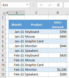
In Excel, it’s easy to select all cells in a sheet or range, but it’s also possible to select all cells containing values at once with just a little more work. Say you have the data set below, with some values missing for Sales Amount (Column D). The following example will show how to select all cells in the range at once, excluding those without values.

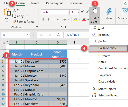
Select the entire range (e.g., B3:D12) and in the Ribbon, go to Home > Find & Select > Go To Special.

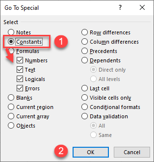
In the Go To Special window, select Constants and click OK.
When you select Constants, Numbers, Text, Logicals, and Errors are all checked by default. This means that all four types of data will be selected. If there are some types you don’t want to include, uncheck them.

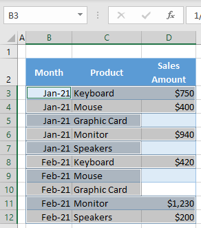
As a result, cells that are not empty are selected, while empty cells (D5, D7, D9, and D10) are not.

Summary

To search an entire worksheet for a value and return a count, you can use a formula based on the COUNTIF function.

In the example shown, the formula in C5 is:

=COUNTIF(Sheet2!1:1048576,C4)

Generic formula

Explanation

The second sheet in the workbook, Sheet2, contains 1000 first names in the range B4:F203.

The COUNTIF function takes a range and a criteria. In this case, we give COUNTIF a range equal to all rows in Sheet2.

Sheet2!1:1048576

Note: an easy way to enter this range is to use the Select All button.

For criteria, we use a reference to C4, which contains «John». COUNTIF then returns 15, since there are 15 cells in Sheet2 equal to «John».

Contains vs. Equals

If you want to count all cells that contain the value in C4, instead of all cells equal to C4, add the wildcards to the criteria like this:

=COUNTIF(Sheet2!1:1048576,"*"&C4&"*")

Now COUNTIF will count cells with the substring «John» anywhere in the cell.

Performance

In general, it’s not a good practice to specify a range that includes all worksheet cells. Doing so can cause major performance problems, since the range includes millions and millions of cells. When possible, restrict the range to a sensible area.

Author

Dave Bruns

Hi — I’m Dave Bruns, and I run Exceljet with my wife, Lisa. Our goal is to help you work faster in Excel. We create short videos, and clear examples of formulas, functions, pivot tables, conditional formatting, and charts.

There are hundreds and hundreds of Excel sites out there. I’ve been to many and most are an exercise in frustration. Found yours today and wanted to let you know that it might be the simplest and easiest site that will get me where I want to go.

Get Training

Quick, clean, and to the point training

Learn Excel with high quality video training. Our videos are quick, clean, and to the point, so you can learn Excel in less time, and easily review key topics when needed. Each video comes with its own practice worksheet.

View Paid Training & Bundles

Help us improve Exceljet

Источник

Поиск какого-либо значения в ячейках Excel довольно часто встречающаяся задача при программировании какого-либо макроса. Решить ее можно разными способами. Однако, в разных ситуациях использование того или иного способа может быть не оправданным. В данной статье я рассмотрю 2 наиболее распространенных способа.

Поиск перебором значений

Довольно простой в реализации способ. Например, найти в колонке «A» ячейку, содержащую «123» можно примерно так:

Sheets("Данные").Select
For y = 1 To Cells.SpecialCells(xlLastCell).Row
    If Cells(y, 1) = "123" Then
        Exit For
    End If
Next y
MsgBox "Нашел в строке: " + CStr(y)

Минусами этого так сказать «классического» способа являются: медленная работа и громоздкость. А плюсом является его гибкость, т.к. таким способом можно реализовать сколь угодно сложные варианты поиска с различными вычислениями и т.п.

Поиск функцией Find

Гораздо быстрее обычного перебора и при этом довольно гибкий. В простейшем случае, чтобы найти в колонке A ячейку, содержащую «123» достаточно такого кода:

Sheets("Данные").Select
Set fcell = Columns("A:A").Find("123")
If Not fcell Is Nothing Then
    MsgBox "Нашел в строке: " + CStr(fcell.Row)
End If

Вкратце опишу что делают строчки данного кода:
1-я строка: Выбираем в книге лист «Данные»;
2-я строка: Осуществляем поиск значения «123» в колонке «A», результат поиска будет в fcell;
3-я строка: Если удалось найти значение, то fcell будет содержать Range-объект, в противном случае — будет пустой, т.е. Nothing.

Полностью синтаксис оператора поиска выглядит так:

Find(What, After, LookIn, LookAt, SearchOrder, SearchDirection, MatchCase, MatchByte, SearchFormat)

What — Строка с текстом, который ищем или любой другой тип данных Excel

After — Ячейка, после которой начать поиск. Обратите внимание, что это должна быть именно единичная ячейка, а не диапазон. Поиск начинается после этой ячейки, а не с нее. Поиск в этой ячейке произойдет только когда весь диапазон будет просмотрен и поиск начнется с начала диапазона и до этой ячейки включительно.

LookIn — Тип искомых данных. Может принимать одно из значений: xlFormulas (формулы), xlValues (значения), или xlNotes (примечания).

LookAt — Одно из значений: xlWhole (полное совпадение) или xlPart (частичное совпадение).

SearchOrder — Одно из значений: xlByRows (просматривать по строкам) или xlByColumns (просматривать по столбцам)

SearchDirection — Одно из значений: xlNext (поиск вперед) или xlPrevious (поиск назад)

MatchCase — Одно из значений: True (поиск чувствительный к регистру) или False (поиск без учета регистра)

MatchByte — Применяется при использовании мультибайтных кодировок: True (найденный мультибайтный символ должен соответствовать только мультибайтному символу) или False (найденный мультибайтный символ может соответствовать однобайтному символу)

SearchFormat — Используется вместе с FindFormat. Сначала задается значение FindFormat (например, для поиска ячеек с курсивным шрифтом так: Application.FindFormat.Font.Italic = True), а потом при использовании метода Find указываем параметр SearchFormat = True. Если при поиске не нужно учитывать формат ячеек, то нужно указать SearchFormat = False.

Чтобы продолжить поиск, можно использовать FindNext (искать «далее») или FindPrevious (искать «назад»).

Примеры поиска функцией Find

Пример 1: Найти в диапазоне «A1:A50» все ячейки с текстом «asd» и поменять их все на «qwe»

With Worksheets(1).Range("A1:A50")
  Set c = .Find("asd", LookIn:=xlValues)
  Do While Not c Is Nothing
    c.Value = "qwe"
    Set c = .FindNext(c)
  Loop
End With

Обратите внимание: Когда поиск достигнет конца диапазона, функция продолжит искать с начала диапазона. Таким образом, если значение найденной ячейки не менять, то приведенный выше пример зациклится в бесконечном цикле. Поэтому, чтобы этого избежать (зацикливания), можно сделать следующим образом:

Пример 2: Правильный поиск значения с использованием FindNext, не приводящий к зацикливанию.

With Worksheets(1).Range("A1:A50")
  Set c = .Find("asd", lookin:=xlValues)
  If Not c Is Nothing Then
    firstResult = c.Address
    Do
      c.Font.Bold = True
      Set c = .FindNext(c)
      If c Is Nothing Then Exit Do
    Loop While c.Address <> firstResult
  End If
End With

В ниже следующем примере используется другой вариант продолжения поиска — с помощью той же функции Find с параметром After. Когда найдена очередная ячейка, следующий поиск будет осуществляться уже после нее. Однако, как и с FindNext, когда будет достигнут конец диапазона, Find продолжит поиск с его начала, поэтому, чтобы не произошло зацикливания, необходимо проверять совпадение с первым результатом поиска.

Пример 3: Продолжение поиска с использованием Find с параметром After.

With Worksheets(1).Range("A1:A50")
  Set c = .Find("asd", lookin:=xlValues)
  If Not c Is Nothing Then
    firstResult = c.Address
    Do
      c.Font.Bold = True
      Set c = .Find("asd", After:=c, lookin:=xlValues)
      If c Is Nothing Then Exit Do
    Loop While c.Address <> firstResult
  End If
End With

Следующий пример демонстрирует применение SearchFormat для поиска по формату ячейки. Для указания формата необходимо задать свойство FindFormat.

Пример 4: Найти все ячейки с шрифтом «курсив» и поменять их формат на обычный (не «курсив»)

lLastRow = Cells.SpecialCells(xlLastCell).Row
lLastCol = Cells.SpecialCells(xlLastCell).Column
Application.FindFormat.Font.Italic = True
With Worksheets(1).Range(Cells(1, 1), Cells(lLastRow, lLastCol))
  Set c = .Find("", SearchFormat:=True)
  Do While Not c Is Nothing
    c.Font.Italic = False
    Set c = .Find("", After:=c, SearchFormat:=True)
  Loop
End With

Примечание: В данном примере намеренно не используется FindNext для поиска следующей ячейки, т.к. он не учитывает формат (статья об этом: https://support.microsoft.com/ru-ru/kb/282151)

Коротко опишу алгоритм поиска Примера 4. Первые две строки определяют последнюю строку (lLastRow) на листе и последний столбец (lLastCol). 3-я строка задает формат поиска, в данном случае, будем искать ячейки с шрифтом Italic. 4-я строка определяет область ячеек с которой будет работать программа (с ячейки A1 и до последней строки и последнего столбца). 5-я строка осуществляет поиск с использованием SearchFormat. 6-я строка — цикл пока результат поиска не будет пустым. 7-я строка — меняем шрифт на обычный (не курсив), 8-я строка продолжаем поиск после найденной ячейки.

Хочу обратить внимание на то, что в этом примере я не стал использовать «защиту от зацикливания», как в Примерах 2 и 3, т.к. шрифт меняется и после «прохождения» по всем ячейкам, больше не останется ни одной ячейки с курсивом.

Свойство FindFormat можно задавать разными способами, например, так:

With Application.FindFormat.Font 
  .Name = "Arial" 
  .FontStyle = "Regular" 
  .Size = 10 
End With

Поиск последней заполненной ячейки с помощью Find

Следующий пример — применение функции Find для поиска последней ячейки с заполненными данными. Использованные в Примере 4 SpecialCells находит последнюю ячейку даже если она не содержит ничего, но отформатирована или в ней раньше были данные, но были удалены.

Пример 5: Найти последнюю колонку и столбец, заполненные данными

Set c = Worksheets(1).UsedRange.Find("*", SearchDirection:=xlPrevious)
If Not c Is Nothing Then
  lLastRow = c.Row: lLastCol = c.Column 
Else
  lLastRow = 1: lLastCol = 1
End If
MsgBox "lLastRow=" & lLastRow & " lLastCol=" & lLastCol

В этом примере используется UsedRange, который так же как и SpecialCells возвращает все используемые ячейки, в т.ч. и те, что были использованы ранее, а сейчас пустые. Функция Find ищет ячейку с любым значением с конца диапазона.

Поиск по шаблону (маске)

При поиске можно так же использовать шаблоны, чтобы найти текст по маске, следующий пример это демонстрирует.

Пример 6: Выделить красным шрифтом ячейки, в которых текст начинается со слова из 4-х букв, первая и последняя буквы «т», при этом после этого слова может следовать любой текст.

With Worksheets(1).Cells
  Set c = .Find("т??т*", LookIn:=xlValues, LookAt:=xlWhole)
  If Not c Is Nothing Then
    firstResult = c.Address
    Do
      c.Font.Color = RGB(255, 0, 0)
      Set c = .FindNext(c)
      If c Is Nothing Then Exit Do
    Loop While c.Address <> firstResult
  End If
End With

Для поиска функцией Find по маске (шаблону) можно применять символы:
* — для обозначения любого количества любых символов;
? — для обозначения одного любого символа;
~ — для обозначения символов *, ? и ~. (т.е. чтобы искать в тексте вопросительный знак, нужно написать ~?, чтобы искать именно звездочку (*), нужно написать ~* и наконец, чтобы найти в тексте тильду, необходимо написать ~~)

Поиск в скрытых строках и столбцах

Для поиска в скрытых ячейках нужно учитывать лишь один нюанс: поиск нужно осуществлять в формулах, а не в значениях, т.е. нужно использовать LookIn:=xlFormulas

Поиск даты с помощью Find

Если необходимо найти текущую дату или какую-то другую дату на листе Excel или в диапазоне с помощью Find, необходимо учитывать несколько нюансов:

Тип данных Date в VBA представляется в виде #[месяц]/[день]/[год]#, соответственно, если необходимо найти фиксированную дату, например, 01 марта 2018 года, необходимо искать #3/1/2018#, а не «01.03.2018»
В зависимости от формата ячеек, дата может выглядеть по-разному, поэтому, чтобы искать дату независимо от формата, поиск нужно делать не в значениях, а в формулах, т.е. использовать LookIn:=xlFormulas

Приведу несколько примеров поиска даты.

Пример 7: Найти текущую дату на листе независимо от формата отображения даты.

d = Date
Set c = Cells.Find(d, LookIn:=xlFormulas, LookAt:=xlWhole)
If Not c Is Nothing Then
  MsgBox "Нашел"
Else
  MsgBox "Не нашел"
End If

Пример 8: Найти 1 марта 2018 г.

d = #3/1/2018#
Set c = Cells.Find(d, LookIn:=xlFormulas, LookAt:=xlWhole)
If Not c Is Nothing Then
  MsgBox "Нашел"
Else
  MsgBox "Не нашел"
End If

Искать часть даты — сложнее. Например, чтобы найти все ячейки, где месяц «март», недостаточно искать «03» или «3». Не работает с датами так же и поиск по шаблону. Единственный вариант, который я нашел — это выбрать формат в котором месяц прописью для ячеек с датами и искать слово «март» в xlValues.

Тем не менее, можно найти, например, 1 марта независимо от года.

Пример 9: Найти 1 марта любого года.

d = #3/1/1900#
Set c = Cells.Find(Format(d, "m/d/"), LookIn:=xlFormulas, LookAt:=xlPart)
If Not c Is Nothing Then
  MsgBox "Нашел"
Else
  MsgBox "Не нашел"
End If

Источник

Summary

Create the Sample Worksheet

Term Definitions

Functions

LOOKUP()

VLOOKUP()

INDEX() and MATCH()

OFFSET() and MATCH()

Need more help?

Want more options?

Select All Cells With Values

See also

Summary

Generic formula

Explanation

Contains vs. Equals

Performance

Dave Bruns

Get Training

Quick, clean, and to the point training

Help us improve Exceljet

Поиск перебором значений

Поиск функцией Find

Примеры поиска функцией Find

Поиск последней заполненной ячейки с помощью Find

Поиск по шаблону (маске)

Поиск в скрытых строках и столбцах

Поиск даты с помощью Find