Excel financial function in - Word и Excel - помощь в работе с программами

To get detailed information about a function, click its name in the first column.

Note: Version markers indicate the version of Excel a function was introduced. These functions aren’t available in earlier versions. For example, a version marker of 2013 indicates that this function is available in Excel 2013 and all later versions.

Function	Description
ACCRINT function	Returns the accrued interest for a security that pays periodic interest
ACCRINTM function	Returns the accrued interest for a security that pays interest at maturity
AMORDEGRC function	Returns the depreciation for each accounting period by using a depreciation coefficient
AMORLINC function	Returns the depreciation for each accounting period
COUPDAYBS function	Returns the number of days from the beginning of the coupon period to the settlement date
COUPDAYS function	Returns the number of days in the coupon period that contains the settlement date
COUPDAYSNC function	Returns the number of days from the settlement date to the next coupon date
COUPNCD function	Returns the next coupon date after the settlement date
COUPNUM function	Returns the number of coupons payable between the settlement date and maturity date
COUPPCD function	Returns the previous coupon date before the settlement date
CUMIPMT function	Returns the cumulative interest paid between two periods
CUMPRINC function	Returns the cumulative principal paid on a loan between two periods
DB function	Returns the depreciation of an asset for a specified period by using the fixed-declining balance method
DDB function	Returns the depreciation of an asset for a specified period by using the double-declining balance method or some other method that you specify
DISC function	Returns the discount rate for a security
DOLLARDE function	Converts a dollar price, expressed as a fraction, into a dollar price, expressed as a decimal number
DOLLARFR function	Converts a dollar price, expressed as a decimal number, into a dollar price, expressed as a fraction
DURATION function	Returns the annual duration of a security with periodic interest payments
EFFECT function	Returns the effective annual interest rate
FV function	Returns the future value of an investment
FVSCHEDULE function	Returns the future value of an initial principal after applying a series of compound interest rates
INTRATE function	Returns the interest rate for a fully invested security
IPMT function	Returns the interest payment for an investment for a given period
IRR function	Returns the internal rate of return for a series of cash flows
ISPMT function	Calculates the interest paid during a specific period of an investment
MDURATION function	Returns the Macauley modified duration for a security with an assumed par value of $100
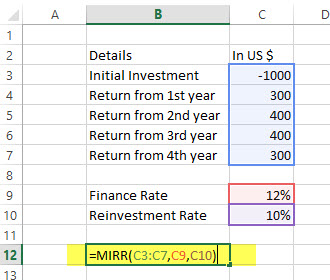
MIRR function	Returns the internal rate of return where positive and negative cash flows are financed at different rates
NOMINAL function	Returns the annual nominal interest rate
NPER function	Returns the number of periods for an investment
NPV function	Returns the net present value of an investment based on a series of periodic cash flows and a discount rate
ODDFPRICE function	Returns the price per $100 face value of a security with an odd first period
ODDFYIELD function	Returns the yield of a security with an odd first period
ODDLPRICE function	Returns the price per $100 face value of a security with an odd last period
ODDLYIELD function	Returns the yield of a security with an odd last period
PDURATION function	Returns the number of periods required by an investment to reach a specified value
PMT function	Returns the periodic payment for an annuity
PPMT function	Returns the payment on the principal for an investment for a given period
PRICE function	Returns the price per $100 face value of a security that pays periodic interest
PRICEDISC function	Returns the price per $100 face value of a discounted security
PRICEMAT function	Returns the price per $100 face value of a security that pays interest at maturity
PV function	Returns the present value of an investment
RATE function	Returns the interest rate per period of an annuity
RECEIVED function	Returns the amount received at maturity for a fully invested security
RRI function	Returns an equivalent interest rate for the growth of an investment
SLN function	Returns the straight-line depreciation of an asset for one period
SYD function	Returns the sum-of-years’ digits depreciation of an asset for a specified period
TBILLEQ function	Returns the bond-equivalent yield for a Treasury bill
TBILLPRICE function	Returns the price per $100 face value for a Treasury bill
TBILLYIELD function	Returns the yield for a Treasury bill
VDB function	Returns the depreciation of an asset for a specified or partial period by using a declining balance method
XIRR function	Returns the internal rate of return for a schedule of cash flows that is not necessarily periodic
XNPV function	Returns the net present value for a schedule of cash flows that is not necessarily periodic
YIELD function	Returns the yield on a security that pays periodic interest
YIELDDISC function	Returns the annual yield for a discounted security; for example, a Treasury bill
YIELDMAT function	Returns the annual yield of a security that pays interest at maturity

Important: The calculated results of formulas and some Excel worksheet functions may differ slightly between a Windows PC using x86 or x86-64 architecture and a Windows RT PC using ARM architecture. Learn more about the differences.

Источник

Microsoft Excel is the most important tool of Investment Bankers Investment banking is a specialized banking stream that facilitates the business entities, government and other organizations in generating capital through debts and equity, reorganization, mergers and acquisition, etc.read moreand Financial Analysts. They spent more than 70% of the time preparing Excel Models, formulating Assumptions, Valuations, Calculations, Graphs, etc. It is safe to assume that Investment bankers are masters in excel shortcuts and formulas. Though there are more than 50+ Financial Functions in Excel, here is the list of Top 15 financial functions in excel that are most frequently used in practical situations.

Without much ado, let’s have a look at all the financial functions one by one –

Top 15 Financial Functions in Excel
#1 – Future Value (FV): Financial Function in Excel
- FV Example
#2 – FVSCHEDULE: Financial Function in Excel
- FVSCHEDULE Example:
#3 – Present Value (PV): Financial Function in Excel
- PV Example:
#4 – Net Present Value (NPV): Financial Function in Excel
- NPV Example
#5 – XNPV: Financial Function in Excel
- XNPV Example
#6 – PMT: Financial Function in Excel
- PMT Example
#7 – PPMT: Financial Function in Excel
- PPMT Example
#8 – Internal Rate of Return (IRR): Financial Function in Excel
- IRR Example
#9 – Modified Internal Rate of Return (MIRR): Financial Function in Excel
- MIRR Example
#10 – XIRR: Financial Function in Excel
- XIRR Example
#11 – NPER: Financial Function in Excel
- NPER Example
#12 – RATE: Financial Function in Excel
- RATE Example
#13 – EFFECT: Financial Function in Excel
- EFFECT Example
#14 – NOMINAL: Financial Function in Excel
- NOMINAL Example
#15 – SLN: Financial Function in Excel
- SLN Example
- Top 15 Financial Functions in Excel Video
- Recommended Articles

#1 – Future Value (FV): Financial Function in Excel

If you want to find out the future value of a particular investment which has a constant interest rate and periodic payment, use the following formula –

FV (Rate, Nper, [Pmt], PV, [Type])

Rate = It is the interest rate/period
Nper = Number of periods
[Pmt] = Payment/period
PV = Present Value
[Type] = When the payment is made (if nothing is mentioned, it’s assumed that the payment has been made at the end of the period)

FV Example

A has invested the US $100 in 2016. The payment has been made yearly. The interest rate is 10% p.a. What would be the FV in 2019?

Solution: In excel, we will put the equation as follows –

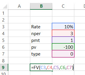
= FV (10%, 3, 1, – 100)

= US $129.79

#2 – FVSCHEDULE: Financial Function in Excel

This financial function is important when you need to calculate the future valueThe Future Value (FV) formula is a financial terminology used to calculate cash flow value at a futuristic date compared to the original receipt. The objective of the FV equation is to determine the future value of a prospective investment and whether the returns yield sufficient returns to factor in the time value of money.read more with the variable interest rateVariable interest rate refers to a mortgage or loan interest rate that fluctuates with the market conditions. The interest levied on variable loans depends on the reference or benchmark rate—an index.
read more. Have a look at the function below –

FVSCHEDULE = (Principal, Schedule)

Principal = Principal is the present value of a particular investment
Schedule = A series of interest rate put together (in case of excel, we will use different boxes and select the range)

FVSCHEDULE Example:

M has invested the US $100 at the end of 2016. It is expected that the interest rate will change every year. In 2017, 2018 & 2019, the interest rates would be 4%, 6% & 5% respectively. What would be the FV in 2019?

Solution: In excel, we will do the following –

= FVSCHEDULE (C1, C2: C4)

= US $115.752

#3 – Present Value (PV): Financial Function in Excel

If you know how to calculate FV, it’s easier for you to find out PV. Here’s how –

PV = (Rate, Nper, [Pmt], FV, [Type])

Rate = It is the interest rate/period
Nper = Number of periods
[Pmt] = Payment/period
FV = Future Value
[Type] = When the payment is made (if nothing is mentioned, it’s assumed that the payment has been made at the end of the period)

PV Example:

The future value of an investment in the US $100 in 2019. The payment has been made yearly. The interest rate is 10% p.a. What would be the PV as of now?

Solution: In excel, we will put the equation as follows –

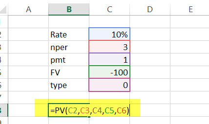
= PV (10%, 3, 1, – 100)

= US $72.64

#4 – Net Present Value (NPV): Financial Function in Excel

Net Present Value is the sum total of positive and negative cash flowsNegative cash flow refers to the situation when cash spending of the company is more than cash generation in a particular period under consideration. This implies that the total cash inflow from the various activities under consideration is less than the total outflow during the same period.read more over the years. Here’s how we will represent it in excel –

NPV = (Rate, Value 1, [Value 2], [Value 3]…)

Rate = Discount rate for a period
Value 1, [Value 2], [Value 3]… = Positive or negative cash flows
Here, negative values would be considered as payments, and positive values would be treated as inflows.

NPV Example

Here is a series of data from which we need to find NPV –

Details	In US $
Rate of Discount	5%
Initial Investment	-1000
Return from 1^st year	300
Return from 2^nd year	400
Return from 3^rd year	400
Return from 4^th year	300

Find out the NPV.

Solution: In Excel, we will do the following –

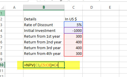
=NPV (5%, B4:B7) + B3

= US $240.87

Also, have a look at this article – NPV vs IRRThe Net Present Value (NPV) method calculates the dollar value of future cash flows which the project will produce during the particular period of time whereas the internal rate of return (IRR) calculates the profitability of the project.read more

#5 – XNPV: Financial Function in Excel

This financial function is similar to the NPV with a twist. Here the payment and income are not periodic. Rather specific dates are mentioned for each payment and income. Here’s how we will calculate it –

XNPV = (Rate, Values, Dates)

Rate = Discount rate for a period
Values = Positive or negative cash flows (an array of values)
Dates = Specific dates (an array of dates)

XNPV Example

Here is a series of data from which we need to find NPV –

Details	In US $	Dates
Rate of Discount	5%
Initial Investment	-1000	1^st December 2011
Return from 1^st year	300	1^st January 2012
Return from 2^nd year	400	1^st February 2013
Return from 3^rd year	400	1^st March 2014
Return from 4^th year	300	1^st April 2015

Solution: In excel, we will do as follows –

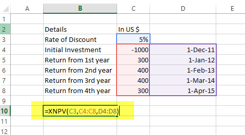
=XNPV (5%, B2:B6, C2:C6)

= US$289.90

#6 – PMT: Financial Function in Excel

In excel, PMT denotes the periodical payment required to pay off for a particular period of time with a constant interest rate. Let’s have a look at how to calculate it in excel –

PMT = (Rate, Nper, PV, [FV], [Type])

Rate = It is the interest rate/period
Nper = Number of periods
PV = Present Value
[FV] = An optional argument which is about the future value of a loan (if nothing is mentioned, FV is considered as “0”)
[Type] = When the payment is made (if nothing is mentioned, it’s assumed that the payment has been made at the end of the period)

PMT Example

The US $1000 needs to be paid in full in 3 years. The interest rate is 10% p.a. and the payment needs to be done yearly. Find out the PMT.

Solution: In excel, we will calculate it in the following manner –

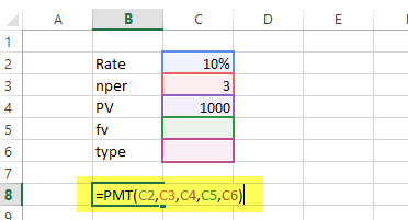
= PMT (10%, 3, 1000)

= – 402.11

#7 – PPMT: Financial Function in Excel

It is another version of PMT. The only difference is this – PPMT calculates payment on principal with a constant interest rate and constant periodic payments. Here’s how to calculate PPMT –

PPMT = (Rate, Per, Nper, PV, [FV], [Type])

Rate = It is the interest rate/period
Per = The period for which the principal is to be calculated
Nper = Number of periods
PV = Present Value
[FV] = An optional argument which is about the future value of a loan (if nothing is mentioned, FV is considered as “0”)
[Type] = When the payment is made (if nothing is mentioned, it’s assumed that the payment has been made at the end of the period)

PPMT Example

The US $1000 needs to be paid in full in 3 years. The interest rate is 10% p.a. and the payment needs to be done yearly. Find out the PPMT in the first year and second year.

Solution: In excel, we will calculate it in the following manner –

1^st year,

=PPMT (10%, 1, 3, 1000)

= US $-302.11

2^nd year,

=PPMT (10%, 2, 3, 1000)

= US $-332.33

#8 – Internal Rate of Return (IRR): Financial Function in Excel

To understand whether any new project or investment is profitable or not, the firm uses IRR. If IRR is more than the hurdle rateThe hurdle rate in capital budgeting is the minimum acceptable rate of return (MARR) on any project or investment required by the manager or investor. It is also known as the company’s required rate of return or target rate.read more (acceptable rate/ average cost of capital), then it’s profitable for the firm and vice-versa. Let’s have a look, how we find out IRR in excel –

IRR = (Values, [Guess])

Values = Positive or negative cash flows (an array of values)
[Guess] = An assumption of what you think IRR should be

IRR Example

Here is a series of data from which we need to find IRR –

Details	In US $
Initial Investment	-1000
Return from 1^st year	300
Return from 2^nd year	400
Return from 3^rd year	400
Return from 4^th year	300

Find out IRR.

Solution: Here’s how we will calculate IRR in excelThe internal rate of return, or IRR, calculates the profit generated by a financial investment. IRR is a built-in function in Excel that calculates the IRR using a range of values as an input and an estimate value as the second input.read more –

= IRR (A2:A6, 0.1)

= 15%

#9 – Modified Internal Rate of Return (MIRR): Financial Function in Excel

The Modified Internal Rate of Return is one step ahead of the Internal Rate of Return. MIRR signifies that the investment is profitable and is used in business. MIRRMIRR or Modified Internal Rate of Return refers to the financial metric used to assess precisely the value and profitability of a potential investment or project. It enables companies and investors to pick the best project or investment based on expected returns. It is nothing but the modified form of the Internal Rate of Return (IRR).read more is calculated by assuming NPV as zero. Here’s how to calculate MIRR in excelMIRR or (modified internal rate of return) in excel is an in-build financial function to calculate the MIRR for the cash flows supplied with a period. It takes the initial investment, interest rate and the interest earned from the earned amount and returns the MIRR.read more –

MIRR = (Values, Finance rate, Reinvestment rate)

Values = Positive or negative cash flows (an array of values)
Finance rate = Interest rate paid for the money used in cash flowsCash Flow is the amount of cash or cash equivalent generated & consumed by a Company over a given period. It proves to be a prerequisite for analyzing the business’s strength, profitability, & scope for betterment. read more
Reinvestment rate = Interest rate paid for reinvestment of cash flows

MIRR Example

Here is a series of data from which we need to find MIRR –

Details	In US $
Initial Investment	-1000
Return from 1^st year	300
Return from 2^nd year	400
Return from 3^rd year	400
Return from 4^th year	300

Finance rate = 12%; Reinvestment rate = 10%. Find out IRR.

Solution: Let’s look at the calculation of MIRR –

= MIRR (B2:B6, 12%, 10%)

= 13%

#10 – XIRR: Financial Function in Excel

Here we need to find out IRR, which has specific dates of cash flow. That’s the only difference between IRR and XIRRIRR function determines the internal rate of return on the cash flows after considering the discount rate and evaluates the return on investment over some time. In contrast, the XIRR function is the extended internal rate of return that considers cash flows and discount rates to measure the return accurately.read more. Have a look at how to calculate XIRR in excelThe XIRR function, also known as the Extended Internal Rate of Return function in Excel, is used to calculate returns based on multiple investments made for a series of non-periodic cash flows.read more financial function –

XIRR = (Values, Dates, [Guess])

Values = Positive or negative cash flows (an array of values)
Dates = Specific dates (an array of dates)
[Guess] = An assumption of what you think IRR should be

XIRR Example

Here is a series of data from which we need to find XIRR –

Details	In US $	Dates


Initial Investment	-1000	1^st December 2011
Return from 1^st year	300	1^st January 2012
Return from 2^nd year	400	1^st February 2013
Return from 3^rd year	400	1^st March 2014
Return from 4^th year	300	1^st April 2015

Solution: Let’s have a look at the solution –

= XIRR (B2:B6, C2:C6, 0.1)

= 24%

#11 – NPER: Financial Function in Excel

It is simply the number of periods one requires to pay off the loan. Let’s see how we can calculate NPER in excelNPER, commonly known as the number of payment periods for a loan, is a financial term and an inbuilt financial function in Excel that can be used to calculate NPER for any loan. This formula takes rate, payment made, present value and future value as input from a user.read more –

NPER = (Rate, PMT, PV, [FV], [Type])

Rate = It is the interest rate/period
PMT = Amount paid per period
PV = Present Value
[FV] = An optional argument which is about the future value of a loan (if nothing is mentioned, FV is considered as “0”)
[Type] = When the payment is made (if nothing is mentioned, it’s assumed that the payment has been made at the end of the period)

NPER Example

US $200 is paid per year for a loan of US $1000. The interest rate is 10% p.a. and the payment needs to be done yearly. Find out the NPER.

Solution: We need to calculate NPER in the following manner –

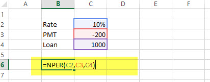
= NPER (10%, -200, 1000)

= 7.27 years

#12 – RATE: Financial Function in Excel

Through the RATE function in excelRate function in excel is used to calculate the rate levied on a period of a loan. The required inputs for this function are number of payment periods, pmt, present value and future value.read more, we can calculate the interest rate needed to pay off the loan in full for a given period of time. Let’s have a look at how to calculate RATE financial function in excel –

RATE = (NPER, PMT, PV, [FV], [Type], [Guess])

Nper = Number of periods
PMT = Amount paid per period
PV = Present Value
[FV] = An optional argument which is about the future value of a loan (if nothing is mentioned, FV is considered as “0”)
[Type] = When the payment is made (if nothing is mentioned, it’s assumed that the payment has been made at the end of the period)
[Guess] = An assumption of what you think RATE should be

RATE Example

US $200 is paid per year for a loan of US $1000 for 6 years, and the payment needs to be done yearly. Find out the RATE.

Solution:

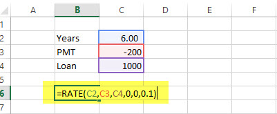
= RATE (6, -200, 1000, 0.1)

= 5%

#13 – EFFECT: Financial Function in Excel

Through the EFFECT function, we can understand the effective annual interest rate. When we have the nominal interest rate and the number of compounding per year, it becomes easy to find out the effective rate. Let’s have a look at how to calculate EFFECT financial function in excel –

EFFECT = (Nominal_Rate, NPERY)

Nominal_Rate = Nominal Interest Rate
NPERY = Number of compounding per year

EFFECT Example

Payment needs to be paid with a nominal interest rateNominal Interest rate refers to the interest rate without the adjustment of inflation. It is a short term interest rate which is used by the central banks to issue loans.read more of 12% when the number of compounding per year is 12.

Solution:

= EFFECT (12%, 12)

= 12.68%

#14 – NOMINAL: Financial Function in Excel

When we have an effective annual rate and the number of compounding periods per year, we can calculate the NOMINAL rate for the year. Let’s have a look at how to do it in excel –

NOMINAL = (Effect_Rate, NPERY)

Effect_Rate = Effective annual interest rate
NPERY = Number of compounding per year

NOMINAL Example

Payment needs to be paid with an effective interest rateEffective Interest Rate, also called Annual Equivalent Rate, is the actual rate of interest that a person pays or earns on a financial instrument by considering the compounding interest over a given period.read more or annual equivalent rate of 12% when the number of compounding per year is 12.

Solution:

= NOMINAL (12%, 12)

= 11.39%

#15 – SLN: Financial Function in Excel

Through the SLN function, we can calculate depreciation via a straight-line method. In excel, we will look at SLN financial function as follows –

SLN = (Cost, Salvage, Life)

Cost = Cost of an asset when bought (initial amount)
Salvage = Value of asset after depreciation
Life = Number of periods over which the asset is being depreciated

SLN Example

The initial cost of machinery is US $5000. It has been depreciated in the Straight Line MethodStraight Line Depreciation Method is one of the most popular methods of depreciation where the asset uniformly depreciates over its useful life and the cost of the asset is evenly spread over its useful and functional life. read more. The machinery was used for 10 years, and now the salvage value of the machinerySalvage value or scrap value is the estimated value of an asset after its useful life is over. For example, if a company’s machinery has a 5-year life and is only valued $5000 at the end of that time, the salvage value is $5000.read more is the US $300. Find depreciation charged per year.

Solution:

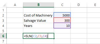
= SLN (5000, 300, 10)

= US $470 per year

You may also look at Depreciation Complete GuideDepreciation is a systematic allocation method used to account for the costs of any physical or tangible asset throughout its useful life. Its value indicates how much of an asset’s worth has been utilized. Depreciation enables companies to generate revenue from their assets while only charging a fraction of the cost of the asset in use each year.
read more

1. FV Function

FV function returns the future value of an investment using constant payments and a constant interest rate. In simple words, it will return a future value of an investment where you have constant payments and a constant interest rate throughout the investment period.

Syntax

FV(rate,nper,pmt,[pv],[type])

Arguments

rate: A constant interest rate that you want to use in the calculation.
nper: Number of payments.
pmt: A constant payment amount to pay periodically throughout the investment time.
[pv]: The present value of future payments. It must be entered as a negative value. 0 if omitted.
[type]: A number to specify when payment is due. 0 = at the end of the period, 1 = at the beginning of the period.

Notes

If pmt is the cash which you have paid (i.e deposits to saving, etc), the value must be negative; and if it is the cash received (income, dividends), the value must be positive.
Make sure you have a specified rate and number of payments in a consistent manner. If the rate is for an annual basis then you have to specify payment periods on an annual basis as well and if you want to specify payments on a monthly basis you have to convert interest rate on a monthly basis by dividing by 12. Same for a quarterly and half-yearly basis.

Example

In the below example, we have used 10% interest rate, 5 payments on a yearly basis, $1000 payment amount, no PV amount and payment type at the beginning of the period. And the function has return 6716 in the result.

Let me explain to you the phenomena working behind the FV.

At the beginning of each period, it will calculate the interest on payment and carry forward that amount (Actual Amount + Interest) to the next period. And in the next period again the same calculation will be done and so on. The best part of FV is that it can do this step by step calculation for you in a single cell.

In the below example, we have used monthly payments.

For this, we have converted the annual interest rate into a month by dividing by 12 and 60 months instead of 5 years and then, specified 10000 for payment. Note: You can also calculate compound interest with FV.

2. PMT

PMT function returns a periodic payment of loan which you need to pay. In simple words, it calculates the loan payment based on fixed monthly payments and a constant rate of interest (loan payment based on fixed monthly payments and a constant rate of interest).

Syntax

PMT(rate, nper, pv, [fv], [type])

Arguments

rate: The rate of interest for the loan. This rate of interest should be constant.
nper: The total number of payments.
pv: The present value or the total amount of loan.
[fv]: The future value or the cash balance which you want after the last payment. The default value is 0.
[type]: Use 0 or 1 to specify the due time of payment. You can use 0 when payment is due at the end of each payment or 1 if payment is due at the start of each period. If you omit to specify the type, it will assume 0.

Notes

The amount of payment return by PMT only includes payment and interest but not include taxes and other fees which are related to the loan.
You have to be sure while specifying the value for rate and nper arguments. If you want to pay monthly installments on a five-year loan at an annual interest rate of 8 percent, use 8%/12 for rate and 5*12 for nper. For annual payments on the same loan, use 8 percent for rate and 5 for nper.

Example

Let’s say you want to take a 20 years mortgage loan for $250000 by assuming 2.5% as an interest rate. Now here we can use PMT to calculate your monthly installments.

In the above calculation, we have converted the annual interest rate into monthly by dividing with 12 and years into months by multiplying with 12.

But we have not mentioned any future value, and the payment type is a default. So as a result, we have got a negative value, because the amount of $987.80 is what we have to pay every month for 30 years.

3. PV

PV Function returns the present value of a financial investment or a loan. In simple words, with the PV function you can calculate the present value of an investment or a loan where you can check is that.

Syntax

PV(rate, nper, pmt, [fv], [type])

Arguments

rate: The rate of interest for the payment of the loan.
nper: Total number of payment periods
pmt: A constant amount of payment you have to make after every period.
[FV]: The future value or a cash balance of a loan or investment you want to attain after the last payment is made. If omitted, it will be assumed as 0.
[type]: Time of the payment. Beginning of the period (use “0”) or the end of the period (Use “1”).

Notes

The units you use as arguments should be consistent. For example, If you are using periods in months (36 Months = 3 Years) then you have to convert the annual interest rate into a monthly interest rate (6%/12 = 0.5%).
PV function is an annuity function. In annuity functions, the cash payments by you are represented by negative numbers and the payments you receive are represented by positive numbers.

Example

Let’s say you want to invest $4000 in an investment plan and in return, you’ll get $1000 at the end of each year for the next 5 years. That means you’ll get a total of $5000 in the next 5 years. Now the thing is, you have to evaluate that this investment is profitable or not. You are investing $4000 today and the return will come to you in the next 5 years.

In the above calculation, it has returned -4329. The present value of your investment is $4329 and you are investing $4000 for it. Hence, your investment is profitable.

Выполнение расчетов с помощью финансовых функций

В группу данных операторов входит более 50 формул. Мы отдельно остановимся на десяти самых востребованных из них. Но прежде давайте рассмотрим, как открыть перечень финансового инструментария для перехода к выполнению решения конкретной задачи.

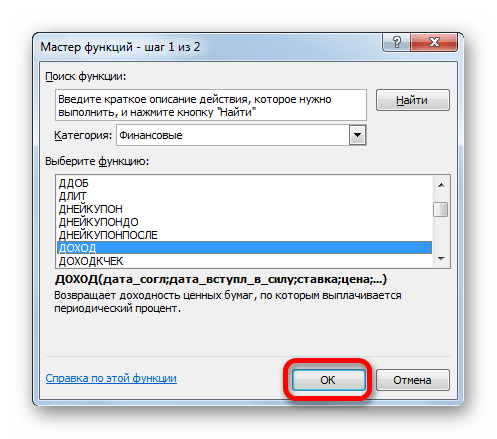
Переход к данному набору инструментов легче всего совершить через Мастер функций.

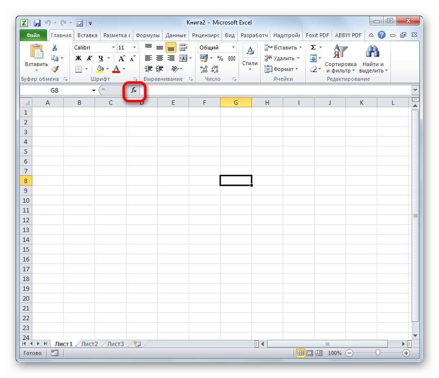
Выделяем ячейку, куда будут выводиться результаты расчета, и кликаем по кнопке «Вставить функцию», находящуюся около строки формул.

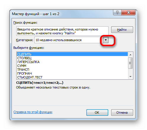
Запускается Мастер функций. Выполняем клик по полю «Категории».

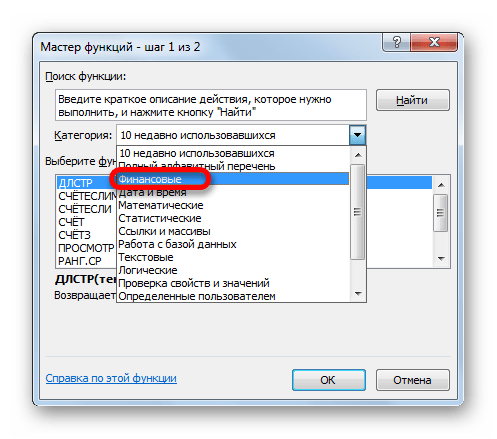
Открывается список доступных групп операторов. Выбираем из него наименование «Финансовые».

Запускается перечень нужных нам инструментов. Выбираем конкретную функцию для выполнения поставленной задачи и жмем на кнопку «OK». После чего открывается окно аргументов выбранного оператора.

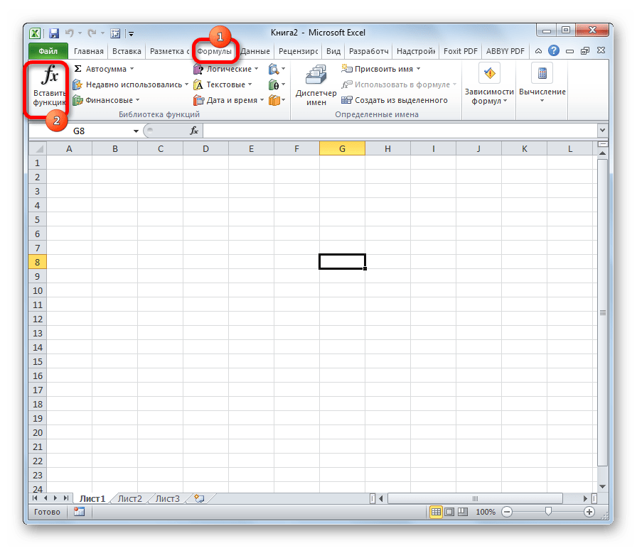
В Мастер функций также можно перейти через вкладку «Формулы». Сделав переход в неё, нужно нажать на кнопку на ленте «Вставить функцию», размещенную в блоке инструментов «Библиотека функций». Сразу вслед за этим запустится Мастер функций.

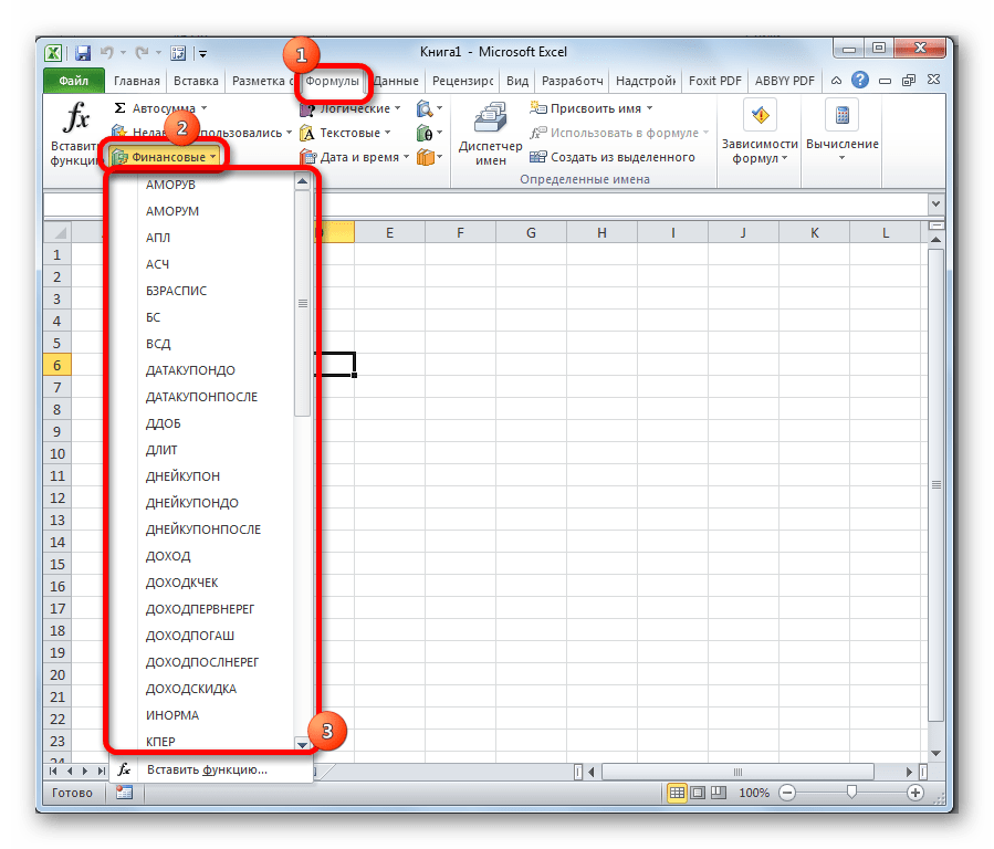
Имеется в наличии также способ перехода к нужному финансовому оператору без запуска начального окна Мастера. Для этих целей в той же вкладке «Формулы» в группе настроек «Библиотека функций» на ленте кликаем по кнопке «Финансовые». После этого откроется выпадающий список всех доступных инструментов данного блока. Выбираем нужный элемент и кликаем по нему. Сразу после этого откроется окно его аргументов.

Урок: Мастер функций в Excel

ДОХОД

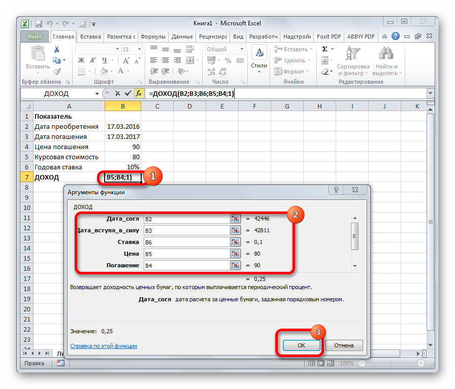
Одним из наиболее востребованных операторов у финансистов является функция ДОХОД. Она позволяет рассчитать доходность ценных бумаг по дате соглашения, дате вступления в силу (погашения), цене за 100 рублей выкупной стоимости, годовой процентной ставке, сумме погашения за 100 рублей выкупной стоимости и количеству выплат (частота). Именно эти параметры являются аргументами данной формулы. Кроме того, имеется необязательный аргумент «Базис». Все эти данные могут быть введены с клавиатуры прямо в соответствующие поля окна или храниться в ячейках листах Excel. В последнем случае вместо чисел и дат нужно вводить ссылки на эти ячейки. Также функцию можно ввести в строку формул или область на листе вручную без вызова окна аргументов. При этом нужно придерживаться следующего синтаксиса:

=ДОХОД(Дата_сог;Дата_вступ_в_силу;Ставка;Цена;Погашение»Частота;[Базис])

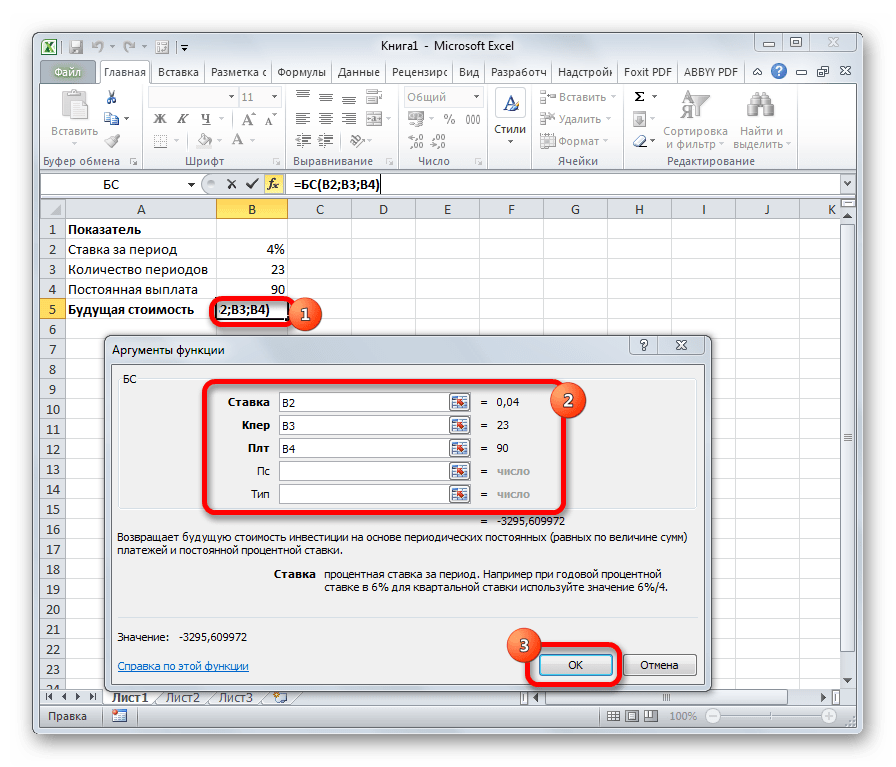
БС

Главной задачей функции БС является определение будущей стоимости инвестиций. Её аргументами является процентная ставка за период («Ставка»), общее количество периодов («Кол_пер») и постоянная выплата за каждый период («Плт»). К необязательным аргументам относится приведенная стоимость («Пс») и установка срока выплаты в начале или в конце периода («Тип»). Оператор имеет следующий синтаксис:

=БС(Ставка;Кол_пер;Плт;[Пс];[Тип])

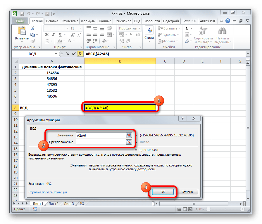
ВСД

Оператор ВСД вычисляет внутреннюю ставку доходности для потоков денежных средств. Единственный обязательный аргумент этой функции – это величины денежных потоков, которые на листе Excel можно представить диапазоном данных в ячейках («Значения»). Причем в первой ячейке диапазона должна быть указана сумма вложения со знаком «-», а в остальных суммы поступлений. Кроме того, есть необязательный аргумент «Предположение». В нем указывается предполагаемая сумма доходности. Если его не указывать, то по умолчанию данная величина принимается за 10%. Синтаксис формулы следующий:

=ВСД(Значения;[Предположения])

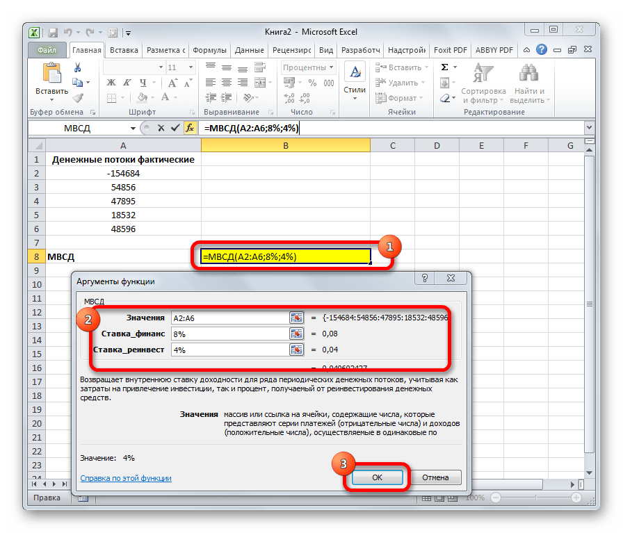
МВСД

Оператор МВСД выполняет расчет модифицированной внутренней ставки доходности, учитывая процент от реинвестирования средств. В данной функции кроме диапазона денежных потоков («Значения») аргументами выступают ставка финансирования и ставка реинвестирования. Соответственно, синтаксис имеет такой вид:

=МВСД(Значения;Ставка_финансир;Ставка_реинвестир)

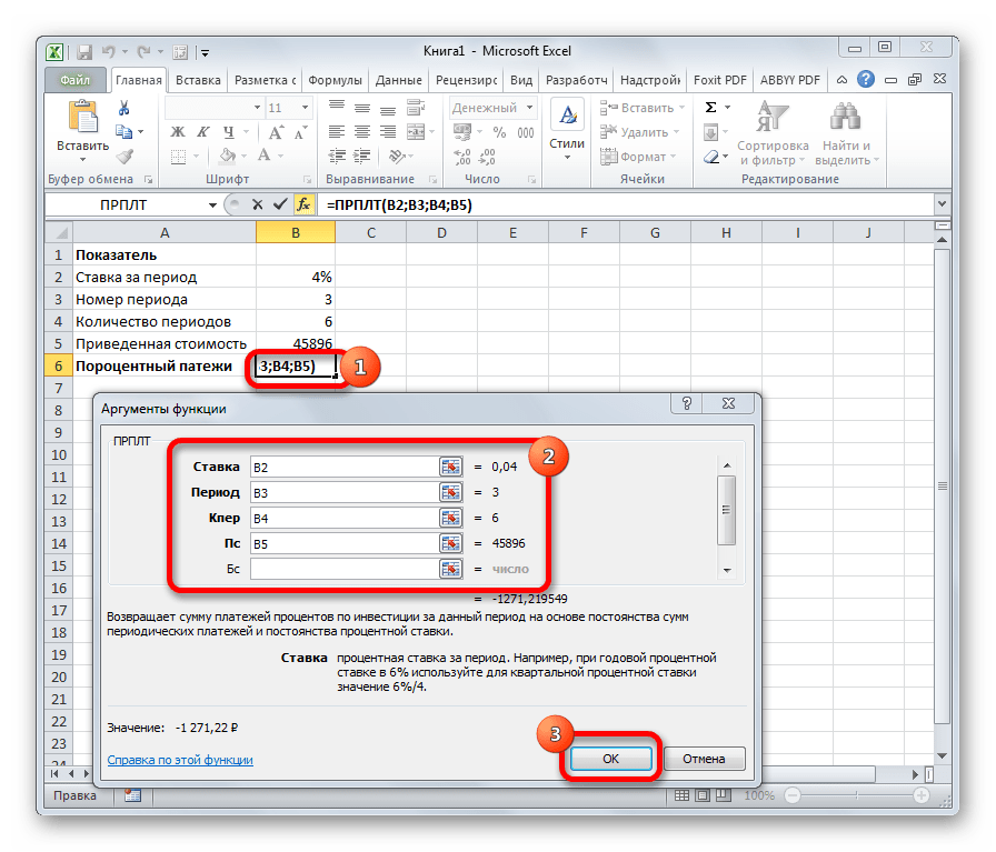
ПРПЛТ

Оператор ПРПЛТ рассчитывает сумму процентных платежей за указанный период. Аргументами функции выступает процентная ставка за период («Ставка»); номер периода («Период»), величина которого не может превышать общее число периодов; количество периодов («Кол_пер»); приведенная стоимость («Пс»). Кроме того, есть необязательный аргумент – будущая стоимость («Бс»). Данную формулу можно применять только в том случае, если платежи в каждом периоде осуществляются равными частями. Синтаксис её имеет следующую форму:

=ПРПЛТ(Ставка;Период;Кол_пер;Пс;[Бс])

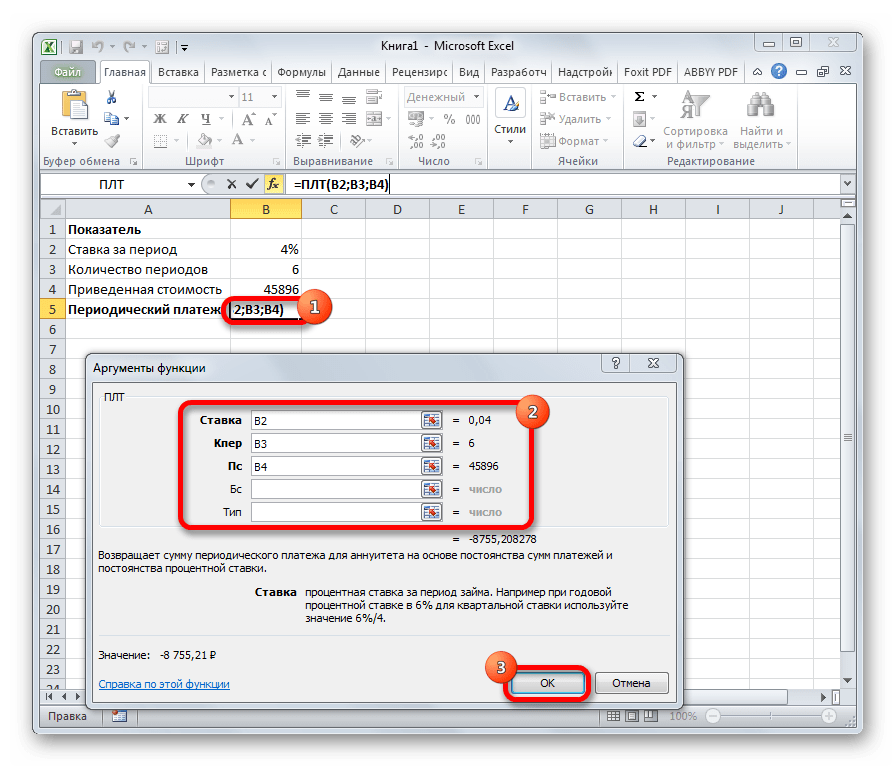
ПЛТ

Оператор ПЛТ рассчитывает сумму периодического платежа с постоянным процентом. В отличие от предыдущей функции, у этой нет аргумента «Период». Зато добавлен необязательный аргумент «Тип», в котором указывается в начале или в конце периода должна производиться выплата. Остальные параметры полностью совпадают с предыдущей формулой. Синтаксис выглядит следующим образом:

=ПЛТ(Ставка;Кол_пер;Пс;[Бс];[Тип])

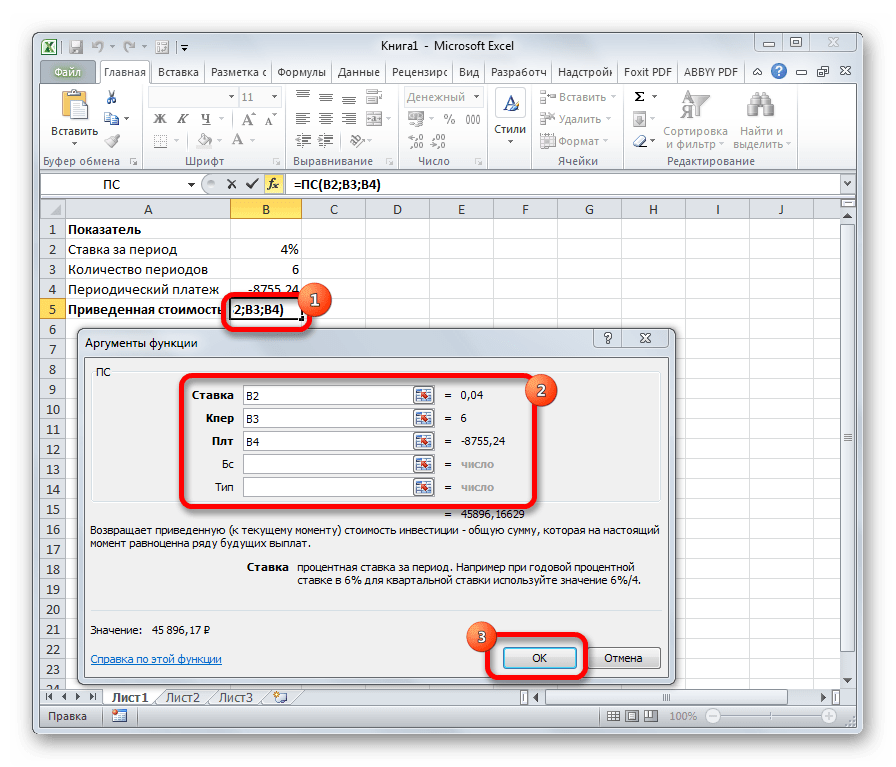
ПС

Формула ПС применяется для расчета приведенной стоимости инвестиции. Данная функция обратная оператору ПЛТ. У неё точно такие же аргументы, но только вместо аргумента приведенной стоимости («ПС»), которая собственно и рассчитывается, указывается сумма периодического платежа («Плт»). Синтаксис соответственно такой:

=ПС(Ставка;Кол_пер;Плт;[Бс];[Тип])

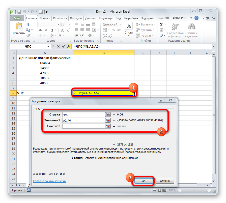
ЧПС

Следующий оператор применяется для вычисления чистой приведенной или дисконтированной стоимости. У данной функции два аргумента: ставка дисконтирования и значение выплат или поступлений. Правда, второй из них может иметь до 254 вариантов, представляющих денежные потоки. Синтаксис этой формулы такой:

=ЧПС(Ставка;Значение1;Значение2;…)

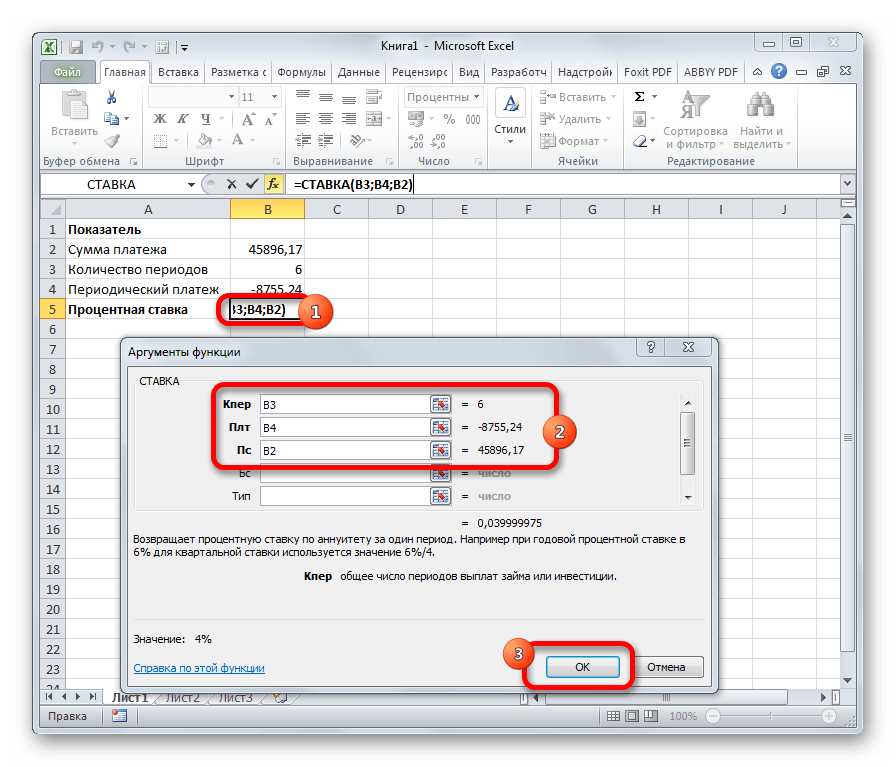
СТАВКА

Функция СТАВКА рассчитывает ставку процентов по аннуитету. Аргументами этого оператора является количество периодов («Кол_пер»), величина регулярной выплаты («Плт») и сумма платежа («Пс»). Кроме того, есть дополнительные необязательные аргументы: будущая стоимость («Бс») и указание в начале или в конце периода будет производиться платеж («Тип»). Синтаксис принимает такой вид:

=СТАВКА(Кол_пер;Плт;Пс[Бс];[Тип])

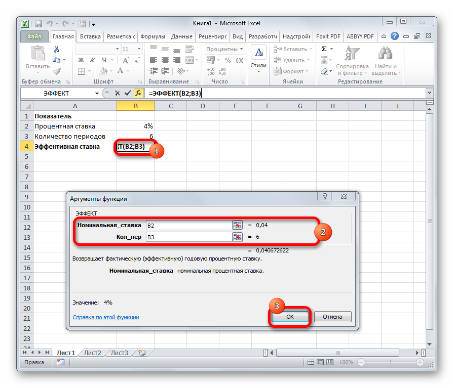
ЭФФЕКТ

Оператор ЭФФЕКТ ведет расчет фактической (или эффективной) процентной ставки. У этой функции всего два аргумента: количество периодов в году, для которых применяется начисление процентов, а также номинальная ставка. Синтаксис её выглядит так:

=ЭФФЕКТ(Ном_ставка;Кол_пер)

Нами были рассмотрены только самые востребованные финансовые функции. В общем, количество операторов из данной группы в несколько раз больше. Но и на данных примерах хорошо видна эффективность и простота применения этих инструментов, значительно облегчающих расчеты для пользователей.

Источник

Excel has many special financial functions. This guide shows how to solve time value of money problems using financial functions in Excel.

Time value of money (TVM) is the idea that money is worth more today than in the future. Time value of money is a foundational concept in finance.

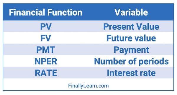
The following five functions are the basic Excel financial functions that everyone should know. These are also the five functions of a financial calculator.

Variable	Financial Functions	Description
Present Value	PV	lump sum at the beginning of a problem
Future value	FV	lump sum at the end of a problem
Payment	PMT	annuity, stream of equal payments per period (+ or -)
Number of periods	NPER	number of periods (months, quarters, half years, years)
Interest rate	RATE	interest rate per period (annual interest rate/periods per year)

Financial Functions in Excel

Present value (PV)

The PV function is a financial function that returns the present value of an investment. You can use the PV function to get the value in today’s dollars of a series of future payments, assuming periodic, constant payments and a constant interest rate.

=PV (rate, nper, pmt, [fv], [type])

rate – The interest rate per period.
nper – The total number of payment periods.
pmt – The payment made each period.
fv – [optional] A cash balance you want to attain after the last payment is made. If omitted, assumed to be zero.
type – [optional] When payments are due. 0 = end of period, 1 = beginning of period. Default is 0.

Future value (FV)

The FV function is a financial function that returns the future value of an investment. You can use the FV function to get the future value of an investment assuming periodic, constant payments with a constant interest rate.

=FV (rate, nper, pmt, [pv], [type])

rate – The interest rate per period.
nper – The total number of payment periods.
pmt – The payment made each period. Must be entered as a negative number.
pv – [optional] The present value of future payments. If omitted, assumed to be zero. Must be entered as a negative number.
type – [optional] When payments are due. 0 = end of period, 1 = beginning of period. Default is 0.

Payment (PMT)

The PMT function is a financial function that returns the periodic payment for a loan. You can use the NPER function to figure out payments for a loan, given the loan amount, number of periods, and interest rate.

=PMT (rate, nper, pv, [fv], [type])

rate – The interest rate for the loan.
nper – The total number of payments for the loan.
pv – The present value, or total value of all loan payments now.
fv – [optional] The future value, or a cash balance you want after the last payment is made. Defaults to 0 (zero).
type – [optional] When payments are due. 0 = end of period. 1 = beginning of period. Default is 0.

Excel Financial Functions

Number of periods (NPER)

The NPER function is a financial function that returns the number of periods for loan or investment. You can use the NPER function to get the number of payment periods for a loan, given the amount, the interest rate, and periodic payment amount.

=NPER (rate, pmt, pv, [fv], [type])

rate – The interest rate per period.
pmt – The payment made each period.
pv – The present value, or total value of all payments now.
fv – [optional] The future value, or a cash balance you want after the last payment is made. Defaults to 0.
type – [optional] When payments are due. 0 = end of period. 1 = beginning of period. Default is 0.

Interest rate (RATE)

The Excel RATE function is a financial function that returns the interest rate per period of an annuity. You can use RATE to calculate the periodic interest rate, then multiply as required to derive the annual interest rate. The RATE function calculates by iteration.

=RATE (nper, pmt, pv, [fv], [type], [guess])

nper – The total number of payment periods.
pmt – The payment made each period.
pv – The present value, or total value of all loan payments now.
fv – [optional] The future value, or desired cash balance after last payment. Default is 0.
type – [optional] When payments are due. 0 = end of period. 1 = beginning of period. Default is 0.
guess – [optional] Your guess on the rate. Default is 10%.

Using a financial calculator

The most popular financial calculator the TI BA II Plus Professional (Amazon affiliate link). This is the model that I recommend.

The BA II Plus Professional is the upgraded version of the TI BA II Plus (Amazon affiliate link). This calculator is used by many business students and professionals for calculating time value of money problems.

The BA II Plus and the BA II Plus Professional are official calculators for the following professional exams:

Chartered Financial Analyst (CFA)

Certified Financial Planner (CFP)

Certified Management Accountant (CMA)

Excel vs. financial calculator

Excel and the TI BA II Plus are both excellent at calculating TVM problems. They do have slightly different function names. The following table summarizes the differences.

Variable	Excel	TI BA II Plus
Periods per Year	–	P/Y
Number of Periods	NPER	N
Interest Rate	RATE	I/Y
Present Value	PV	PV
Payment	PMT	PMT
Future Value	FV	FV

Excel Financial Functions vs. TI BA II Plus

Time value of money using Excel financial functions

Time value of money using BA II Plus

Advanced Excel financial functions

Excel can also perform several advanced financial functions. The following table summarizes these functions.

Financial Functions	Meaning
NPV	net present value
IRR	internal rate of return
CUMIPMT	cumulative interest
CUMPRINC	cumulative principal
FVSCHEDULE	future value schedule

Net present value (NPV)

The Excel NPV function calculates the Net Present Value of an investment, based on a supplied discount rate, and a series of future payments and income.

=NPV (rate, value1, value2,…)

rate – is the rate of discount over the length of one period.
value1 – value1,value2,… are 1 to 254 payments and income, equally spaced in time and occurring at the end of each period.
value2 – 1value1,value2,… are 1 to 254 payments and income, equally spaced in time and occurring at the end of each period.

Internal rate of return (IRR)

The Excel IRR function returns the Internal Rate of Return for a supplied series of periodic cash flows (i.e. an initial investment value and a series of net income values).

=IRR (values, guess)

Values – is an array or a reference to cells that contain numbers for which you want to calculate the internal rate of return.
Guess – is a number that you guess is close to the result of IRR; 0.1 (10 percent) if omitted.

Cumulative interest payment (CUMIPMT)

The Excel CUMIPMT function is a financial function that returns the cumulative interest paid on a loan between a start period and an end period. You can use CUMIPMT to calculate and verify the total interest paid on a loan, or the interest paid between any two payment periods.

=CUMIPMT (rate, nper, pv, start_period, end_period, type)

rate – The interest rate per period.
nper – The total number of payments for the loan.
pv – The present value, or total value of all payments now.
start_period – First payment in calculation.
end_period – Last payment in calculation.
type – When payments are due. 0 = end of period. 1 = beginning of period.

Cumulative principal (CUMPRINC)

The Excel CUMPRINC function is a financial function that returns the cumulative principal paid on a loan between a start period and an end period. You can use CUMPRINC to calculate and verify the total principal paid on a loan, or the principal paid between any two payment periods.

=CUMPRINC (rate, nper, pv, start_period, end_period, type)

Future value schedule (FVSCHEDULE)

Returns the future value of an initial principal after applying a series of compound interest rates.

=FVSCHEDULE(principal,schedule)

Principal – is the present value.
Schedule – is an array of interest rates to apply.

Video: Top 15 financial functions in Excel

Источник

Table of contents

#1 – Future Value (FV): Financial Function in Excel

FV Example

#2 – FVSCHEDULE: Financial Function in Excel

FVSCHEDULE Example:

#3 – Present Value (PV): Financial Function in Excel

PV Example:

#4 – Net Present Value (NPV): Financial Function in Excel

NPV Example

#5 – XNPV: Financial Function in Excel

XNPV Example

#6 – PMT: Financial Function in Excel

PMT Example

#7 – PPMT: Financial Function in Excel

PPMT Example

#8 – Internal Rate of Return (IRR): Financial Function in Excel

IRR Example

#9 – Modified Internal Rate of Return (MIRR): Financial Function in Excel

MIRR Example

#10 – XIRR: Financial Function in Excel

XIRR Example

#11 – NPER: Financial Function in Excel

NPER Example

#12 – RATE: Financial Function in Excel

RATE Example

#13 – EFFECT: Financial Function in Excel

EFFECT Example

#14 – NOMINAL: Financial Function in Excel

NOMINAL Example

#15 – SLN: Financial Function in Excel

SLN Example

Top 15 Financial Functions in Excel Video

Recommended Articles

1. FV Function

Syntax

Arguments

Notes

Example

2. PMT

Syntax

Arguments

Notes

Example

3. PV

Syntax

Arguments

Notes

Example

More Excel Tutorials

Выполнение расчетов с помощью финансовых функций

ДОХОД

БС

ВСД

МВСД

ПРПЛТ

ПЛТ

ПС

ЧПС

СТАВКА

ЭФФЕКТ

Present value (PV)

Future value (FV)

Payment (PMT)

Number of periods (NPER)

Interest rate (RATE)

Using a financial calculator

Excel vs. financial calculator

Time value of money using Excel financial functions

Time value of money using BA II Plus

Advanced Excel financial functions

Net present value (NPV)

Internal rate of return (IRR)

Cumulative interest payment (CUMIPMT)

Cumulative principal (CUMPRINC)

Future value schedule (FVSCHEDULE)

Video: Top 15 financial functions in Excel