
Excel for Microsoft 365 Excel for Microsoft 365 for Mac Excel 2021 Excel 2021 for Mac Excel 2019 Excel 2019 for Mac Excel 2016 Excel 2016 for Mac Excel 2013 Excel 2010 Excel 2007 Excel for Mac 2011 More…Less
By using What-If Analysis tools in Excel, you can use several different sets of values in one or more formulas to explore all the various results.
For example, you can do What-If Analysis to build two budgets that each assumes a certain level of revenue. Or, you can specify a result that you want a formula to produce, and then determine what sets of values will produce that result. Excel provides several different tools to help you perform the type of analysis that fits your needs.
Note that this is just an overview of those tools. There are links to help topics for each one specifically.
What-If Analysis is the process of changing the values in cells to see how those changes will affect the outcome of formulas on the worksheet.
Three kinds of What-If Analysis tools come with Excel: Scenarios, Goal Seek, and Data Tables. Scenarios and Data tables take sets of input values and determine possible results. A Data Table works with only one or two variables, but it can accept many different values for those variables. A Scenario can have multiple variables, but it can only accommodate up to 32 values. Goal Seek works differently from Scenarios and Data Tables in that it takes a result and determines possible input values that produce that result.
In addition to these three tools, you can install add-ins that help you perform What-If Analysis, such as the Solver add-in. The Solver add-in is similar to Goal Seek, but it can accommodate more variables. You can also create forecasts by using the fill handle and various commands that are built into Excel.
For more advanced models, you can use the Analysis ToolPak add-in.
A Scenario is a set of values that Excel saves and can substitute automatically in cells on a worksheet. You can create and save different groups of values on a worksheet and then switch to any of these new scenarios to view different results.
For example, suppose you have two budget scenarios: a worst case and a best case. You can use the Scenario Manager to create both scenarios on the same worksheet, and then switch between them. For each scenario, you specify the cells that change and the values to use for that scenario. When you switch between scenarios, the result cell changes to reflect the different changing cell values.
1. Changing cells
2. Result cell
1. Changing cells
2. Result cell
If several people have specific information in separate workbooks that you want to use in scenarios, you can collect those workbooks and merge their scenarios.
After you have created or gathered all the scenarios that you need, you can create a Scenario Summary Report that incorporates information from those scenarios. A scenario report displays all the scenario information in one table on a new worksheet.
Note: Scenario reports are not automatically recalculated. If you change the values of a scenario, those changes will not show up in an existing summary report. Instead, you must create a new summary report.
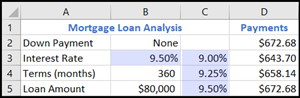
If you know the result that you want from a formula, but you’re not sure what input value the formula requires to get that result, you can use the Goal Seek feature. For example, suppose that you need to borrow some money. You know how much money you want, how long a period you want in which to pay off the loan, and how much you can afford to pay each month. You can use Goal Seek to determine what interest rate you must secure in order to meet your loan goal.

Cells B1, B2, and B3 are the values for the loan amount, term length, and interest rate.
Cell B4 displays the result of the formula =PMT(B3/12,B2,B1).
Note: Goal Seek works with only one variable input value. If you want to determine more than one input value, for example, the loan amount and the monthly payment amount for a loan, you should instead use the Solver add-in. For more information about the Solver add-in, see the section Prepare forecasts and advanced business models, and follow the links in the See Also section.
If you have a formula that uses one or two variables, or multiple formulas that all use one common variable, you can use a Data Table to see all the outcomes in one place. Using Data Tables makes it easy to examine a range of possibilities at a glance. Because you focus on only one or two variables, results are easy to read and share in tabular form. If automatic recalculation is enabled for the workbook, the data in Data Tables immediately recalculates; as a result, you always have fresh data.
Cell B3 contains the input value.
Cells C3, C4, and C5 are values Excel substitutes based on the value entered in B3.
A Data Table cannot accommodate more than two variables. If you want to analyze more than two variables, you can use Scenarios. Although it is limited to only one or two variables, a Data Table can use as many different variable values as you want. A Scenario can have a maximum of 32 different values, but you can create as many scenarios as you want.
If you want to prepare forecasts, you can use Excel to automatically generate future values that are based on existing data, or to automatically generate extrapolated values that are based on linear trend or growth trend calculations.
You can fill in a series of values that fit a simple linear trend or an exponential growth trend by using the fill handle or the Series command. To extend complex and nonlinear data, you can use worksheet functions or the regression analysis tool in the Analysis ToolPak Add-in.
Although Goal Seek can accommodate only one variable, you can project backward for more variables by using the Solver add-in. By using Solver, you can find an optimal value for a formula in one cell—called the target cell—on a worksheet.
Solver works with a group of cells that are related to the formula in the target cell. Solver adjusts the values in the changing cells that you specify—called the adjustable cells—to produce the result that you specify from the target cell formula. You can apply constraints to restrict the values that Solver can use in the model, and the constraints can refer to other cells that affect the target cell formula.
Need more help?
You can always ask an expert in the Excel Tech Community or get support in the Answers community.
See Also
Scenarios
Goal Seek
Data Tables
Using Solver for capital budgeting
Using Solver to determine the optimal product mix
Define and solve a problem by using Solver
Analysis ToolPak Add-in
Overview of formulas in Excel
How to avoid broken formulas
Detect errors in formulas
Keyboard shortcuts in Excel
Excel functions (alphabetical)
Excel functions (by category)
Need more help?
Чтобы проанализировать изменчивость признака под воздействием контролируемых переменных, применяется дисперсионный метод.
Для изучения связи между значениями – факторный метод. Рассмотрим подробнее аналитические инструменты: факторный, дисперсионный и двухфакторный дисперсионный метод оценки изменчивости.
Дисперсионный анализ в Excel
Условно цель дисперсионного метода можно сформулировать так: вычленить из общей вариативности параметра 3 частные вариативности:
- 1 – определенную действием каждого из изучаемых значений;
- 2 – продиктованную взаимосвязью между исследуемыми значениями;
- 3 – случайную, продиктованную всеми неучтенными обстоятельствами.
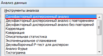
В программе Microsoft Excel дисперсионный анализ можно выполнить с помощью инструмента «Анализ данных» (вкладка «Данные» — «Анализ»). Это надстройка табличного процессора. Если надстройка недоступна, нужно открыть «Параметры Excel» и включить настройку для анализа.
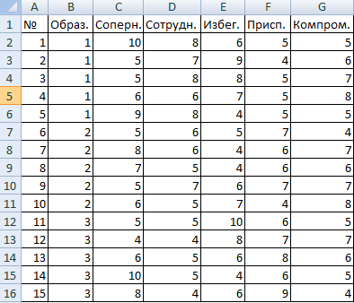
Работа начинается с оформления таблицы. Правила:
- В каждом столбце должны быть значения одного исследуемого фактора.
- Столбцы расположить по возрастанию/убыванию величины исследуемого параметра.
Рассмотрим дисперсионный анализ в Excel на примере.
Психолог фирмы проанализировал с помощью специальной методики стратегии поведения сотрудников в конфликтной ситуации. Предполагается, что на поведение влияет уровень образования (1 – среднее, 2 – среднее специальное, 3 – высшее).
Внесем данные в таблицу Excel:
- Открываем диалоговое окно нашего аналитического инструмента. В раскрывшемся списке выбираем «Однофакторный дисперсионный анализ» и нажимаем ОК.
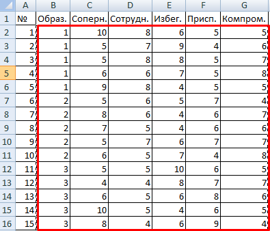
- В поле «Входной интервал» ввести ссылку на диапазон ячеек, содержащихся во всех столбцах таблицы.
- «Группирование» назначить по столбцам.
- «Параметры вывода» — новый рабочий лист. Если нужно указать выходной диапазон на имеющемся листе, то переключатель ставим в положение «Выходной интервал» и ссылаемся на левую верхнюю ячейку диапазона для выводимых данных. Размеры определятся автоматически.
- Результаты анализа выводятся на отдельный лист (в нашем примере).
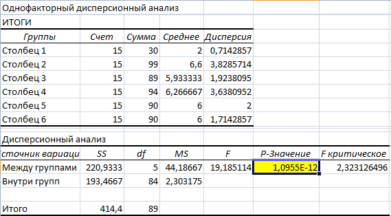
Значимый параметр залит желтым цветом. Так как Р-Значение между группами больше 1, критерий Фишера нельзя считать значимым. Следовательно, поведение в конфликтной ситуации не зависит от уровня образования.
Факторный анализ в Excel: пример
Факторным называют многомерный анализ взаимосвязей между значениями переменных. С помощью данного метода можно решить важнейшие задачи:
- всесторонне описать измеряемый объект (причем емко, компактно);
- выявить скрытые переменные значения, определяющие наличие линейных статистических корреляций;
- классифицировать переменные (определить взаимосвязи между ними);
- сократить число необходимых переменных.
Рассмотрим на примере проведение факторного анализа. Допустим, нам известны продажи каких-либо товаров за последние 4 месяца. Необходимо проанализировать, какие наименования пользуются спросом, а какие нет.
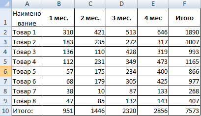
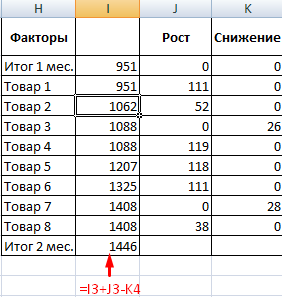
- Посмотрим, за счет, каких наименований произошел основной рост по итогам второго месяца. Если продажи какого-то товара выросли, положительная дельта – в столбец «Рост». Отрицательная – «Снижение». Формула в Excel для «роста»: =ЕСЛИ((C2-B2)>0;C2-B2;0), где С2-В2 – разница между 2 и 1 месяцем. Формула для «снижения»: =ЕСЛИ(J3=0;B2-C2;0), где J3 – ссылка на ячейку слева («Рост»). Во втором столбце – сумма предыдущего значения и предыдущего роста за вычетом текущего снижения.
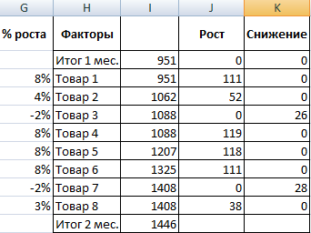
- Рассчитаем процент роста по каждому наименованию товара. Формула: =ЕСЛИ(J3/$I$11=0;-K3/$I$11;J3/$I$11). Где J3/$I$11 – отношение «роста» к итогу за 2 месяц, ;-K3/$I$11 – отношение «снижения» к итогу за 2 месяц.
- Выделяем область данных для построения диаграммы. Переходим на вкладку «Вставка» — «Гистограмма».
- Поработаем с подписями и цветами. Уберем накопительный итог через «Формат ряда данных» — «Заливка» («Нет заливки»). С помощью данного инструментария меняем цвет для «снижения» и «роста».
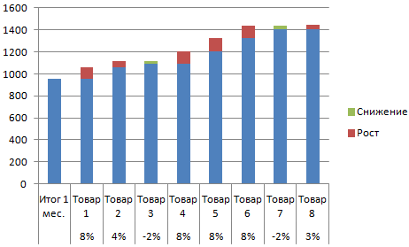
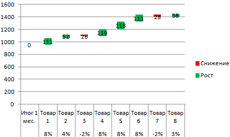
Теперь наглядно видно, продажи какого товара дают основной рост.
Двухфакторный дисперсионный анализ в Excel
Показывает, как влияет два фактора на изменение значения случайной величины. Рассмотрим двухфакторный дисперсионный анализ в Excel на примере.
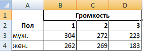
Задача. Группе мужчин и женщин предъявляли звук разной громкости: 1 – 10 дБ, 2 – 30 дБ, 3 – 50 дБ. Время ответа фиксировали в миллисекундах. Необходимо определить, влияет ли пол на реакцию; влияет ли громкость на реакцию.
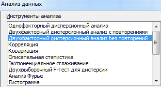
- Переходим на вкладку «Данные» — «Анализ данных» Выбираем из списка «Двухфакторный дисперсионный анализ без повторений».
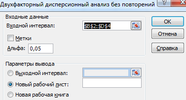
- Заполняем поля. В диапазон должны войти только числовые значения.
- Результат анализа выводится на новый лист (как было задано).
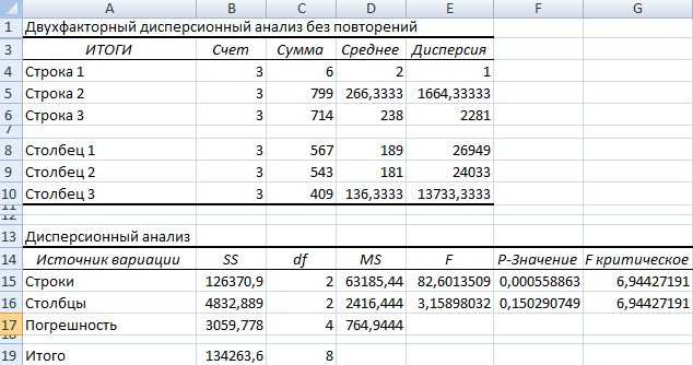
Та как F-статистики (столбец «F») для фактора «Пол» больше критического уровня F-распределения (столбец «F-критическое»), данный фактор имеет влияние на анализируемый параметр (время реакции на звук).
Скачать пример факторного и дисперсионного анализа
скачать факторный анализ отклонений
скачать пример 2
Для фактора «Громкость»: 3,16 < 6,94. Следовательно, данный фактор не влияет на время ответа.
Для примера также прилагаем факторный анализ отклонений в маржинальном доходе.
What-if analysis is the option available in Data. In what-if analysis, by changing the input value in some cells you can see the effect on output. It tells about the relationship between input values and output values. In this article, we will learn how to use the what-if analysis with data tables effectively.
What is What-if Analysis?
What-if analysis is a procedure in excel in which we work in tabular form data. In the What-if analysis variety of values have been in the cell of the excel sheet to see the result in different ways by not creating different sheets. There are three tools of what-if analysis.
Tools of what-if analysis
There are three tools in what-if analysis:
- Goal seek
- Scenario manager
- Data Table
Goal seek
In goal seek we already know our output value we have to find the correct input value. For example, if a student wants to know his English marks and he knows all the rest of the marks and total marks in all subjects.
Step 1: Write all subjects and their marks in an excel sheet and do the sum by applying the formula sum.
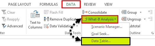
Step 2: Go into the data tab of the Toolbar.
Step 3: Under the Data Table section, Select the What-if analysis.
Step 4: A drop-down appears. Select the Goal Seek.
Step 5: The dialogue box appears in the first column write the name of the cell in which you apply the formula sum. Type D10 in Set cell.
Step 6: In the second column write the value of the target. The target value for this example is 440.
Step 7: In the third column write the name of the cell in which you want to get marks in English. Provide absolute cell reference, i.e. $D$5.
Step 8: Click ok and see the result. The estimated marks for English are 71.
Scenario Manager
In scenario manager, we create different scenarios by proving different input values for the same variable than by comparing scenarios to choose the correct result. For Example, To check the cost of revenue for three different months.
Step 1: Given a data set, for Revenue Cost of Jan, with Expenses and Cost as its columns.
Step 2: Select the numerical value cell and Go to the Data.
Step 3: Under the forecast section, click on the What-if analysis.
Step 4: A drop-down appears. Select the Scenario manager.
Step 5: A dialog box appears in the dialog box select add option.
Step 6: A new dialog appears to write the name of the new scenario in the first column. Under Scenario name, write “Revenue of Feb”.
Step 7: In the second column select the changing cell. The changing cells for this example, are $E$5:$E$9.
Step 8: A new dialogue box name Scenario Values appears to write the changed value in the box. Enter the values as per shown in the image. Click Ok.
Step 9: Repeat step5, step6, and step8.
Step 10: Click Ok then select summary.
Step 11: A new Dialog box name Scenario Summary appears. Select Result cells: $E$10.
Step 12: See the result.
Data Table
In data, we create a table with different input values for the same variables. It is one of the most helpful features in what-if analysis. One can change different values in x and can achieve different outputs accordingly for research as well as business-driven purposes.
A data table is of two types:
Data table in one Variable
In the data table in one variable, we can change only one input value either in a row or in a column. It includes only one input cell. For example, a company wants to know about its revenue by changing the cost of raw materials by using a data table. Given a data set, with material and their cost.
Step 1: Create a table of revenue cost.
Step 2: Copy the last cell in which you get output in another cell. D7 for this example.
Step 3: Write the values in the cell for which you want to make a change in a column or in rows.
Step 4: Go to the data tab of the Toolbar.
Step 5: Under the data table section, Select the what-if analysis.
Step 6: A drop-down appears. Select the Data Table.
Step 7: A dialogue box name data table appears then select the cell in which you want to change the input value in a row or in the column. Input the value of the Column input cell to be $D$3. Click Ok. Your data table is ready.
Data table in two Variable
In the Data table in two variables, we can change two input values in both row and column. It includes two input cells. For example, A person wants to know about per month installments of loan by the different rates of interest and for the different time periods for the same principal amount.
Step 1: Create a table to find PMT.
Step 2: Copy the last cell in which you get output in another cell
Step 3: Write both values you want to change in both columns and rows.
Step 4: Go to the Data tab of the toolbar.
Step 5: Select the what-if analysis.
Step 6: Select the Data Table.
Step 7: A dialogue box appears in which you have to select the cell in which you want to change the value in both row and column. The Row input cell value is $D$5 and the column input cell value is $D$6.
Step 8: Click ok and see the result.
Excel’s What-If Analysis Scenario Manager helps you compare multiple data sets and decide based on data analysis.

Excel has many powerful tools, including the What-If Analysis, which helps you perform different types of mathematical calculations. It allows you to experiment with different formula parameters to explore the effects of variations in the result.
So, instead of dealing with complex mathematical calculations to get the answers you seek, you can simply use the What-If Analysis in Excel.
When Is What-If Analysis Used?
You should use the What-If Analysis if you would like to see how a change of value in your cells will affect the outcome of the formulas in your worksheet.
Excel provides different tools that will help you perform all sorts of analyses that fit your needs. So it all comes down to what you want.
For example, you can use the What-If Analysis if you want to build two budgets, both of which will require a certain level of revenue. With this tool, you could also determine what sets of values you need in order to produce a certain result.

There are three kinds of What-If Analysis tools that you have in Excel: Goal Seek, Scenarios, and Data Tables.
Goal Seek
When you create a function or a formula in Excel, you put different parts together to get appropriate results. However, Goal Seek works oppositely, as you get to start with the result you want.
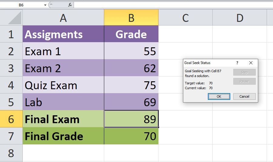
Goal Seek is most often used if you want to know the value that you need to get a certain result. For example, if you want to calculate the grade, you would need to get in school in order for you to pass the class.
A simple example would look like this. If you would like your final grade to have an average of 70 points, you first need to calculate your overall average, including the empty cell.
You can do that with this function:
<strong>=AVERAGE(B2:B6)</strong>
Once you know your average, you should go to Data > What-If Analysis > Goal Seek. Then calculate the Goal Seek using the information that you have. In this case, that would be:
If you want to learn more about it, you can check out our following guide on Goal Seek.
Scenarios
In Excel, Scenarios allow you to substitute values for multiple cells simultaneously (up to 32). You can create many Scenarios and compare them without having to change the values manually.
For example, if you have the worst and the best-case scenarios, you can use the Scenario Manager in Excel to create both of these scenarios.
In both scenarios, you need to specify the cells that change values, and the values that might be used for that scenario. You can find a good example of this on Microsoft’s website.
Data Tables
Unlike Goal Seek or Scenarios, this option allows you to see multiple results simultaneously. You can replace one or two variables in a formula with as many different values as you like and then see the results in a table.
This makes it easy to examine a range of possibilities with just one glance. However, a Data Table cannot accommodate more than 2 variables. If that is what you were hoping for, you should use Scenarios instead.

Visualize Your Data With What-If Analysis in Excel
If you use Excel frequently, you will discover many formulas and functions that make life easier. The What-If Analysis is just one of many examples that can simplify your most complex mathematical calculations.
With the What-If Analysis in Excel, you get to experiment with different answers to the same question, even if your data is incomplete. To get the most out of the What-If Analysis, you should be fairly comfortable with functions and formulas in Excel.
What-If Analysis in Excel is a tool that helps us create different models, scenarios, and Data Tables. This article will look at the ways of using What-If Analysis.
Table of contents
- What is a What-If Analysis in Excel?
- #1 Scenario Manager in What-If Analysis
- #2 Goal Seek in What-If Analysis
- #3 Data Table in What-If Analysis
- Things to Remember
- Recommended Articles
We have three parts of What-If Analysis in Excel. They are as follows:
- Scenario Manager
- Goal Seek in Excel
- Data Table in Excel
You can download this What-If Analysis Excel Template here – What-If Analysis Excel Template
#1 Scenario Manager in What-If Analysis
As a business head, it is important to know the different scenarios of your future project. Based on the scenarios, the business head will make decisions. For example, you are going to undertake one of the important projects. You have done your homework and listed all the possible expenditures from your end, and below is the list of all your expenses.
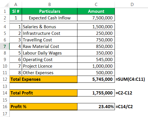
The expected cash flow from this project is $75 million, which is in cell C2. Total expenses comprise all your fixed and variable expenses, the total cost is $57.45 million in cell C12. Total profit is $17.55 million in cell C14, and profit % is 23.40% of your cash inflow.
It is the basic scenario of your project. Now, you need to know the profit scenario if some of your expenses increase or decrease.
Scenario 1
- In a general case scenario, you have estimated the “Project License” cost to be $10 million, but you are sure anticipating it to be $15 million
- Raw material costs to be increased by $2.5 million
- Other expensesOther expenses comprise all the non-operating costs incurred for the supporting business operations. Such payments like rent, insurance and taxes have no direct connection with the mainstream business activities.read more to be decreased by 50 thousand.
Scenario 2
- The “Project Cost” to be at $20 million
- The “Labor Daily Wages” to be at $5 million
- The “Operating Cost” is to be at $3.5 million
Now, you have listed out all the scenarios in the form. Based on these scenarios, you need to create a table about how it will impact your profit and profit %.
To create What-If Analysis scenarios, follow the below steps.
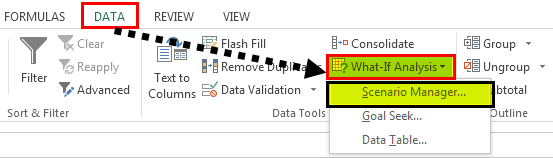
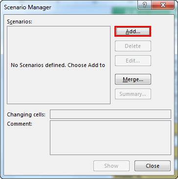
- Go to DATA > What-If Analysis > Scenario Manager.

- Once you click “Scenario Manager,” it will show you below the dialog box.

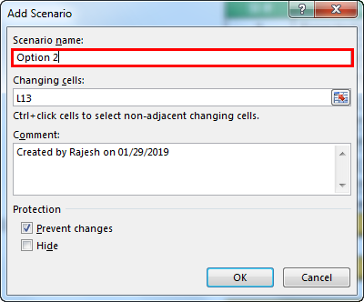
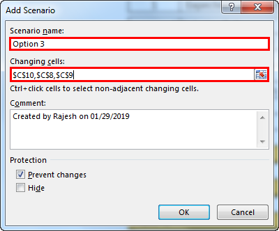
- Click on “Add.” Then, give “Scenario name.”

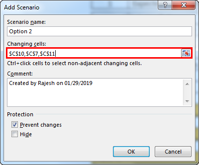
- In changing cells, select the first scenario changes you have listed out. The changes are Project License (cell C10) at $15 million, Raw Material Cost (cell C7) at $11 million, and Other Expenses (cell C11) at $4.5 million. Mention these three cells here.
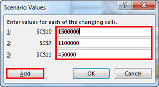
- Click on “OK.” It will ask you to mention the new values as listed in scenario 1.

- Do not click on “OK” but click on “OK Add.” It will save this scenario for you.
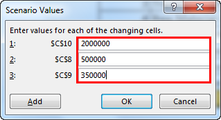
- Now, it will ask you to create one more scenario. As we listed in scenario 2, make the changes. This time we need to change Project Cost (C10), Labour Cost (C8), and Operating Cost (C9).
- Now, add new values here.
- Now click on “OK.” It will show all the scenarios we have created.
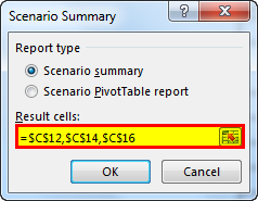
- Click on “Scenario summary.” It will ask you which result cells you want to change. Here, we need to change the Total Expense Cell (C12), Total Profit Cell (C14), and Profit % cell (C16).

- Click on “OK.” It will create a summary report for you in the new worksheet.


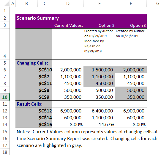
Total Excel has created three scenarios even though we have supplied only two scenario changes because Excel will show existing reports as one scenario.
From this table, we can easily see the impact of changes in pour profit %.
#2 Goal Seek in What-If Analysis
Now, we know the Scenario Manager’s advantage. What-if-Analysis Goal Seek can tell you what you must do to achieve the target.
Andrew is a class 10th student. His target is to achieve an average score of 85 in the final exam. He has already completed 5 exams and left with only 1 exam. Therefore, in the completed 5 exams.
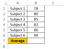
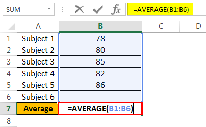
To calculate the current average, apply the average formula in the B7 cell.
The current average is 82.2.
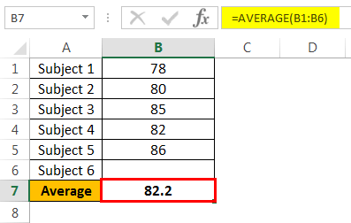
Andrew’s GOAL is 85. His current average is 82.2. He is short by 3.8 with one exam.
Now, the question is how much he has to score in the final exam to eventually get an overall average of 85. It can be found by the What-If Analysis GOAL SEEK tool.
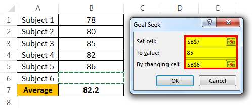
- Step 1: Go to DATA > What-If Analysis > Goal Seek.

- Step 2: It will show you below the dialog box.
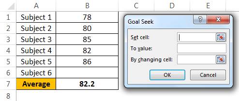
- Step 3: Here, we need to set the cell first. “Set cell” is nothing but which cell we need for the final result, i.e., our overall average cell (B7). Next is “To value.” Again, Andrew’s overall average GOAL is nothing but for what value we need to set the cell (85).
The next and final step is changing which cell you want to see the impact on. So, we need to change cell B6, the cell for the final subject’s score.
- Step 4: Click on “OK.” Excel will take a few seconds to complete the process, but it eventually shows the result like the one below.
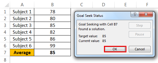
Now, we have our results here. To get an overall average of 85, Andrew has to score 99 in the final exam.
#3 Data Table in What-If Analysis
We have already seen two wonderful techniques under What-If Analysis in Excel. First, the Data Table can create different scenario tables based on the variable change. We have two kinds of Data Tables here: one variable Data Table and a “Two-variable data tableA two-variable data table helps analyze how two different variables impact the overall data table. In simple terms, it helps determine what effect does changing the two variables have on the result.read more.” This article will show you One variable data table in ExcelOne variable data table in excel means changing one variable with multiple options and getting the results for multiple scenarios. The data inputs in one variable data table are either in a single column or across a row.read more.
Assume you are selling 1,000 products at ₹15, your total anticipated expense is ₹12,500, and your profit is ₹2,500.
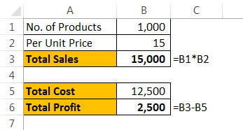
You are not happy with the profit you are getting. Your anticipated profit is ₹7,500. You have decided to increase your per-unit price to increase your profit, but you do not know how much you need to increase.
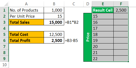
Data tables can help you. Create a table below.

Now, in the cell, F1 links to the “Total Profit” cell, B6.

- Step 1: Select the newly created table.
- Step 2: Go to DATA > What-if Analysis > Data Table.
- Step 3: Now, you will see below dialog box.
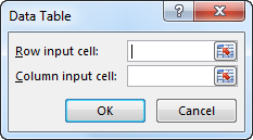
- Step 4: Since we are showing the result vertically, leave the ”Row input cell.” In the “Column input cell,” select cell B2, which is the original selling price.
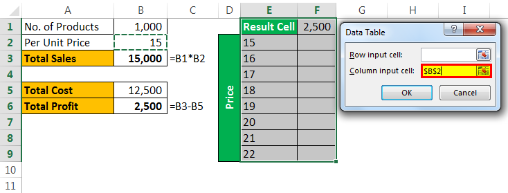
- Step 5: Click on “OK” to get the results. It will list out profit numbers in the new table.
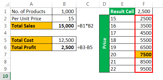
So, we have our Data Table ready. To profit from ₹7,500, you need to sell at ₹20 per unit.
Things to Remember
- The What-If Analysis data table can be performed with two variable changes. Refer to our article on What-If Analysis two-variable Data Table.
- What-If Analysis Goal Seek takes a few seconds to perform calculations.
- What-If Analysis Scenario Manager can give a summary with input numbers and current values together.
Recommended Articles
This article is a guide to What-If Analysis in Excel. Here, we discuss three types of What-If Analysis in Excel such as 1) Scenario Manager, 2) Goal Seek, 3) Data Tables along with practical examples, and a downloadable Excel template. You may learn more about Excel from the following articles: –
- Pareto Analysis in ExcelA pareto chart is a graph which is a combination of a bar graph and a line graph, indicates the defect frequency and its cumulative impact. It helps in finding the defects to observe the best possible and overall improvement measure.read more
- Goal Seek in VBA
- Sensitivity Analysis in Excel
Create Different Scenarios | Scenario Summary | Goal Seek
What-If Analysis in Excel allows you to try out different values (scenarios) for formulas. The following example helps you master what-if analysis quickly and easily.
Assume you own a book store and have 100 books in storage. You sell a certain % for the highest price of $50 and a certain % for the lower price of $20.

If you sell 60% for the highest price, cell D10 calculates a total profit of 60 * $50 + 40 * $20 = $3800.
Create Different Scenarios
But what if you sell 70% for the highest price? And what if you sell 80% for the highest price? Or 90%, or even 100%? Each different percentage is a different scenario. You can use the Scenario Manager to create these scenarios.
Note: You can simply type in a different percentage into cell C4 to see the corresponding result of a scenario in cell D10. However, what-if analysis enables you to easily compare the results of different scenarios. Read on.
1. On the Data tab, in the Forecast group, click What-If Analysis.

2. Click Scenario Manager.

The Scenario Manager dialog box appears.
3. Add a scenario by clicking on Add.

4. Type a name (60% highest), select cell C4 (% sold for the highest price) for the Changing cells and click on OK.

5. Enter the corresponding value 0.6 and click on OK again.

6. Next, add 4 other scenarios (70%, 80%, 90% and 100%).
Finally, your Scenario Manager should be consistent with the picture below:

Note: to see the result of a scenario, select the scenario and click on the Show button. Excel will change the value of cell C4 accordingly for you to see the corresponding result on the sheet.
Scenario Summary
To easily compare the results of these scenarios, execute the following steps.
1. Click the Summary button in the Scenario Manager.
2. Next, select cell D10 (total profit) for the result cell and click on OK.

Result:

Conclusion: if you sell 70% for the highest price, you obtain a total profit of $4100, if you sell 80% for the highest price, you obtain a total profit of $4400, etc. That’s how easy what-if analysis in Excel can be.
Goal Seek
What if you want to know how many books you need to sell for the highest price, to obtain a total profit of exactly $4700? You can use Excel’s Goal Seek feature to find the answer.
1. On the Data tab, in the Forecast group, click What-If Analysis.
2. Click Goal Seek.

The Goal Seek dialog box appears.
3. Select cell D10.
4. Click in the ‘To value’ box and type 4700.
5. Click in the ‘By changing cell’ box and select cell C4.
6. Click OK.

Result. You need to sell 90% of the books for the highest price to obtain a total profit of exactly $4700.

Note: visit our page about Goal Seek for more examples and tips.
Ни одна компания не может обойтись без такого аналитического инструмента, как факторный анализ. Не важно, имеет ли бизнес миллионы прибыли или убытки — важно понимать, какие факторы оказали влияние на появления прибыли или убытка. Почему статья называется Факторный анализ простым языком? Почему именно простым?
Например, Википедия определяет факторный анализ как “многомерный метод, применяемый для изучения взаимосвязей между значениями переменных”. Отлично, только что делать, если мы только начинаем постигать азы аналитики в целом и факторного анализа в частности? Именно поэтому в данной статье рассмотрен самый простой пример факторного анализа на примере 3-х магазинов одной сети.
Мы проведем факторный анализ показателей реализации продукции, т.е. товарооборота, валовой прибыли и себестоимости складских запасов в разрезе трех магазинов компании и определим, как каждый из магазина в том или ином случае повлияли на общий результат компании. Таким образом, магазин будет являться фактором, который влияет на общий результат работы компании.
Факторный анализ пример расчета по продажам
Имеем такую таблицу, в которой показаны суммы продаж за 2019 и 2020 годы по трем магазинам сети.
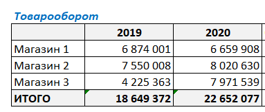
Как видите, товарооборот в 2020 году изменился по отношению к 2019 г. во всех магазинах. У кого-то уменьшился, у кого-то увеличился. И нужно понять, насколько изменение товарооборота конкретного магазина повлияло на общий результат деятельности компании.
Для этого добавим в таблицу следующие столбцы:
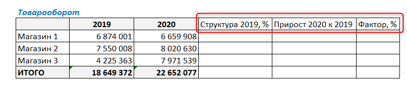
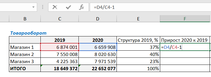
Для начала нашего факторного анализа посчитаем структуру товарооборота в 2019 году. Структура будет показывать долю каждого магазина в суммарных продажах за 2019 год.
Для этого в ячейку Е4 введем следующую формулу:
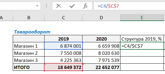
Нужно поделить продажи Магазина 1 на общую сумму продаж. Не забудьте закрепить значение итоговой ячейки C7 в формуле знаками $ ($C$7). Закрепить значение ячейки можно, установив курсор на C7 и нажав клавишу F4 (подробнее об абсолютных и относительных ссылках в *статье*). Это нужно для того, чтобы ссылка на итоговую ячейку не съехала при протягивании формулы вниз.
Для полученного результата выберем процентный формат ячейки и протянем формулу вниз:
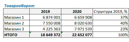
На данном этапе факторного анализа видим, что наибольший вклад в товарооборот компании за 2019 г. внес Магазин 2 — 40%. В итоговой ячейке нужно просуммировать получившиеся проценты, сумма обязательно должна быть равна 100% — это значит, что все посчитано верно.
Далее в ячейке F4 посчитаем прирост продаж 2020 года к 2019. Для этого разделим сумму продаж за 2020 г на сумму за 2019 и отнимем единицу (стандартная формула для расчета изменения показателя).
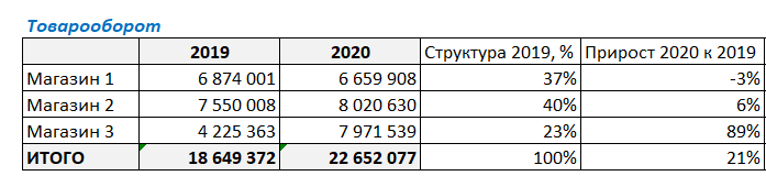
Протянем формулу вниз, захватывая итоговую строку, и увидим, что продажи в 2020 г. в целом по компании выросли на 21% по отношению к предыдущему году. Также видим изменение товарооборота в каждом из магазинов.
И в завершении данного этапа факторного анализа нужно умножить долю магазина на прирост продаж. Для этого в ячейке G4 напишем следующую формулу:
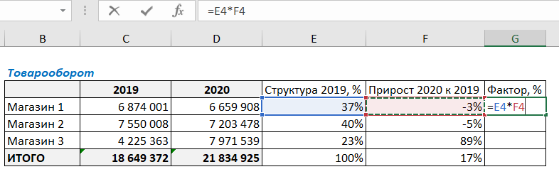
Протянем формулу вниз до итоговой ячейки.
Что же можно увидеть из итоговых результатов факторного анализа по товарообороту?
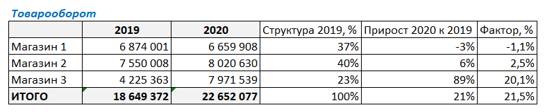
В целом товарооборот, вырос на 21,5% (выведем десятые доли для наглядности). И эти 21,5% складываются из следующих составляющих (факторов):
Фактор “Магазин 1” дал -1,1 % прироста в изменении товарооборота компании (т.е. падение товарооборота, т.к. прирост отрицательный)
Фактор “Магазин 2” для 2,5 % прироста из 21%.
А вот Фактор “Магазин 3” дал 20,1% прироста в составе группы магазинов, и аж 89% по отношению к собственным продажам в предыдущем году.
В итоге:
-1,1% + 2,5% + 20,1% = 21,5%
Таким образом, этот простой пример факторного анализа показывает, что максимальный вклад в прирост товарооборота сделал фактор “Магазин 3”.
Но не будем останавливаться на достигнутом, т.к. нам, во-первых, нужно понять, так ли на самом деле успешен Магазин 3 (ведь конечной целью бизнеса является получение прибыли, а не выручки), а во-вторых, понять, чем можно объяснить такой большой прирост продаж по данному магазину и падение продаж по Магазину 1.
Факторный анализ по операционной прибыли
Что такое операционная прибыль, можно прочитать в статье Что такое прибыль. Виды прибыли
Факторный анализ по операционной прибыли проведем по тем же этапам, что и анализ по продажам. Используем те же дополнительные столбцы и такие же формулы (их можно даже скопировать).
В итоге видим, что Магазин 3, который показывал головокружительный рост выручки, по операционной прибыли уже не такой успешный.
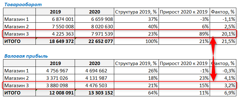
О чем это может говорить? О том, что нужно проводить дополнительный анализ факторов, которые могли повлиять на операционную прибыль. В данном случае в Магазине 3 сильно увеличились издержки (намного сильнее, чем выросла выручка), и при дополнительном анализе нужно понять, какие именно это издержки. Возможно, значительно увеличился штат сотрудников или арендуемая площадь, и т.д.
Магазин 2 показал рост прибыли больше, чем рост выручки. Это может говорить о том, что данный магазин снизил издержки (например, сократился штат сотрудников).
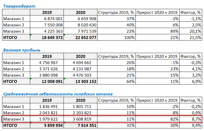
Факторный анализ пример расчета по себестоимости складских запасов
Дополнительно можно провести факторный анализ складских запасов. Это нужно, чтобы понять, за счет чего изменяется выручка.
Проделаем те же шаги, что и на предыдущих двух этапах.
Видим, что у Магазин 3, который показал высокий рост выручки и совсем небольшой рост операционной прибыли, очень сильно выросла сумма складских запасов.
Какой можно сделать предварительный вывод? Например, что Магазин 3, увидев тенденцию к росту продаж, арендовал дополнительную площадь для хранения товарных запасов. А рост выручки хоть и был достаточно высок — но меньше ожидаемого, и в итоге аренда дополнительных площадей для хранения сказалась на прибыли не лучшим образом.
Таким вот нехитрым образом можно провести простой факторный анализ. Конечно, для полноценной аналитики этого может быть недостаточно, нужно учитывать еще множество факторов и составляющих. Но для того, чтобы увидеть общие тенденции, такого простого анализа бывает достаточно.
Более подробно о факторном анализе с примерами расчета можно прочитать в статьях:
Вам может быть интересно: