Excel exist in table

Value exists in a range

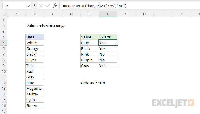
Summary

To test if a value exists in a range of cells, you can use a simple formula based on the COUNTIF function and the IF function. In the example shown, the formula in F5, copied down, is:

where data is the named range B5:B16. As the formula is copied down it returns «Yes» if the value in column E exists in B5:B16 and «No» if not.

Generic formula

Explanation

In this example, the goal is to use a formula to check if a specific value exists in a range. The easiest way to do this is to use the COUNTIF function to count occurences of a value in a range, then use the count to create a final result.

COUNTIF function

The COUNTIF function counts cells that meet supplied criteria. The generic syntax looks like this:

Range is the range of cells to test, and criteria is a condition that should be tested. COUNTIF returns the number of cells in range that meet the condition defined by criteria. If no cells meet criteria, COUNTIF returns zero. In the example shown, we can use COUNTIF to count the values we are looking for like this

Once the named range data (B5:B16) and cell E5 have been evaluated, we have:

COUNTIF returns 1 because «Blue» occurs in the range B5:B16 once. Next, we use the greater than operator (>) to run a simple test to force a TRUE or FALSE result:

By itself, the formula above will return TRUE or FALSE. The last part of the problem is to return a «Yes» or «No» result. To handle this, we nest the formula above into the IF function like this:

This is the formula shown in the worksheet above. As the formula is copied down, COUNTIF returns a count of the value in column E. If the count is greater than zero, the IF function returns «Yes». If the count is zero, IF returns «No».

Slightly abbreviated

It is possible to shorten this formula slightly and get the same result like this:

Here, we have remove the «>0» test. Instead, we simply return the count to IF as the logical_test. This works because Excel will treat any non-zero number as TRUE when the number is evaluated as a Boolean.

Testing for a partial match

To test a range to see if it contains a substring (a partial match), you can add a wildcard to the formula. For example, if you have a value to look for in cell C1, and you want to check the range A1:A100 for partial matches, you can configure COUNTIF to look for the value in C1 anywhere in a cell by concatenating asterisks on both sides:

The asterisk (*) is a wildcard for one or more characters. By concatenating asterisks before and after the value in C1, the formula will count the text in C1 anywhere it appears in each cell of the range. To return «Yes» or «No», nest the formula inside the IF function as above.

An alternative formula using MATCH

As an alternative, you can use a formula that uses the MATCH function with the ISNUMBER function instead of COUNTIF:

The MATCH function returns the position of a match (as a number) if found, and #N/A if not found. By wrapping MATCH inside ISNUMBER, the final result will be TRUE when MATCH finds a match and FALSE when MATCH returns #N/A.

Источник

Test if Value Exists in a Range in Excel & Google Sheets

Download the example workbook

This tutorial demonstrates how to use the COUNTIF function to determine if a value exists in a range.

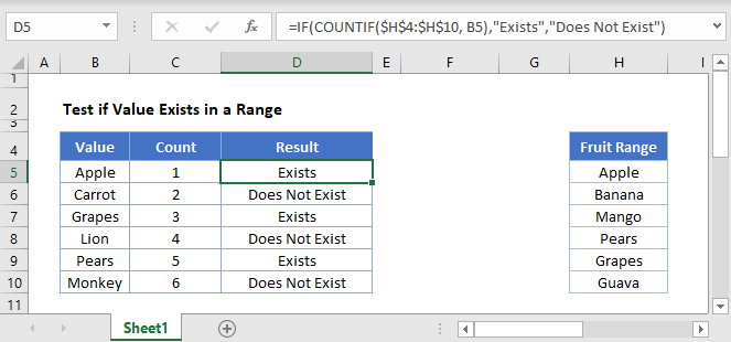
COUNTIF Value Exists in a Range

To test if a value exists in a range, we can use the COUNTIF Function:

The COUNTIF function counts the number of times a condition is met. We can use the COUNTIF function to count the number of times a value appears in a range. If COUNTIF returns greater than 0, that means that value exists.

By attaching “>0” to the end of the COUNTIF Function, we test if the function returns >0. If so, the formula returns TRUE (the value exists).

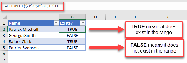
You can see above that the formula results in a TRUE statement for the name “Patrick Mitchell. On the other hand, the name “Georgia Smith” and “Patrick Svensen” does not exist in the range $B$2:$B$31.

You can wrap this formula around an IF Function to output a specific result. For example, if we want to add a “Does not exist” text for names that are not in the list, we can use the following formula:

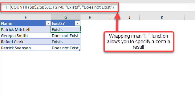
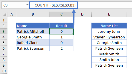
COUNTIF Value Exists in a Range Google Sheets

We use the same formula structure in Google Sheets:

Источник

VBA Check If table Exists in Excel

VBA Check if table Exists in Excel. Let us check if a table exists on the worksheet. And also check if multiple tables are exist on the Sheet. We use ListObjects collection. In this tutorial we have explained multiple examples with explanation. We also shown example output screenshots. You can change table and sheet name as per your requirement. We also specified step by step instructions how to run VBA macro code at the end of the session.

Example to to Check If a table Exists on the Worksheet

Let us see the example to check if a table Exists on the Worksheet using VBA. The sheet name defined as ‘Table‘. And we use table name as ‘MyTable1‘. You can change these two as per your requirement.
Where ListObjects represents the collection.

Output: Here is the following output screenshot of above example macro VBA code.

Check Multiple Tables are exists on the Worksheet

Here is the another example to check if multiple tables are exists on the Worksheet using VBA.

Output: Let us see the following output screenshot of above example macro VBA code. The difference between before and after macro, see the above output screenshot.

Instructions to Run VBA Macro Code or Procedure:

You can refer the following link for the step by step instructions.

Other Useful Resources:

Click on the following links of the useful resources. These helps to learn and gain more knowledge.

Источник

Checking if a value exists anywhere in range in Excel

I want to check if the value of the cell A1 exist anywhere from sheet2!$A$2:$z$50.

IF the value exist then return the value of the 1st Row at the column where the match was found.

but this functions are limited to check if match at a single row / column.

I was hoping for something like =IF(A1,sheet2!$A$2:$Z$50,x1,FALSE) where x = the column where the match was found.

Is there something like that?

4 Answers 4

An array formula like this would work

Press Shift Ctrl Enter together

Say Sheet2 is like:

We want a formula on Sheet1 that will return the value in the header row if that column contains a value to be found. So if A1 contains Good Guy then the formula should return Victor Laszlo

Put the following UDF in a standard module:

User Defined Functions (UDFs) are very easy to install and use:

1. ALT-F11 brings up the VBE window
2. ALT-I ALT-M opens a fresh module
3. paste the stuff in and close the VBE window

If you save the workbook, the UDF will be saved with it. If you are using a version of Excel later then 2003, you must save the file as .xlsm rather than .xlsx

To remove the UDF:

1. bring up the VBE window as above
2. clear the code out
3. close the VBE window

To use the UDF from Excel:

=GetHeader(A1,Sheet2!A1:Z50)

To learn more about macros in general, see:

and for specifics on UDFs, see:

Macros must be enabled for this to work!

We give the UDF the entire range including the header row (although the header row is excluded from the search)

Источник

Check IF a Value Exists in a Range

In Excel, to check if a value exists in a range or not, you can use the COUNTIF function, with the IF function. With COUNTIF you can check for the value and with IF, you can return a result value to show to the user. i.e., Yes or No, Found or Not Found.

Check for a Value in a Range

In the following example, you have a list of names where you only have first names, and now, you need to check if “Arlene” is there or not.

You can use the following steps:

1. First, you need to enter the IF function in cell B1.
   
2. After that, in the first argument (logical test), you need to enter the COUNTIF function there.
   
3. Now, in the COUNTIF function, refer to the range A1:A10.
   
4. Next, in the criteria argument, enter “Glen” and close the parentheses for the COUNTIF Function.
   
5. Additionally, use a greater than sign and enter a zero.
   
6. From here, enter a comma to go to the next argument in the IF, and enter “Yes” in the second argument.
   
7. In the end, enter a comma and enter “No” in the third argument and type the closing parentheses.
   

The moment you hit enter it returns “Yes”, as you have the value in the range that you have searched for.

How this Formula Works

This formula has two parts.

In the first part, we have COUNTIF, which counts the occurrence of the value in the range. And in the second part, you have the IF function that takes the values from the COUNTIF function.

So, if COUNTIF returns any value greater than which means the value is there in the range IF returns Yes. And if COUNTIF returns 0, which means the value is not there in the range and it returns No.

Check for a Value in a Range Partially

There counts to be a situation where you want to check for partial value from a range. In that case, you need to use wildcard characters (asterisk *).

In the following example, we have the same list of names but here is the full name. But we still need to look for the name “Glen”.

The value you want to search for needs to be enclosed with an asterisk, which we have used in the above example. This tells Excel, to check for the value “Glen” regardless of what is there before and after the value.

Источник