Excel every second row

In this post I will show you how to select every other row in Excel. Like many tasks in Excel, there is more than one way to achieve this. Here I show you 5 ways to select every other row in Excel. These 5 tips will improve your data manipulation skills.

Use the contents table below to skip to each section.

1. Using CTRL and mouse click
2. Conditional Formatting
3. Format Data as a Table
4. ‘Go To Special’ hack
5. VBA (automation)

Using CTRL and Mouse Click To Select Every Other Row

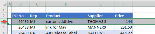
The simplest way to select every other row in Excel is to hold down down the CTRL button on your keyboard (⌘ on MAC) and then the number of the rows you want to select.

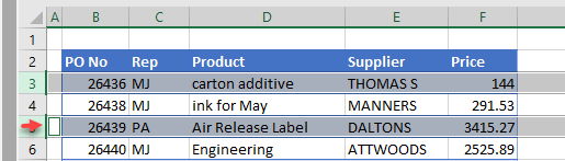
Clicking on the row number itself highlights the whole row. By holding down CTRL, we are able to select every other row or even a bunch of single cells. This sort of selection is referred to as a non-contiguous range.

To deselect a row, simply click on it again. You can also perform a non-contiguous selection on individual cells and columns.

The advantage of this technique is it’s speed. You can very quickly select the rows you want to alter and then apply the change to all of them in one go.

The downside to this technique is when you have large datasets and it becomes too laborious to select all the rows you want manually.

You can also see from our example that the row selection exceeds the boundaries of our data which is also something you may not want to do.

Highlight Every Other Row With Conditional Formatting

Conditional formatting alters the look of a cell based upon the value within it. It is a very flexible tool and we can use it to highlight every other row in a data set. We can use it to highlight (select) every other row in Excel.

In this example, I want to color alternate rows, starting with the first row after the header.

First I select the data I want to apply the Conditional Formatting to (excluding the header), then hit:

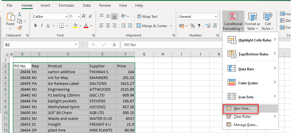
Home –> Conditional Formatting –> New Rule…

Doing this will bring up the New Formatting Rule dialog box. From the options available, click on ‘Use a formula to determine which cells to format’.

This will change the dialog box to allow you to enter a formula that your conditional formatting will abide by. In the box, insert the following formula:

=MOD(ROW(B2),2)=0

NOTE: Substitute B2 above for the top-left most cell in your selection.

Formula Explainer

The MOD function returns the remainder of a division expression. So if you passed in the number 3 to be divided by 2, you’d get 1.

The ROW function returns the number of the row of the cell reference that you pass in. So in this case, cell B2 is row number 2.

So by passing in the row number, and dividing it by 2 using the MOD function, we’ll be able to tell if a row number is odd or even. Odd row numbers will return 1, even row numbers will return 0.

When the formula evaluates to 0, our conditional formatting rule is applied!

Next you can set the color of that you’d like the alternate rows to be. To do this, simply click ‘Format…’ –> Fill and select your chosen color. Then hit OK.

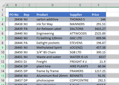
Click OK again to exit out of the Conditional Formatting rules dialog box and your rule will be applied immediately to your selection.

Format Data As A Table

Excel has a built-in feature to format ranges as tables. There are many advantages to using tables in Excel and you can learn more about using them from this great post by Easy Excel on Data Tables In Excel.

One of those benefits is that the data is formatted nicely with alternate colored rows, making it simpler for us to eye over the data.

To convert a range to a data table, first select the data, including a header if you have one, and then click:

Keyboard Shortcut

To quickly insert a table, select your data, then press CTRL + T on the keyboard.

The ‘Create Table’ dialog box will appear. Double-check that the range of cells you are going to format as a table is correct.

If you need to make an adjustment, you can overwrite the cell range in the box or simply click the small upward arrow, and then select the cells from your worksheet using the mouse.

If you data has headers, make sure the ‘My table has headers’ box is checked. Click OK.

Your data will now be formatted as a table object. The default color formatting will be applied and every other row will be colored.

You can quickly adjust the color formatting by selecting any cell within your data table and then clicking Table Design up on the ribbon.

In the ‘Table Styles’ section, you have the option to change the table’s color from a selection of pre-set formats. Customization is also available.

‘Go To Special’ Hack

This technique works great if you want to select every other row in Excel within your data set to then delete it.

First we create a “helper” column in the first column to the left of our data set. Give it a header to clearly mark it’s purpose, it will be deleted later on.

In the first row of the helper column, insert an ‘X’. Then click on this cell and drag your mouse down to the cell below, so that both of the cells are now selected.

Now the first to cells are selected, notice the small green square in the bottom-right of the selected cells – this is the Auto Fill Handle.

Click and hold the Auto Fill Handle, and drag the mouse down to extend the selection to all of the rows in your data set.

Auto Fill Handle

The cursor changes to a small black plus sign when you mouse over the auto fill handle to indicate it is active.

Clicking and dragging down will extend the “X then blank” pattern to all of the cells you select.

Alternatively, you can double-click the fill handle and it will automatically extend down to the end of your data set.

The auto fill handle is a really useful feature on Excel. You can read more about it’s functionality in this post on 6 Ways To Use The Fill Handle In Excel

Now we have created a recognizable pattern of “X then blank” for every 2 cells in the helper column. With these cells still selected, click:

Home –> Find & Select –> Go To Special…

This will open the ‘Go To Special’ dialog box. Select the ‘Blanks’ radio button then click OK.

Excel will now create a non-contiguous cell selection on the blank cells in the helper column. Now we can right-click on any of the selected cells and click Delete. This will launch the ‘Delete’ dialog box where you can then select Entire Row and then click OK.

Every other row will be deleted and the data will be pushed up into the gaps.

You can now delete your helper column

VBA (Automation)

VBA (visual basic for applications) is Excel’s built-in programming language. We can use this small script to automatically select every other row of a given range.

To use the script, copy and paste it into a new module in the VBA Editor.

To open a new module, go to Developer –> Visual Basic. If you don’t see the Developer tab on the ribbon, you’ll need to activate it first.

When in the VBA Editor, click Insert –> Module

To run this code, a user will need to make a selection of cells that they want to select every other row from first. The code works by looping through the selected range and adds every other row to a range variable which is then selected at the end of the programme.

Summary

Here we have looked at 5 different ways to select every other row in Excel. As we have seen, there are many methods available for us to do this from conditional formatting to automated selection via VBA.

See all How-To Articles

This tutorial demonstrates how to select every other row in Excel and Google Sheets.

When you’re working with data in Excel, you have a need to select the data in every other row. There are a few ways to select every other row.

Select Every Other Row

Keyboard and Mouse

1. Click on the row header to select the first row.

1. Holding down the CTRL key on the keyboard, click in the row header of the second row.

1. With the CTRL key still held down, click on every other row header until all the rows you need are selected.

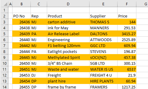
Cell Format and Filter

You can use Format as Table and filtering to select every other row.

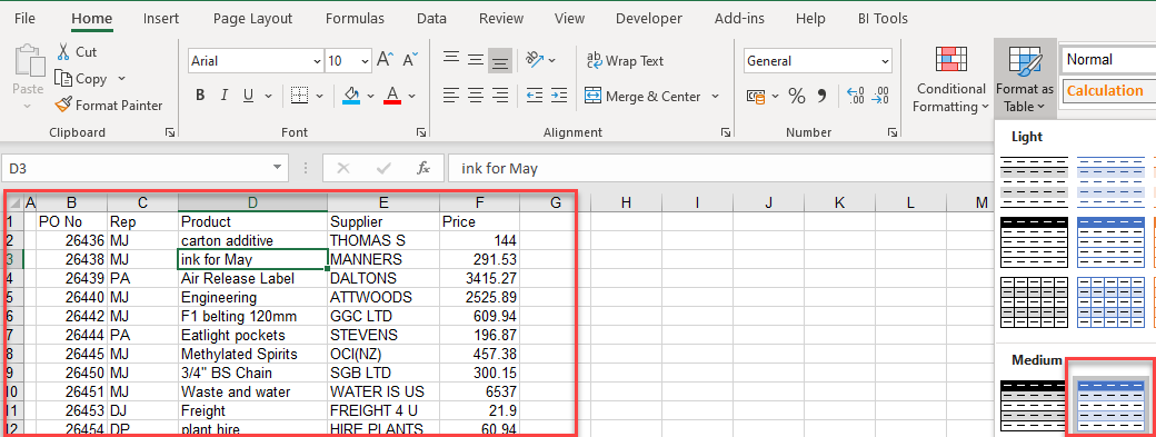
1. Highlight the cells whose rows you wish to select. In the Ribbon, go to Home > Cells > Format as Table and select the formatting.

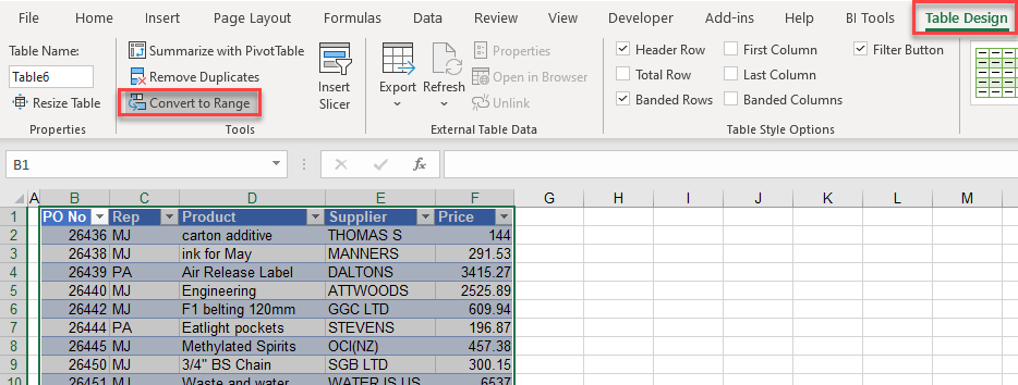
1. Then, to remove the table, in the Ribbon, select Table > Convert to Range.

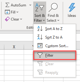
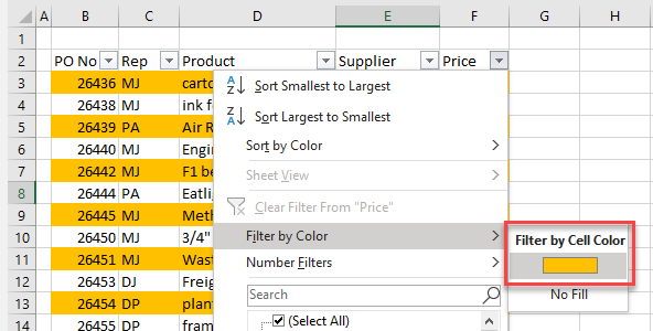
1. Next, in the Ribbon, select Home > Editing > Sort & Filter > Filter.

1. Click the drop-down arrow on any of the column headings and select Filter by Color.

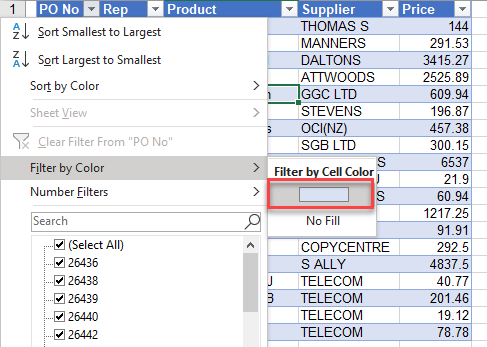
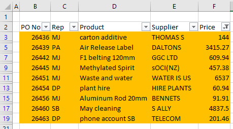
1. Every second row is now filtered for. Select these rows.

Conditional Formatting and Filter

You can use Conditional Formatting and Filtering to select every other row.

1. Highlight the cells whose rows you wish to select. In the Ribbon, go to Home > Cells >Conditional Formatting.

1. Select (1) Use a formula to determine which cells to format and then (2) enter the formula:

=MOD(ROW(B3),2)=0

Then (3) click on Format…

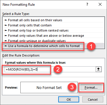
• The ROW Function returns the row number of the cell.
• The MOD Function, here, tests whether a number is even or odd by returning the remainder of the ROW formula divided by 2.

1. In the Fill tab, select the color to format each alternate row, and click OK.

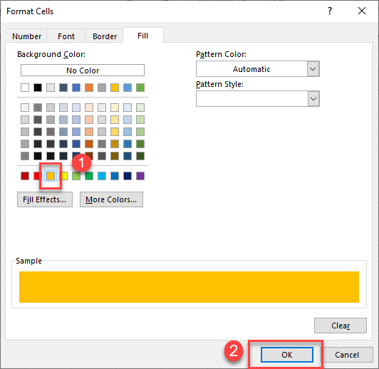
1. Click OK again to apply the formatting to your worksheet.

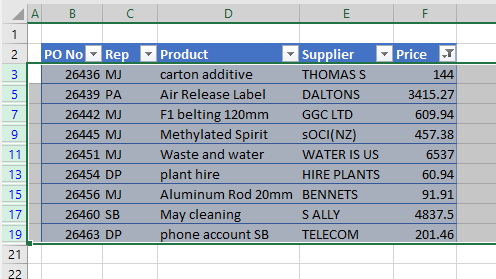
1. As with Format as a Table, you can now Filter by Color to select every alternate row.

All the rows with the yellow cells are shown.

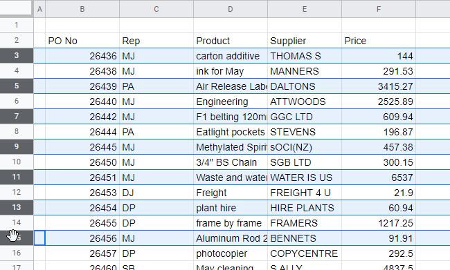
Select Every Other Row in Google Sheets

As with Excel, you can select every other row in a Google Sheet by selecting the first row and then holding down the CTRL key and selecting each alternate row thereafter.

You can also use conditional formatting and filtering to select every other row.

1. Highlight the cells whose rows you wish to select. In the Menu, select Format > Conditional Formatting.

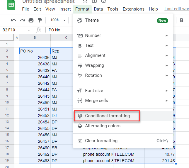
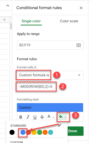
1. Select (1) Custom formula is from the Format cells if… list and then (2) type in the following formula:

=MOD(ROW(B3),2)=0

Then (3) select the color you wish every other row in the selection to be formatted with.

1. Click Done to format the sheet.
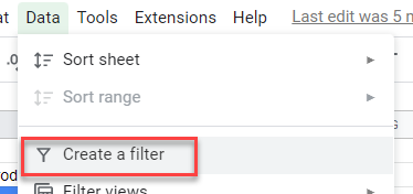
2. Then create a filter to filter the rows by color.
   In the Menu, select Data > Create a filter.

1. In the filter drop-down list at the top of one of the columns, select Filter by Color > Fill Color and then select which color to filter on.

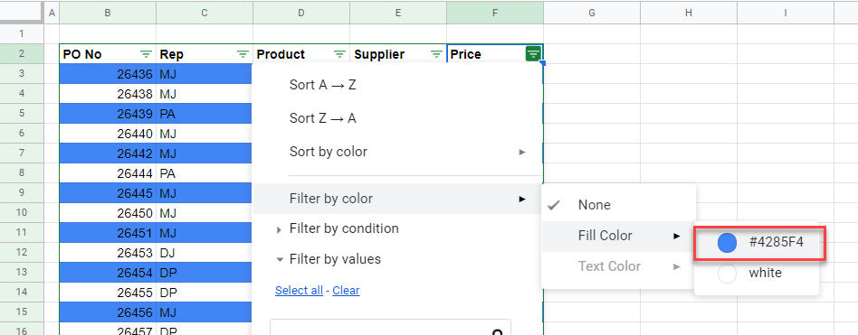
Every other row is now shown.

See also: How to Display Data With Banded Rows

Когда мы используем рабочий лист, иногда нам нужно выбрать каждую вторую или n-ю строку листа для форматирования, удаления или копирования. Вы можете выбрать их вручную, но если есть сотни строк, этот метод не лучший выбор. Вот несколько уловок, которые могут вам помочь.

Выберите каждую вторую или n-ю строку с помощью VBA

Выберите каждую вторую или n-ю строку с помощью Kutools for Excel

---

Выберите каждую вторую или n-ю строку с помощью VBA

В этом примере я выберу одну строку с двумя интервалами. С кодом VBA я могу закончить это следующим образом:

1. Выделите диапазон, который вы хотите выделить, каждую вторую или n-ю строку.

2.Click Застройщик > Визуальный Бейсик, Новый Microsoft Visual Basic для приложений появится окно, щелкните Вставить > Модули, и введите в модуль следующий код:

Sub EveryOtherRow()
Dim rng As Range
Dim InputRng As Range
Dim OutRng As Range
Dim xInterval As Integer
xTitleId = "KutoolsforExcel"
Set InputRng = Application.Selection
Set InputRng = Application.InputBox("Range :", xTitleId, InputRng.Address, Type:=8)
xInterval = Application.InputBox("Enter row interval", xTitleId, Type:=1)
For i = 1 To InputRng.Rows.Count Step xInterval + 1
    Set rng = InputRng.Cells(i, 1)
    If OutRng Is Nothing Then
        Set OutRng = rng
    Else
        Set OutRng = Application.Union(OutRng, rng)
    End If
Next
OutRng.EntireRow.Select
End Sub

3. затем нажмите кнопку для запуска кода. Появится диалоговое окно для выбора диапазона. Смотрите скриншот:

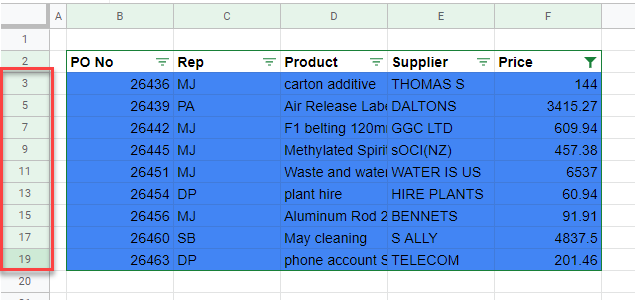
4. Нажмите OK, и в этом случае я ввожу 3 в другом всплывающем диалоговом окне в качестве строки интервала. Смотрите скриншот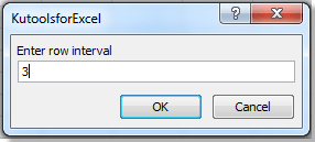

5. Нажмите OK, и выбрана каждая третья строка. Смотрите скриншот:

Вы можете изменить интервал по мере необходимости во втором KutoolsforExcel Диалог.

---

Выберите каждую вторую или n-ю строку с помощью Kutools for Excel

С кодом VBA вы можете выбрать только одну строку с указанными интервалами, если вам нужно выбрать две, три или другие строки с указанными интервалами, Kutools for Excel поможет вам решить эту проблему легко и удобно.

После бесплатная установка Kutools for Excel, пожалуйста, сделайте следующее:

1. Нажмите Кутулс > Select > Select Interval Rows & Columns…, См. Снимок экрана:

2. в  Select Interval Rows & Columns диалоговое окно, щелкните кнопку для выбора нужного вам диапазона, выберите Rows or Columns от Select разделе., и укажите желаемое число в Interval of поле ввода и Rows поле ввода. Смотрите скриншот:

Ноты:
1. Если вам нужно выбрать все остальные строки в выделенном фрагменте, введите 2 в поле Интервалы ввода и 1 в поле Rows поле ввода.

2. Если вы хотите выделить всю нужную строку, вы можете установить флажок Select entire rows опцию.

---

Заштрихуйте каждую вторую строку или n-ю строку с помощью Kutools for Excel

Если вы хотите заштриховать диапазоны в каждой второй строке, чтобы данные выглядели более выдающимися, как показано на скриншоте ниже, вы можете применить Kutools for ExcelАвтора Alternate Row/Column Shading функция для быстрого выполнения работы.

После бесплатная установка Kutools for Excel, пожалуйста, сделайте следующее:

1. Выберите диапазон ячеек, для которых требуется интервал затенения, щелкните Кутулс > Format > Alternate Row/Column Shading.

2. в Alternate Row/Column Shading диалог, выполните следующие действия:

1) Выберите строки или столбцы, которые хотите заштриховать;

2) Выберите Conditional formatting or стандартное форматирование как вам нужно;

3) Укажите интервал штриховки;

4) Выберите цвет штриховки.

3. Нажмите Ok. Теперь диапазон закрашен в каждой n-й строке.

Если вы хотите убрать затенение, отметьте Удалить существующее затенение альтернативной строки вариант в Альтернативное затенение строки / столбца Диалог.

---

Статьи по теме:

• Выберите каждый n-й столбец в Excel
• Копировать каждую вторую строку
• Удалить каждую вторую строку
• Скрыть каждую вторую строку

Была ли эта статья полезной?

Watch Video – How to Highlight Alternate (Every Other Row) in Excel

Below is the complete written tutorial, in case you prefer reading over watching a video.

Conditional Formatting in Excel can be a great ally in while working with spreadsheets.

A trick as simple as the one to highlight every other row in Excel could immensely increase the readability of your data set.

And it is as EASY as PIE.

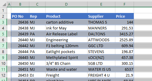
Suppose you have a dataset as shown below:

Let’s say you want to highlight every second month (i.e., February, April and so on) in this data set.

This can easily be achieved using conditional formatting.

Highlight Every Other Row in Excel

Here are the steps to highlight every alternate row in Excel:

1. Select the data set (B4:D15 in this case).
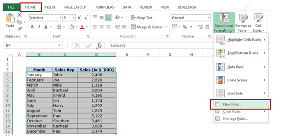
2. Open the Conditional Formatting dialogue box (Home–> Conditional Formatting–> New Rule) [Keyboard Shortcut – Alt + O + D].
3. In the dialogue box, click on “Use a Formula to determine which cells to format” option.
4. In Edit the Rule Description section, enter the following formula in the field:
   =MOD(ROW(),2)=1

1. Click on the Format button to set the formatting.
2. Click OK.

That’s it!! You have the alternate rows highlighted.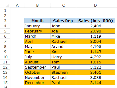

How does it Work?

Now let’s take a step back and understand how this thing works.

The entire magic is in the formula =MOD(ROW(),2)=1. [MOD formula returns the remainder when the ROW number is divided by 2].

This evaluates each cell and checks if it meets the criteria. So it first checks B4. Since the ROW function in B4 would return 4, =MOD(4,2) returns 0, which does not meet our specified criteria.

So it moves on to the other cell in next row.

Here Row number of cell B5 is 5 and =MOD(5,1) returns 1, which meets the condition. Hence, it highlights this entire row (since all the cells in this row have the same row number).

You can change the formula according to your requirements. Here are a few examples:

• Highlight every 2nd row starting from the first row =MOD(ROW(),2)=0
• Highlight every 3rd Row =MOD(ROW(),3)=1
• Highlight every 2nd column =MOD(COLUMN(),2)=0

These banded rows are also called zebra lines and are quite helpful in increasing the readability of the data set.

If you plan to print this, make sure you use a light shade to highlight the rows so that it is readable.

Bonus Tip: Another quick way to highlight alternate rows in Excel is to convert the data range into an Excel Table. As a part of the Excl Table formatting, you can easily highlight alternate rows in Excel (all you need is to use the check the Banded Rows option as shown below):

You May Also Like the Following Excel Tutorials:

• Creating a Heat Map in Excel.
• How to Apply Conditional Formatting in a Pivot Table in Excel.
• Conditional Formatting to Create 100% Stacked Bar Chart in Excel.
• How to Insert Multiple Rows in Excel.
• How to Count Colored Cells in Excel.
• How to Highlight Blank Cells in Excel.
• 7 Quick & Easy Ways to Number Rows in Excel.
• How to Compare Two Columns in Excel.
• Insert a Blank Row after Every Row in Excel (or Every Nth Row)
• Apply Conditional Formatting Based on Another Column in Excel
• Select Every Other Row in Excel