We can evaluate a basic excel formulaThe term «basic excel formula» refers to the general functions used in Microsoft Excel to do simple calculations such as addition, average, and comparison. SUM, COUNT, COUNTA, COUNTBLANK, AVERAGE, MIN Excel, MAX Excel, LEN Excel, TRIM Excel, IF Excel are the top ten excel formulas and functions.read more by using two methods –
- Using F9 Key
- Using the “Evaluate” Tool
Table of contents
- How to Evaluate Formula in Excel?
- #1 Evaluate Excel Formula Using F9 Key
- Example 1
- Example #2
- #2 Evaluate Formula by Using EVALUATE FORMULA Option
- Things to Remember
- Recommended Articles
- #1 Evaluate Excel Formula Using F9 Key
Now let us discuss each of the methods in detail and an example.
You can download this Evaluate Formula Excel Template here – Evaluate Formula Excel Template
#1 Evaluate Excel Formula Using F9 Key
To understand big formulas, we need first to understand parts of the formula step by step, and this is called an evaluation of the formula or debugging.
Example 1
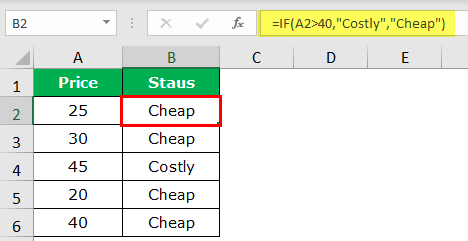
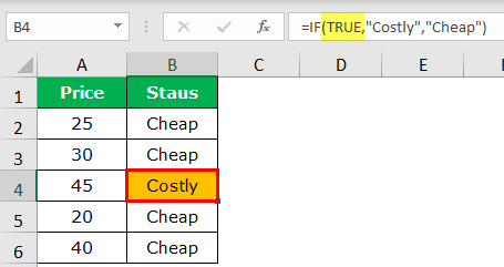
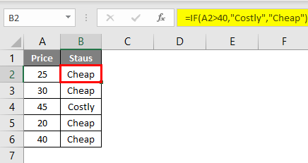
For example, look at the below formula for this example.
If you do not understand anything from the formula, we can evaluate it by pressing the F9 key.
The F9 key is used to quickly evaluate and debug the formula to understand and efficiently work with Excel. Using this F9 key, we can determine only the part of the formula by replacing the actual formula with the result of the formula.
IIn the above example, we have applied a logical test, i.e., A2>40. Based on the logical test, we are analyzing the price status. If the price is >40, then we need the result as “Costly,” or else we need the result as “Cheap.” So, IF conditionIF function in Excel evaluates whether a given condition is met and returns a value depending on whether the result is “true” or “false”. It is a conditional function of Excel, which returns the result based on the fulfillment or non-fulfillment of the given criteria.
read more tests the logical test and returns “Costly” if the logical test is “TRUE” or if the logical test is “FALSE,” it will return “Cheap.”
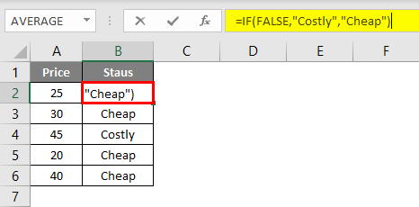
In the B2 cell, we have got the result as “Cheap” to understand how we got this result. Let us evaluate the logical part of the formula.
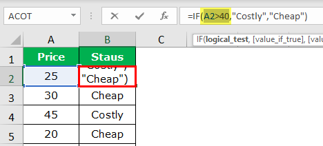
In the formula, the bar selects only the logical test part of the formula.
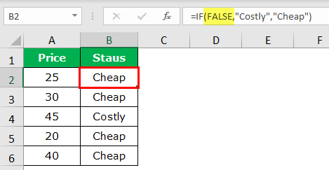
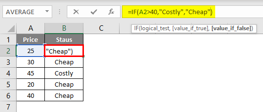
Once the logical test part is selected, press the F9 key, and see what the result is.
It says “FALSE” because the A2 cell price value is not >40, so the logical test is “FALSE.” Since the logical test is FALSE, we got the result as “Cheap.”
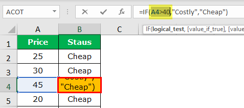
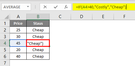
Now, we need to go to cell B4, where we have the result of “Cheap.” Select the logical test part and press the F9 key in that cell.
Now, press the F9 key to see the result of the logical test.
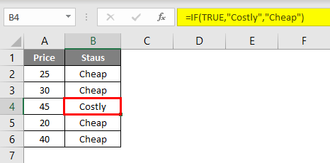
The logical test result is “TRUE.” Since we have applied the result as “Costly” for the TRUE part, we got the same result in the B4 cell because the price of the A4 cell is >40.
But when it comes to cell B6, we got the result as “Cheap” even though the price is 40; we have applied the logical test as >40, not >=40.
Example #2
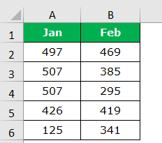
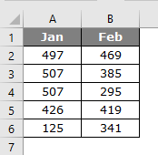
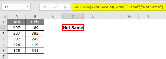
Now, take a look at one more example of evaluating the formula. Let us take a look at the below data.
We need to check whether Jan’s total equals Feb’s total in the above table. If both the totals are equal, we should get the result as “Same” or “Not Equal.”
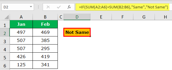
We have applied the formula below:
=IF(SUM(A2:A6)=SUM(B2:B6),”Same”,”Not Same”)
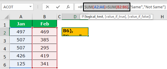
We have applied two SUM functions to get the total Jan and Feb, respectively. Therefore, we must select both the SUM functions in the excelThe SUM function in excel adds the numerical values in a range of cells. Being categorized under the Math and Trigonometry function, it is entered by typing “=SUM” followed by the values to be summed. The values supplied to the function can be numbers, cell references or ranges.read more equation in the formula.
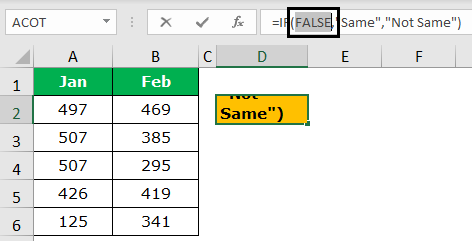
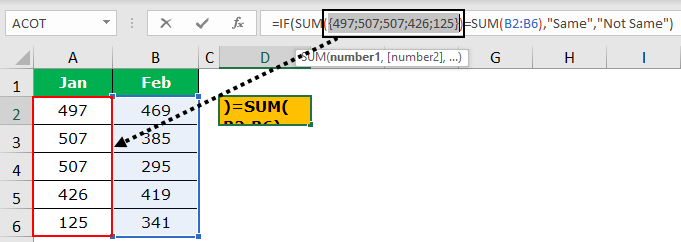
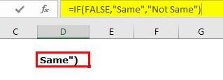
Press the F9 key and let us see what the result is.
We got the result as “FALSE” because Jan’s total equals Feb’s total. So, how do we know Jan’s total is not equal to Feb’s total?
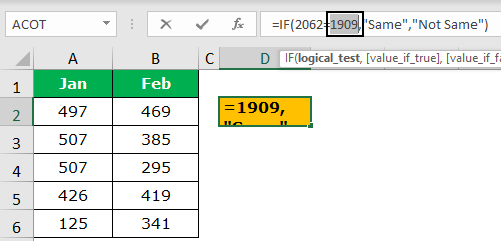
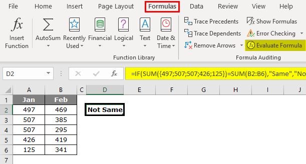
Select only the first SUM function and press the F9 key to check only Jan total.
So, Jan’s total is 2062. Similarly, evaluate Feb’s total.
Feb total is 1909, so the logical test is “FALSE,” and the result is “Not Same.”
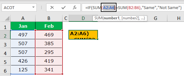
To see the values of the SUM function, consider selecting only the cell range part in the SUM function.
Now press the F9 key; we should see all the cells’ A2 to A6 values.
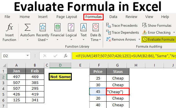
#2 Evaluate Formula by Using EVALUATE FORMULA Option
One more way of evaluating the formula is using the built-in excel featureThe top features of MS excel are — Shortcut keys, Summation of values, Data filtration, Paste special, Insert random numbers, Goal seek analysis tool, Insert serial numbers etc.
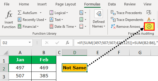
read more “Evaluate Formula” option. This option is available under the “FORMULA” tab.
- Step 1: To use this feature, we must select the formula cell we want to evaluate and click on.
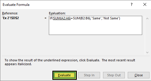
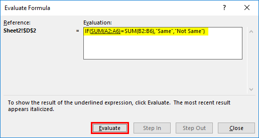
- Step 2: As soon as we click on this button, we get the below window.
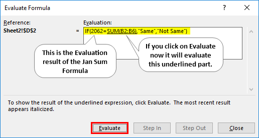
- Step 3: Now click on “Evaluate” it will evaluate the underlined part.
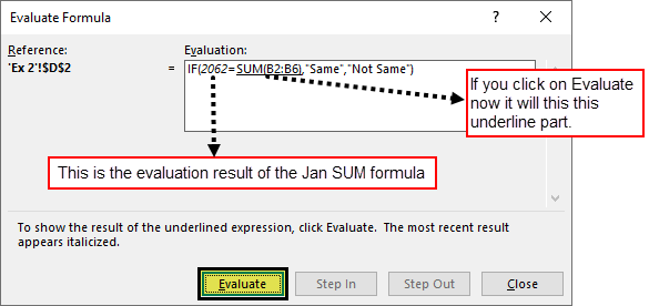
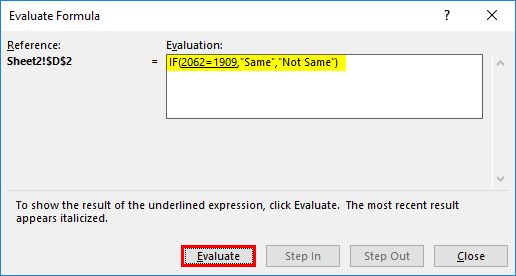
- Step 4: Click on “Evaluate” to evaluate the second SUM function.
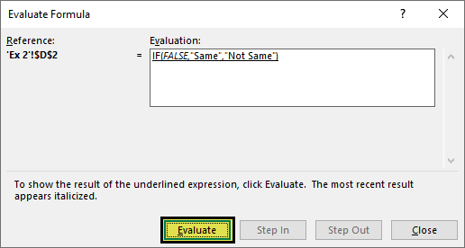
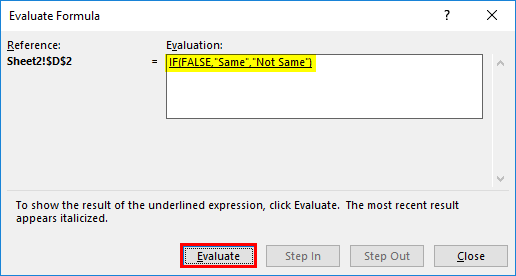
- Step 5: Now, both the equations are selected simultaneously. Click on “Evaluate.” It will show whether the logical test is “TRUE” or “FALSE.”
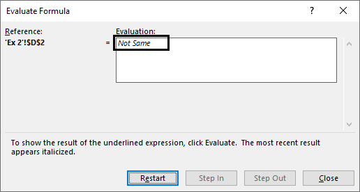
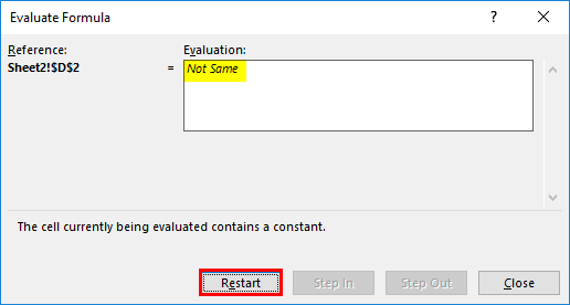
- Step 6: Now, the entire formula is selected, so click on “Evaluate” one last time it will show the final result.
So, the result is “Not Same” because Jan’s total is not equal to Feb’s total.
Things to Remember
We need to be wary of the F9 key because we should consider and press the “Esc” key when evaluating the formula. Otherwise, it will replace calculated results.
For example, we have evaluated all the cell values in the above example.
Now, if we press the “Enter” key, we may get the formula as it is.
So, we need to be careful in this aspect of the F9 key. Furthermore, once its calculated values or cell values replace the formula, it is no longer a dynamic formula. So, we need to be careful in this area while debugging the formula.
Recommended Articles
This article is a guide to the Evaluate Formula in Excel. Here, we discuss evaluating the formula using two methods: 1) F9 Key and 2) Evaluate tool, along with examples and a downloadable Excel template. You may also look at these useful functions in Excel: –
- Insert Formula in Excel
- Create Formula in Excel
- Excel Formula Not Working
- Advanced Excel Formulas
Evaluate Formula in Excel (Table of Contents)
- Evaluate Formula in Excel
- How to Use Evaluate Formula Using F9 Key in Excel?
Evaluate Formula in Excel
When you try to solve complex problems in excel, we might fail most of the time. When we decided to search on the internet, we may get a solution that is readymade, but it is very hard to understand due to the nested formulas they have used.
The good thing is we got the solution that we wanted but not understanding the formula is not a good sign because in the future, if we want to alter or change the references of the formula, we must know how the formula is working.
So, in such situations, it is important to understand the formula, so to understand the formula, we can use the “Evaluate Formula” tool in excel. In this article, we will take you through the process of evaluation of the formula.
How to Use Evaluate Formula Using F9 Key in Excel?
As I told to understand big formulas, we need first to understand parts of the formula step by step, and this is called an evaluation of the formula or debugging.
For an example, look at the below formula for this example.
If you don’t understand anything from the formula, we can evaluate part by part by pressing the F9 key.
The F9 key is used to quickly evaluate and debug the formula to understand and efficiently work with excel. Using this F9 key, we can evaluate only the part of the formula by replacing the actual formula with the result of the formula.
You can download this Evaluate Formula Excel Template here – Evaluate Formula Excel Template
Example #1
In the above example, we have applied a logical test, i.e. A2>40. Based on the logical test, we are analyzing the price status. If the price is >40, then we need the result as “Costly”, or else we need the result as “Cheap”. So, IF condition tests the logical test and returns “Costly” if the logical test is TRUE or if the logical test is FALSE, it will return “Cheap”.
In cell B2, we have got the result as “Cheap”, to understand how we got this result, let’s evaluate the logical part of the formula.
The formula bar selects only the logical test part of the formula.
Once the logical test part is selected, press the F9 key and see what the result is.
It says “FALSE” because in the A2 cell price value is not >40, so the logical test is FALSE. Since the logical test is FALSE, we got the result as “Cheap”.
Now go to cell B4, where we have the result of “Cheap”. In that cell, select the logical test part and press the F9 key.
Now press the F9 key to see the result of the logical test.
The logical test result is TRUE. Since we have applied the result as “Costly” for the TRUE part, we got the same result in the B4 cell because the price of is A4 cell is >40.
But when it comes to cell B6, we got the result as Cheap even though the price is 40; this is because we have applied the logical test as >40, not >=40.
Example #2
Now take a look at one more example of evaluating the formula. Take a look at the below data.
In the below table, we need to check whether the Jan total is equal to the Feb total. If both the totals are equal, we should get the result as “Same” or else “Not Equal”.
I have applied the formula as below.
=IF(SUM(A2:A6)=SUM(B2:B6),”Same”,”Not Same”)
I have applied two SUM function to get the total Jan & Feb respectively. Select both the SUM functions equation in the formula.
Press the F9 key and see what the result is.
We got the result as FALSE because Jan total is equal to Feb total. How do you know Jan total is not equal to Feb total???
To check only Jan total, select only the first SUM function and press the F9 key.
So, Jan total is 2062; similarly, evaluate for Feb total.
Feb total is 1909, so the logical test is FALSE, and the result is “Not Same”.
To see the values of the SUM function, considering selecting only the cell range part in the SUM function.
Now press the F9 key; we should see all the values from the cells A2 to A6.
Evaluate Formula Feature
One more way of evaluating the formula is by using the built-in excel feature “Evaluate Formula” option. This option is available with excel under the FORMULA tab.
To use this feature, select the formula cell that we want to evaluate and click on this feature.
As soon as we click on this button, we get the below window.
Now click on “Evaluate”, it will evaluate the underlined part.
Click on Evaluate to evaluate the second SUM function.
Both the equations are selected simultaneously, and click on Evaluate; it will show whether the logical test is TRUE or FALSE.
Now the entire formula is selected, so click on Evaluate one last time it will show the final result.
So, the result is “Not Same” because Jan total is not equal to Feb total.
Things to Remember
We need to be wary of the F9 key because when we are evaluating the formula, we should just evaluate and press the Esc key; otherwise, it will replace it with calculated results. For example, in the above example, we have evaluated all the cell values.
Now, if I press enter key, we will get the formula as it is.
So, in this aspect of the F9 key, we need to be careful. Once its calculated values or cell values replace the formula, it is no longer a dynamic formula, so this is the one area we need to be careful of while debugging the formula.
Recommended Article
This is a guide to Evaluate Formulas in Excel. Here we discuss How to Use Evaluate Formula Using F9 Key in Excel along with practical examples and a downloadable excel template. You can also go through our other suggested articles –
- Not Equal To Excel
- Excel Logical Test
- Basic Excel Formulas
- LOOKUP Formula in Excel
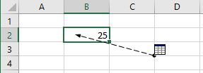
- tracing tools to see the cell dependencies and cell dependents,
- checking error values.
Note: In Excel, formulas are evaluated in the natural order. In other words, if the formula in cell C2 depends on the result of the formula in cell A2, Excel evaluates cell A2 before calculating cell C2.
A simple way to evaluate a part of a formula
You can use a simpler way to evaluate a part of a formula in Excel:
1. Select the cell that contains the formula.
2. Double-click the cell (or activate a cell and press F2) to get into Edit mode (see more about modifying cell data).
3. Select the part of the formula you want to evaluate:
- Using the mouse:
Highlight the part of the formula:
- Using the keyboard:
Press Shift and use the navigation keys.
4. Press F9.
Excel displays the calculated result of the selected part of the formula:

5. You can evaluate other parts of the formula:

or press Esc to cancel and return your formula to its previous state.
Run the Formula Evaluator
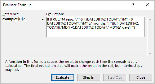
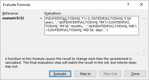
The Evaluate Formula dialog box shows a formula being calculated one step at a time.
To run the Formula Evaluator, select the cell that contains the formula, and on the Formulas tab, in the Formula Auditing group, click Evaluate Formula:

In the Evaluate Formula dialog box:
- Click the Evaluate button repeatedly to see the intermediate results as the formula is calculated. The result of the evaluation is shown in italics:
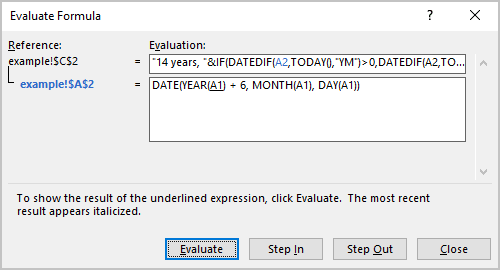
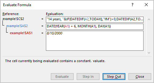
- If the underlined part of the formula is a reference to another formula, click the Step In button to display the other formula in the Evaluation box:
- Click the Step Out button to go back to the previous cell and formula:
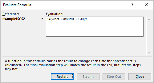
- Click the Restart button to return the evaluation:
Tracing cell relationships
Cell dependencies (in Microsoft Excel, cell precedents)
A formula cell dependencies are all the cells that contribute to the formula result. A direct dependency (in Microsoft Excel, direct precedents) is a cell you use directly in the formula. An indirect dependency (in Microsoft Excel, indirect precedents) is a cell that isn’t used directly in the formula but is used by a cell you refer to.
For example:
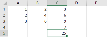
- the cells C1:C3 contain the sum of the columns A and B,
- the cell C4 has a value of 7,
- the cell C5 contains the formula = SUM (C1:C4).
To see the cell dependencies, activate the cell, then on the Formulas tab, in the Formula Auditing group, click the Trace Precedents button:

Excel displays the direct dependencies for the cell C5:
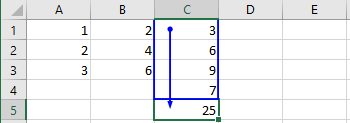
To see the next level of the dependencies, click the Trace Precedents button again:
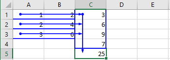
Thus, to see all dependencies, you need to click the Trace Precedents button as many times as many precedent levels are used in the spreadsheet.
Notes:
- If the sheet has a dependency on another sheet or workbook, you will see the arrow like this:
- See also how to select special types of cells.
Cell dependents
Cell dependents include all formula cells that use the cell. The formula cell can be a direct dependent or an indirect dependent.
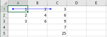
The example is the same as for the dependencies.
To see the cell dependents, activate the cell, then on the Formulas tab, in the Formula Auditing group, click the Trace Dependents button:

Excel displays the direct dependents for the cell A1:
To see the next level of the dependents, click the Trace Dependents button again:
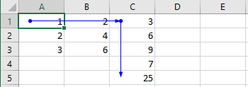
Thus, to see all dependents, you need to click the Trace Dependents button as many times as many dependent levels are used in the spreadsheet.
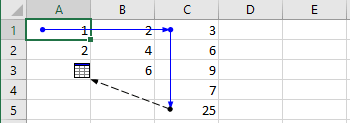
Note: If the sheet has dependents in another sheet or even workbook, you will see the arrow like this:
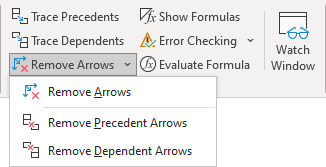
Remove arrows
To remove arrows, on the Formulas tab, in the Formula Auditing group:
- Click the Remove Arrows button to remove all arrows for precedents and dependents,
- Click the Remove Arrows button, then select Remove Precedent Arrows to remove only arrows for precedents,
- Click the Remove Arrows button, then select Remove Dependent Arrows to remove only arrows for dependents:
See how to select special types of cells for more details.
See also this tip in French:
Évaluer la formule dans Excel.
Description
- Select the cell that you want to evaluate.
- On the Formulas tab, in the Formula Auditing group, click Evaluate Formula.
- Click Evaluate to examine the value of the underlined reference.
- Continue until each part of the formula has been evaluated.
- To see the evaluation again, click Restart.
Contents
- 1 How does evaluate formula work?
- 2 How do you evaluate complex Formulas in Excel?
- 3 What is evaluation in Excel?
- 4 What does evaluate mean in Excel?
- 5 What are the advanced Excel formulas?
- 6 How do you evaluate a spreadsheet?
- 7 What will the following expression evaluate to in Spreadsheet 2 3 * 4 5?
- 8 What are the 20 Excel functions?
- 9 What are the 5 functions in Excel?
- 10 What are the top 10 Excel formulas?
- 11 How do you check if Excel formula is correct?
- 12 What is the value of the expression c 6 3 *?
- 13 When writing formulas for Excel All formulas must begin with an?
- 14 What will the following code do a B 18 in python?
- 15 What are Excel formulas?
- 16 What is basic formula?
- 17 How do you do formulas on Excel?
- 18 What is basic Excel knowledge?
- 19 What is difference between Excel and Advanced Excel?
- 20 What is Vlookup used for in Excel?
How does evaluate formula work?
Excel has a handy feature called Evaluate Formula, which solves a formula one step at a time. Each time you click the Evaluate button, Excel will solve the underlined part of the formula and show you the result.
How do you evaluate complex Formulas in Excel?
Select the complicated formula, and then from the Formulas tab, select Evaluate Formula in the Formula Auditing group to produce the dialog box pictured below. Next, click the Evaluate button repeatedly to move through the complex calculation one step at a time.
What is evaluation in Excel?
EVALUATE is an Excel v4. 0 macro function which is still packaged and supported in Excel 2010. The EVALUATE function allows for the evaluation of a text equation as an algebraic equation. The odd thing about the EVALUATE function is that it cannot be used directly in a cell, like SUM or AVERAGE.
What does evaluate mean in Excel?
Evaluate – Replaces any calculated arguments with their actual values. Shows result of an underlined expression or the value represented by an underlined cell reference. Step In – Allows you to examine the formula represented by the underlined cell reference.
What are the advanced Excel formulas?
Advanced excel formula and functions
- VLOOKUP. The function is used to look up for a piece of information in a large segment of data and pull that data to your newly formed table.
- Sum Function.
- MAX MIN function.
- IF Function.
- SUMIF Function.
- COUNTIF Function.
- AND Function.
- OR function.
How do you evaluate a spreadsheet?
One useful way to think about the quality of a spreadsheet is to assess it along three dimensions. Specifically, a spreadsheet model should be correct, flexible, and documented. A spreadsheet model should produce the correct answer for the information given.
What will the following expression evaluate to in Spreadsheet 2 3 * 4 5?
so the ques is 2+3×4+5 so we have to do first multiplication that is we have to do first 3×4 that is 12. Now after multiplication it comes addition so we have to do addition of 5+2 that is 7. so now again 12+7 will be 19 so the ans will be 19.
What are the 20 Excel functions?
- Sum. “Sum” is probably the easiest and the most important Excel function at the same time.
- Average. Another very important function.
- If. Another must-use formula.
- Sumif. Sumif is another very useful Excel formula.
- Countif. Countif is a very useful function that works like a sumif.
- Counta.
- Vlookup.
- Left, Right, Mid.
What are the 5 functions in Excel?
5 Functions of Excel/Sheets That Every Professional Should Know
- VLookup Formula.
- Concatenate Formula.
- Text to Columns.
- Remove Duplicates.
- Pivot Tables.
What are the top 10 Excel formulas?
Top 10 Excel Formulas Interview Questions & Answers (2021)
- SUM formula: =SUM (C2,C3,C4,C5)
- Average Formula: = Average (C2,C3,C4,C5)
- SumIF formula = SUMIF (A2:A7,“Items wanted”, D2:D7)
- COUNTIF Formula: COUNTIF(D2:D7, “Function”)
- Concatenate Function: =CONCATENATE(C4,Text, D4, Text,…)
How do you check if Excel formula is correct?
Correct common formula errors one by one
Select the worksheet you want to check for errors. If the worksheet is manually calculated, press F9 to recalculate. If the Error Checking dialog is not displayed, then click on the Formulas tab > Formula Auditing > Error Checking button.
What is the value of the expression c 6 3 *?
Hence 6C3=6!
When writing formulas for Excel All formulas must begin with an?
equal sign
Formulas calculate values in a specific order. A formula always begins with an equal sign (=). Excel for the web interprets the characters that follow the equal sign as a formula. Following the equal sign are the elements to be calculated (the operands), such as constants or cell references.
What will the following code do a B 18 in python?
Q. 3 what will the following code do: a=b=18 ? Ans: This code will assign 18 to a and b both.
What are Excel formulas?
In Excel, a formula is an expression that operates on values in a range of cells or a cell. For example, =A1+A2+A3, which finds the sum of the range of values from cell A1 to cell A3.
What is basic formula?
Formula is an expression that calculates values in a cell or in a range of cells. For example, =A2+A2+A3+A4 is a formula that adds up the values in cells A2 through A4. Function is a predefined formula already available in Excel.
How do you do formulas on Excel?
Enter a formula that contains a built-in function
- Select an empty cell.
- Type an equal sign = and then type a function. For example, =SUM for getting the total sales.
- Type an opening parenthesis (.
- Select the range of cells, and then type a closing parenthesis).
- Press Enter to get the result.
What is basic Excel knowledge?
Excel is an incredibly powerful tool for getting meaning out of vast amounts of data.You put data in your cells and group them in rows and columns. That allows you to add up your data, sort and filter it, put it in tables, and build great-looking charts.
What is difference between Excel and Advanced Excel?
Advanced Excel is quite different from Basic Excel, the focus for the user is more on DSUM, DCOUNT, Pivot Table, Pivot Chart, Formulas, Functions, and Macros. Some of the other important concepts to explore while working on Advanced Excel are: If Statements. Sum Products.
What is Vlookup used for in Excel?
VLOOKUP stands for ‘Vertical Lookup’. It is a function that makes Excel search for a certain value in a column (the so called ‘table array’), in order to return a value from a different column in the same row.
Excel for Microsoft 365 Excel 2019 Excel 2016 Excel 2013 Excel 2010 Excel 2007 More…Less
Sometimes, understanding how a nested formula calculates the final result is difficult because there are several intermediate calculations and logical tests. However, by using the Evaluate Formula dialog box, you can see the different parts of a nested formula evaluated in the order the formula is calculated. For example, the formula =IF(AVERAGE(F2:F5)>50,SUM(G2:G5),0) is easier to understand when you can see the following intermediate results:
|
Steps shown in the dialog box |
Description |
|
=IF(AVERAGE(F2:F5)>50,SUM(G2:G5),0) |
The nested formula is initially displayed. The AVERAGE function and the SUM function are nested within the IF function. |
|
=IF(40>50,SUM(G2:G5),0) |
The cell range F2:F5 contains the values 55, 35, 45, and 25, and so the result of the AVERAGE(F2:F5) function is 40. |
|
=IF(False,SUM(G2:G5),0) |
40 is not greater than 50, so the expression in the first argument of the IF function (the logical_test argument) is false. |
|
0 |
The IF function returns the value of the third argument (the value_if_false argument). The SUM function is not evaluated because it is the second argument to the IF function (value_if_true argument) and it is returned only when the expression is true. |
-
Select the cell that you want to evaluate. Only one cell can be evaluated at a time.
-
On the Formulas tab, in the Formula Auditing group, click Evaluate Formula.
-
Click Evaluate to examine the value of the underlined reference. The result of the evaluation is shown in italics.
If the underlined part of the formula is a reference to another formula, click Step In to display the other formula in the Evaluation box. Click Step Out to go back to the previous cell and formula.
Note: The Step In button is not available for a reference the second time the reference appears in the formula, or if the formula refers to a cell in a separate workbook.
-
Continue until each part of the formula has been evaluated.
-
To see the evaluation again, click Restart.
To end the evaluation, click Close.
Notes:
-
Some parts of formulas that use the IF and CHOOSE functions are not evaluated, and #N/A is displayed in the Evaluation box.
-
If a reference is blank, a zero value (0) is displayed in the Evaluation box.
-
Formulas with circular references may not evaluate as expected. If circular references are desired, you can enable iterative calculation.
-
The following functions are recalculated each time the worksheet changes, and can cause the Evaluate Formula tool to give results different from what appears in the cell: RAND, OFFSET, CELL, INDIRECT, NOW, TODAY, RANDBETWEEN, INFO, and SUMIF (in some scenarios).
-
Need more help?
Want more options?
Explore subscription benefits, browse training courses, learn how to secure your device, and more.
Communities help you ask and answer questions, give feedback, and hear from experts with rich knowledge.

