Excel equal cells not equal - Word и Excel - помощь в работе с программами

What is “Not Equal To” Sign in Excel?

The “not equal to” is a logical operator in excel that helps compare two numerical or textual values. It is written (like <>) using a pair of angle brackets pointing away from each other. The “not equal to” excel sign returns either of the two Boolean values (true and false) as the outcome

True implies that the two compared values are different or not equal.
False implies that the two compared values are the same or equal.

For example, “=2<>4” (ignore the double quotation marks) returns “true” since the numbers 2 and 4 are not equal to each other.

The “not equal to” is used in the arguments of several Excel functions. The purpose of using the “not equal to” is to assess whether two values are different or not. However, the magnitude of difference is not conveyed by this operator.

What is “Not Equal To” Sign in Excel?
- How is the “Not Equal To” Sign Used in Excel?
  - Example #1–Compare two Numeric Values with the “Not Equal To” Operator
  - Example #2–Compare two Textual Values with the “Not Equal To” Operator
  - Example #3–Obtain Defined Results with the IF Function and the “Not Equal To” Condition
  - Example #4–Count Specific Cells with the COUNTIF Function and the “Not Equal To” Condition
  - Example #5–Sum Particular Cells with the SUMIF Function and the “Not Equal To” Condition
- The Key Points Related to the “Not Equal To” Operator of Excel
- Frequently Asked Questions
- Recommended Articles

How is the “Not Equal To” Sign Used in Excel?

Let us consider some examples to understand the working of the “not equal to” operator in Excel.

You can download this Not Equal to Excel Template here – Not Equal to Excel Template

Example #1–Compare two Numeric Values with the “Not Equal To” Operator

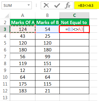
The succeeding image shows the marks of students A and B (columns A and B) in 10 subjects. The total marks of each subject are 200. We want to find those rows for which the marks of the two students are unequal. Use the “not equal to” signof Excel.

The steps to find if a difference exists between the two marks are listed as follows:

Step 1: In cell C3, type the “equal to” symbol followed by the cell reference B3. Since the difference between cells B3 and A3 needs to be assessed, insert the “not equal to” sign between these two cell references.

The formula should look like the expression “=B3<>A3.” This expression is also known as a statement or a condition.

Note: A condition in Excel is an expression that evaluates to either true or false. At a given time, a condition cannot be assessed as both true and false.

Step 2: Press the “Enter” key. The output in cell C3 is “true.” This is shown in the following image.

Step 3: Drag the formula of cell C3 till cell C12 by using the fill handle. This is shown in the following image.

Step 4: The outputs for the entire column C are shown in the following image. The outputs which are false have been colored yellow. The inferences from this dataset are stated as follows:

If the output is “true,” the values of column A and column B for a given row are not equal. This means that the “not equal to” excel condition for that particular row is met. For instance, the “not equal to” condition for row 3 is “=B3<>A3.” In other words, 124 is not equal to 54.
If the output is “false,” the values of column A and column B for a given row are equal. This means that the “not equal to” condition for that particular row is not met. For instance, the “not equal to” condition for row 5 is “=B5<>A5.” In other words, 120 is certainly equal to 120.

Overall, for three rows (rows 5, 6, and 10), the marks of students A and B are equal. Except for these rows, the marks are unequal in all the remaining rows (rows 3, 4, 7, 8, 9, 11, and 12). Without knowing the magnitude of difference, one cannot conclude whose performance (from students A and B) is better.

Example #2–Compare two Textual Values with the “Not Equal To” Operator

In the dataset of example #1, we have substituted random grades (from A to J) in place of numbers. We want to find the rows for which the grades of students A and B are unequal. Use the “not equal to” operator of Excel.

The steps to find if a difference exists (between the grades) are listed as follows:

Step 1: Enter the formula “=B3<>A3” in cell C3. Press the “Enter” key. The output in cell C3 is “true.” So, for row 3, the “not equal to” excel operator has validated that the values in the first and second cell (A3 and B3) are not equal.

Step 2: Drag the formula of cell C3 till cell C12. The outputs for the entire column C are shown in the following image. The single false output has been colored yellow.

The output in cell C3 meets the “not equal to” excel condition, which is “=B3<>A3.” In contrast, the output in cell C11 does not meet the “not equal to” condition, which is “=B11<>A11.” Hence, the grades of all rows, except row 11, are unequal. The grades of the two students are equal for row 11.

Example #3–Obtain Defined Results with the IF Function and the “Not Equal To” Condition

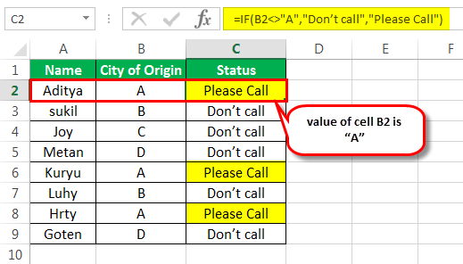
The succeeding image shows the names of a few candidates and their native places in columns A and B respectively. From these candidates, an organization wants to hire those candidates whose city of origin is “A.”

We want to differentiate candidates who need to be contacted and who need not be contacted for the further hiring process. For this, display the status as either “please call” or “don’t call” (in column C), depending on whether the hometown of a candidate is “A” or not.

Use the IF function and the “not equal to” operator of Excel.

The steps to use the IF functionIF function in Excel evaluates whether a given condition is met and returns a value depending on whether the result is “true” or “false”. It is a conditional function of Excel, which returns the result based on the fulfillment or non-fulfillment of the given criteria.
read more and the “not equal to” operator are listed as follows:

Step 1: Enter the following formula in cell C2.

“=IF(B2<>”A”,”Don’t call”,”Please Call”)”

Press the “Enter” key. Drag the formula till cell C9. The outputs of column C are shown in the succeeding image. The candidates whose city of origin is “A” have been assigned the “please call” status in column C.

Note: In the given IF formula, the condition [B2<>“A”] is the logical test. The string “don’t call” is “value_if_true” and the string “please call” is “value_if_false.”

So, the IF formula returns “don’t” call” for a given row, if the value of column B is not equal to “A” (i.e., the condition is true). It returns “please call” for a given row, if the value of column B is equal to “A” (i.e., the condition is false).

With the help of the IF function, Excel can display different results for the matched and unmatched conditions. For more details related to the IF function of Excel, click the hyperlink given immediately before step 1 of this example.

Step 2: The candidates whose hometown is other than “A” have been assigned the “don’t call” status in column C. This is shown in the following image.

Hence, only candidates “Aditya,” “Kuryu,” and “Hrty” should be called for the further round of interviews. The remaining candidates need not be contacted.

So, with the IF function and the “not equal to” excel operator, we have successfully differentiated the candidates who can be hired from those who cannot be hired.

Note: Notice that this step has been added only for the purpose of understanding. The preceding step (step 1) is complete in itself for the given task of hiring candidates.

Example #4–Count Specific Cells with the COUNTIF Function and the “Not Equal To” Condition

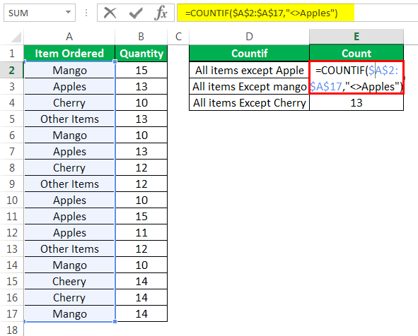
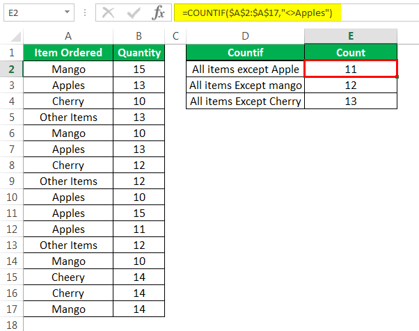
The succeeding image shows certain fruits (or items) in column A and their quantities ordered in column B. Apart from apples, mangoes, and cherries, the remaining fruits have been clubbed under “other items” in column A.

We want to count the number of cells (of column A) that are not equal to:

“Apples”
“Mango”
“Cherry”

There should be three outputs, one output excluding one fruit. Use the COUNTIF function and the “not equal to” operator of Excel.

The steps to use the COUNTIF functionThe COUNTIF function in Excel counts the number of cells within a range based on pre-defined criteria. It is used to count cells that include dates, numbers, or text. For example, COUNTIF(A1:A10,”Trump”) will count the number of cells within the range A1:A10 that contain the text “Trump”
read more and the “not equal to” operator are listed as follows:

Step 1: Enter the following formulas in cells E2, E3, and E4 respectively.

“=COUNTIF($A$2:$A$17,”<>Apples”)”
“=COUNTIF($A$2:$A$17,”<>Mango”)”
“=COUNTIF($A$2:$A$17,”<>Cherry”)”

Press the “Enter” key after entering each formula.

The first formula counts the number of cells in the range A2:A17, which do not contain the string “apples.” Likewise, the second formula counts the number of cells in this range that do not contain the string “mango.” The third formula helps count the number of cells in the given range (A2:A7), which do not contain the string “cherry.”

Notice that the succeeding image shows the formula in cell E2 and the result of the third formula in cell E4.

Note: “$A$2:$A$17” is the “range” argument of the preceding COUNTIF formulas. The condition “<>Apples” is the “criteria” argument of the first formula. In all the preceding formulas, the range is the same, but the criterions are different.

The COUNTIF counts the cells of a range, which satisfy a single criterion. For more details related to the COUNTIF function, click the hyperlink given before step 1 of this example.

Step 2: The following image shows the three outputs (in cells E2, E3, and E4) of the three formulas entered in the preceding step.

Notice that “cherry” has been deliberately misspelled as “cheery” in cell A15. As a result, this cell has also been counted (as a cell not containing “cherry”) by the third COUNTIF formula.

Had the word been correctly spelled in cell A15, the output in cell E4 would have been 12. In this case, cell A15 would have been excluded from the count (as a cell containing “cherry”).

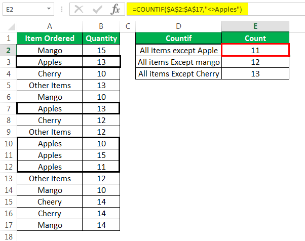
Step 3: The rows containing “apples” are displayed in black boxes in the following image. These rows are excluded while counting the cells not containing “apples.” Hence, 11 cells (in the range A2:A17) do not contain the string “apples.”

Likewise, in the given range, 12 cells do not contain the string “mango” and 13 cells do not contain the string “cherry.”

Note: This step has been added only for notifying the readers, the cells that are counted and the cells that are left out by the first COUNTIF formula (entered in step 1).

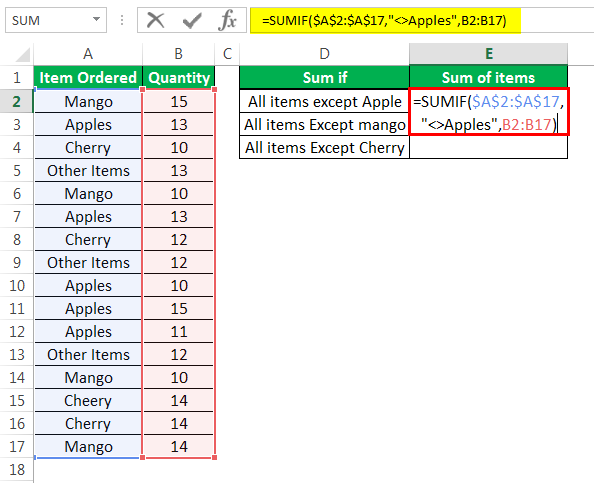
Example #5–Sum Particular Cells with the SUMIF Function and the “Not Equal To” Condition

Working on the data of example #3, we want to sum the quantities of column B that are not equal to:

“Apples”
“Mango”
“Cherry”

There should be three summed outputs where each output excludes one fruit. Use the SUMIF function and the “not equal to” sign of Excel.

The steps to use the SUMIF functionThe SUMIF Excel function calculates the sum of a range of cells based on given criteria. The criteria can include dates, numbers, and text. For example, the formula “=SUMIF(B1:B5, “<=12”)” adds the values in the cell range B1:B5, which are less than or equal to 12.
read more and the “not equal to” operator are listed as follows:

Step 1: Enter the following formulas in cells E2, E3, and E4 respectively.

“=SUMIF($A$2:$A$17,”<>Apples”,B2:B17)”
“=SUMIF($A$2:$A$17,”<>Mango”,B2:B17)”
“=SUMIF($A$2:$A$17,”<>Cherry”,B2:B17)”

The first formula is shown in the following image.

In all three formulas, the SUMIF function evaluates the range A2:A17. For cells not equal to “apples” (in range A2:A17), the first formula sums the numbers of the range B2:B17. Likewise, for cells not equal to “mango” in the given range (A2:A17), the second formula also sums the numbers of the range B2:B17. Similar summing is carried out by excluding cells containing “cherry.”

Note: “$A$2:$A$17” is the “range” argument of the SUMIF function. The condition “<>Apples” is the “criteria” argument. The range “B2:B17” is the “sum_range” argument of the SUMIF function.

With the SUMIF function, we have applied the given condition (in each formula) to the range A2:A17 and summed up the corresponding values of the range B2:B17. Usually, the SUMIF works with a single criterion. For more details related to the SUMIF function, click the hyperlink given before step 1 of this example.

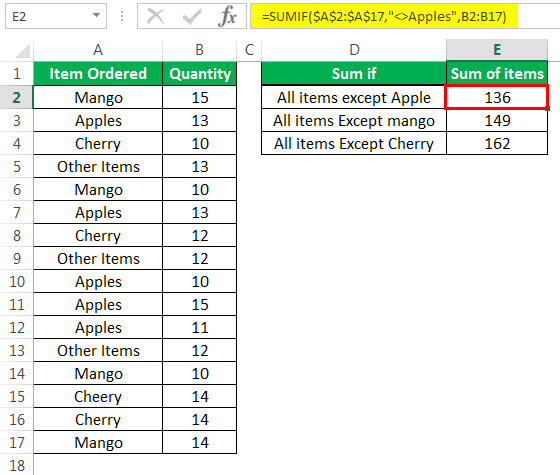
Step 2: Press the “Enter” key after entering each of the preceding formulas. The three summed outputs are shown in the following image.

Hence, the sum of all the fruit quantities except “apples” is 136. Excluding the cells containing “mango,” this sum is 149. Likewise, leaving the cells containing “cherry,” this sum is 162.

Notice that the value of cell B15 has also been included in the sum returned (in cell E4) by the third SUMIF formula (entered in step 1). This is because in cell A15, the spelling of “cherry” has been misspelled as “cheery.” Hence, Excel considers A15 as a cell not containing “cherry.”

The important points governing the usage of the “not equal to” operator of Excel are listed as follows:

The “not equal to” is the converse of the “equal to” operator. This implies that the interpretation of “true” and “false” is exactly the opposite with these two logical operators.
The results produced by the “not equal to” operator are similar to those returned by the NOT function of Excel. The NOT function reverses the “true” and “false” outcomes of a condition. For instance, if the output of a condition is “false,” the formula “=NOT(false)” returns “true.”
The “not equal to” operator is case-insensitive. This means that it ignores the casing of the two text strings that are compared. For instance, if “rose” and “ROSE” are compared using the “not equal to” operator, the output is “false.” This is because these two values mean the same to the “not equal to” excel operator.

Frequently Asked Questions

1. Define the “not equal to” operator and state how is it used in Excel.

The “not equal to” excel operator checks whether two values (numeric or textual) being compared are different from each other or not. If the values are different, the output is “true.” If the values are the same, the output is “false.” The “not equal to” operator is the easiest method to ensure that a difference exists between two values.

In Excel, the “not equal to” operator is used as follows:

“=value1<>value2”

“Value1” is the first value to be compared and “value2” is the second value to be compared.

Note: Exclude the beginning and ending double quotation marks while entering the “not equal to” condition in Excel. For more details related to the usage of this operator, refer to the examples of this article.

2. How to use the “not equal to” operator with the conditional formatting feature of Excel?

The steps to use the “not equal to” with the conditional formatting feature of Excel are listed as follows:

a. Select the range on which a conditional formatting rule is to be applied.
b. From the Home tab, click the “conditional formatting” drop-down from the “styles” group. Next, click “new rule.”
c. The “new formatting rule” window opens. Under “select a rule type,” choose the option “use a formula to determine which cells to format.”
d. Under “format values where this formula is true,” enter the desired formula. For instance, if cells (in the range A1:A6) not equal to 2 are to be formatted, enter the formula as “=A1<>2” (without the beginning and ending double quotation marks).
e. Click “format” and select a color from the “fill” tab. Click “Ok” in the “format cells” window.
f. Click “Ok” again in the “new formatting rule” window.

The chosen color (selected in step “e”) is applied to the selected range (selected in step “a”). If the formula given in step “d” is applied, the cells of the range A1:A6, which do not contain 2, are colored. No formatting is applied to the remaining cells.

Note: To conditionally format a range of text values by using the “not equal to” operator, keep the string of the formula in double quotation marks. For instance, the formula [=A1<>“rose”] formats those cells of the selected range which do not contain the string “rose.” Exclude the beginning and ending square brackets while applying this formula.

3. How to use the “not equal to” operator to find blanks in a range of Excel?

The steps to find blanks in Excel by using the “not equal to” operator are listed as follows:

a. Enter the formula containing the cell reference (to be evaluated), “not equal to” operator, and an empty text string. For instance, if blanks in the range A1:A6 are to be found, enter the formula =A1<>“” in cell B1.
b. Press the “Enter” key. Drag the formula to the remaining range (of column B) to obtain outputs for the entire column (column A).

The cells containing blanks have been identified. The formula entered in step “a” returns “true” for all values which are not blanks. For all blank values, this formula returns “false.”

Since the double quotation marks of the formula represent an empty string, a “false” implies that the cell value is equal to an empty string. Conversely, a “true” implies that the cell contains some value, which is not equal to an empty string.

Explanation

In this example, the goal is to count the number of cells in column D that are not equal to a given color. The simplest way to do this is with the COUNTIF function, as explained below.

Not equal to

In Excel, the operator for not equal to is «<>». For example:

=A1<>10 // A1 is not equal to 10
=A1<>"apple" // A1 is not equal to "apple"

COUNTIF function

The COUNTIF function counts the number of cells in a range that meet supplied criteria:

=COUNTIF(range,criteria)

To use the not equal to operator (<>) in COUNTIF, it must be enclosed in double quotes like this:

=COUNTIF(range,"<>10") // not equal to 10
=COUNTIF(range,"<>apple") // not equal to "apple"

This is a requirement of COUNTIF, which is in a group of eight functions that share this syntax. In example shown, we want to count cells not equal to «red» in D5:D16, so we use «<>red» for criteria. The formula in G5 is:

=COUNTIF(D5:D16,"<>red") // returns 9

In cell G6, we count all cells not equal to blue with a similar formula:

=COUNTIF(D5:D16,"<>blue") // returns 7

Note: COUNTIF is not case-sensitive. The word «red» can appear in any combination of uppercase / lowercase letters.

Not equal to another cell

To use a value in another cell as part of the criteria, use the ampersand (&) operator to concatenate like this:

=COUNTIF(range,"<>"&A1)

For example, if A1 contains 100 the criteria will be «<>100» after concatenation, and COUNTIF will count cells not equal to 100:

=COUNTIF(range,"<>100")

COUNTIFS function

The COUNTIFs function is designed to handle multiple criteria, but can be used just like the COUNTIF function in this example:

=COUNTIFS(D5:D16,"<>red") // returns 9
=COUNTIFS(D5:D16,"<>blue") // returns 7

Video: How to use the COUNTIFS function

Источник

Excel Not Equal To (Table of Contents)

Not Equal To in Excel
How to Put ‘ Not Equal To ‘ in Excel?

Not Equal To in Excel

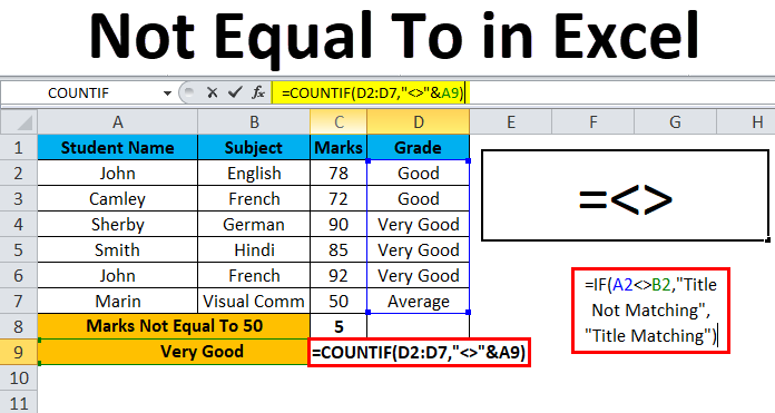
Not Equal To generally is represented by striking equal sign when the values are not equal to each other. But in Excel, it is represented by greater than and less than operator sign “<>” between the values which we want to compare. If the values are equal, then it used the operator will return as TRUE, else we will get FALSE. We can use the Not Equal operator along with other conditional functions as IF, SUMIF, COUNTIF function to get some other kind of meaning of results.

How to Put ‘ Not Equal To ‘ in Excel?

Not Equal To in Excel is very simple and easy to use. Let’s understand the working of Not Equal To Operator in Excel by some examples.

You can download this Not Equal To Excel Template here – Not Equal To Excel Template

Example #1 – Using ‘ Not Equal To Excel ‘ Operator

In this example, we are going to see how to use the Not Equal To logical operation <> in excel.

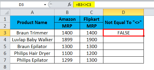
Consider the below example, which has values in both the columns now; we are going to check the Brand MRP of Amazon and Flipkart.

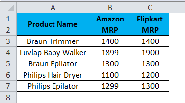
Now we are going to check that Amazon MRP is not equal to Flipkart MRP by following the below steps.

Create a new column.

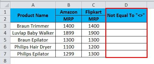
Apply the formula in excel as shown below.

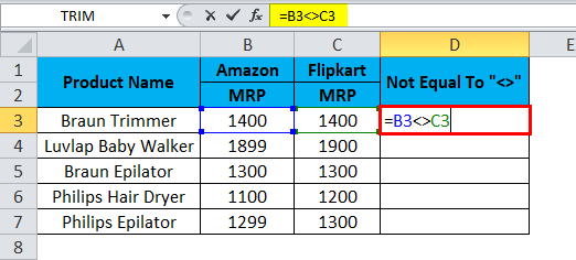
So as we can see in the above screenshot, we applied the formula as =B3<>C3 here, we can see that in the B3 column Amazon MRP is 1400, and Flipkart MRP is 1400, so the MRP matches exactly.
Excel will check if B3 values are not equal to C3, then it returns TRUE or else it will return FALSE.
Here in the above screenshot, we can see that Amazon MRP is equal to Flipkart MRP, so we will get the output as FALSE, which is shown in the below screenshot.

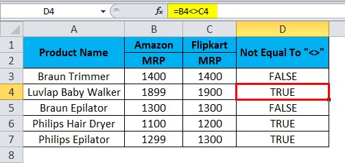
Drag down the formula for the next cell. So the output will be as below:

We can see that the formula =B4<>C4; in this case, Amazon MRP is not equal to Flipkart MRP. So excel will return the output as TRUE, as shown below.

Example #2 – Using String

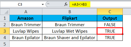
In this excel example, we are going to see how not equal to excel operator works in strings. Consider the below example, which shows two different titles named for Amazon and Flipkart.

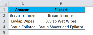
Here we will check that Amazon’s title name matches the Flipkart title name by following the below steps.

First, create a new column called Output.

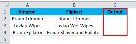
Apply the formula as =A2<>B2.

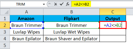
So the above formula will check for A2 title name is not equal to B2 title name if it is not equal, it will return FALSE or else it will return TRUE as we can see that both the title names are the same and it will return the output as FALSE which is shown in the below screenshot.

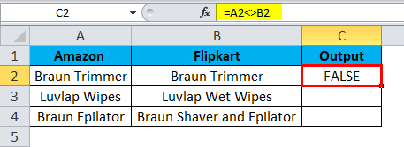
Drag down the same formula for the next cell. So the output will be as below:

As =A3<>B3, where we can see the A3 title is not equal to the B3 title, so we will get the output as TRUE which is shown as the output in the below screenshot.

Example #3 – Using IF Statement

In this excel example, we are going to see how to use the if statement in the Not Equal To operator.

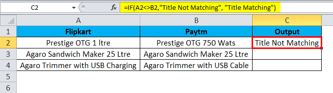
Consider the below example, where we have title names of both Flipkart and Paytm, as shown below.

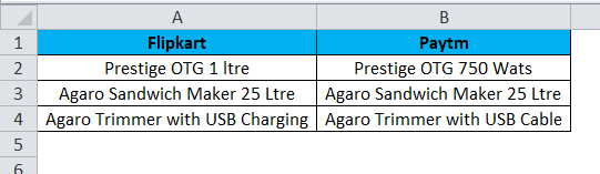
Now we are going to apply the Not Equal To Excel operator inside the if statement to check both the title names are equal or not equal by following the below steps.

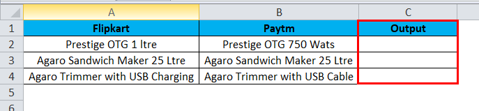
Create a new column as Output.

Now apply the if condition statement as follows =IF(A2<>B2, “Title Not Matching”, “Title Matching”)

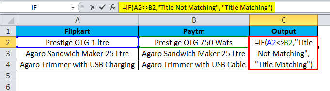
Here in the if condition, we used not equal to Operator to check whether the title is equal to or not equal.
Moreover, we have mentioned in the if condition in double-quotes as “Title Not Matching”, i.e., if it is not equal to it, it will return as “Title Not Matching”, or else it will return “Title Matching”, as shown in the below screenshot.
As we can see that both the title names are different, and it will return the output as Title Not Matching which is shown in the below screenshot.

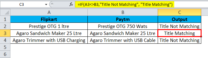
Drag down the same formula for the next cell.

In this example, we can see that the A3 title is equal to the B3 title; hence we will get the output as “Title Matching “, which is shown as the output in the below screenshot.

Example #4 – Using the COUNTIF Function

In this excel example, we are going to see how the COUNTIF Function works in the Not Equal To operator.

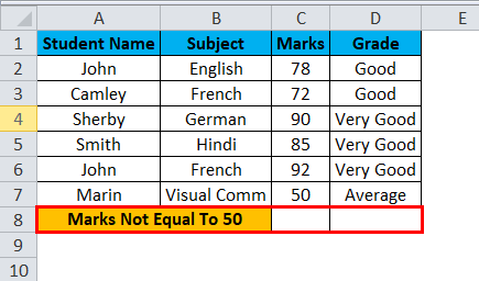
Consider the below example, which shows student’s subject marks along with the grade.

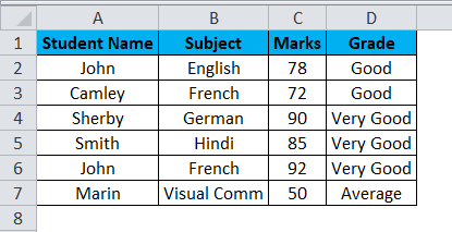
Here we are going to count how many students have taken the marks in it equal to 94 by following the below steps.

Create a new row named as Marks Not Equal To 50.

Now apply the COUNTIF formula as =COUNTIF(C2:C7,”<>50″)

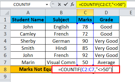
As we can see in the above screenshot, we have applied the COUNTIF function to find out Student marks not equal to 50. We have selected the cells C2:C7, and in the double quotes, we have used <> not equal to Operator and mentioned the number 50.
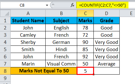
The above formula counts the student’s marks which is not equal to 50, and return the output as 5, as shown in the below result.
In the below screenshot, we can see that marks not equal to 50 are 5, i.e. Five students scored marks more than 50.

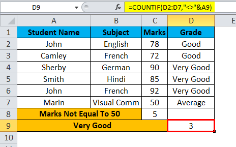
Now we will use a string to check the student’s grade stating how many students are not equal to the grade “Very Good”, which is shown in the below screenshot.

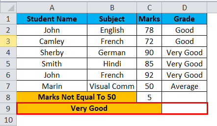
For this, we can apply the formula as =COUNTIF(D2:D7,”<>”& A9).

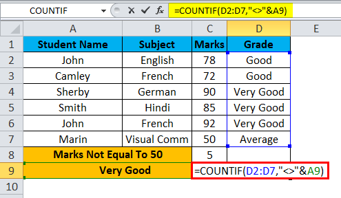
So this COUNTIF function will find the student’s grade from the range we have specified D2:D7 using the Not Equal To Excel OPERATOR. The grade variable “VERY GOOD” has been concatenated by the operator “&” by specifying A9. Which will give us the result of 3, i.e. 3 students grade are not equal to “Very Good” which is shown in the below output.

Things to Remember About Not Equal To in Excel

In Microsoft excel, logical operators mostly used in conditional formatting, which will give us the perfect result.
Not Equal To operator always requires at least two values to check either it is “TRUE” or “FALSE”.
Make sure that you are giving the correct condition statement while using the Not Equal To the operator, or else we will get an invalid result.

What’s Wrong With Excel?

I try to get on the Mr. Excel forums a few times a week and this question is one of the most popular troubleshooting questions posted. This is quite understandable as humans tremendously excel at processing visually. For example, if we see two red apples sitting on a table we can immediately process the texture, approximate weight, and even the taste of those two objects from a fairly good distance. And because they are both apples we immediately assume these properties are the same for both. This is all due to their similar appearance. But what if you opened up one of those apples and it looked like this:

Source: www.nacentralohio.com/gmo-truths-and-consequences/gmo-appleorange/

Not what you were expecting, right? The main point I want to get across to you today is things might not always be as they appear in Excel. The only way to find out is to cut in and see what’s inside! Below I will list a series of tests you can perform on your values to determine why Excel thinks data points are different when they appear to be the same.

Spaces Before or After Your Values

Sometimes when you receive extracted data or you are trying to compare two data sets, ‘ghost’ characters will slip into the cell values and try to play tricks with you. These ‘ghost’ characters take form as spaces and if they occur in the beginning or end of text, we cannot see any visual evidence of their existence! In the example below, Cell C2 is testing to see if A2 = B2. This text is giving us a FALSE which means they do not equal each other. What is causing this ? Both cells have just the word ‘Hello’ in them! Well, if you use the LEN( ) function to determine the length (how many characters) of our ‘Hello’ values, you will see that Value 1 has a length of 5 and Value 2 has a length of 6. This is because there was an extra space entered in Cell B2. Cell B2’s real value is «Hello «.

EExcel says numbers or text not found or equal

How Can We Handle This?

Well, Excel has a function called TRIM. What TRIM does is remove all spaces before and after a text string (it ignores spaces in between words). You can see below if we include TRIM in our test we will output a TRUE value.

Excel says numbers or text not found or equal

Use The TRIM Function With LOOKUP Functions

You will most often run into this problem when using Lookup Functions (ie VLOOKUP, MATCH, HLOOKUP, etc…). If you run into a situation where you believe your VLOOKUP should be finding a match, try wrapping a TRIM function around your lookup value. An example formula could look like this:

=VLOOKUP(TRIM(A2), $D$2:$Z$400, 3, FALSE)

Text versus Numerical

Another very popular situation that arises when exporting numerical data from outside databases is mismatching data formats. I find this occurs most often with identification values where your data may have leading zeroes (such as employee IDs or Invoice numbers). In our example below we have two cells containing the value of 200….or so it seems! As you can see by the test in Cell C2, Cells A2 and B2 do not equal each other. For your test in this situation, you can use the ISNUMBER function to, yep you guessed it, test if your cell values are numerical.

So how can we handle this?

To force a text string to become a numerical value you can use the VALUE function. By incorporating the VALUE function in your test you can see (below) the test will successfully compare the two numbers as equal.

Use The VALUE Function With LOOKUP Functions

Similar to how you can use TRIM within a lookup function to cleanup your data, you can also use VALUE in the same fashion with your lookup functions. An example formula may look like this:

=VLOOKUP(VALUE(A2), $D$2:$Z$400, 3, FALSE)

Convert Text Into Values

Another option could be to convert all the text values to numerical ones. If Excel notices a text value that only has numbers in it, the cell will get flagged. If you look very carefully in the above two images (click on them to enlarge), you can see a green indicator in the upper left-hand corner of Cell B2. To convert this cell’s value into a numerical one do the following:

Select the cell(s) with the green indicator (a little box should appear with a drop down arrow next to the first cell selected)
Click the drop down arrow
Select Convert to Number
Excel with cycle through your selection and convert all your text values to numerical ones (WARNING: with large data sets this will take some time, this is usually a good time to schedule a coffee break)

Convert text to number dialog

An Impossible Value

Another scenario I wanted to throw into this post deals with impossible values. More specifically, this can occur with dates users enter in manually. In the example below, Cell C2 is attempting to subtract the two dates in Cell A2 and Cell B2. Only…when the operation is calculated, a #Value! error occurs. This error is being caused by the fact there are not 31 days in the month of April. We can tell this by using the DAY function. The DAY function ouputs the number of days in a date value. Since April 31st is not a possible date value, an error occurs (see Cell B3 below).

Excel says numbers or text not found or equal

How Do You Prevent This?

My recommendation to prevent any input errors is to use Excel’s Data Validation feature. This feature is located within the Data tab of the Ribbon, inside the Data Tools group. If you are trying to prevent users from incorrectly entering in data following a pattern, you can check out my post covering How To Validate Patterns in Excel.

Data Validation Menu in Excel Ribbon

How Do You Handle Your Data?

In this post I described three scenarios I run into all the time while working with data exports from third-party database software. I am sure there are other scenarios I overlooked and I want to know if you have come across any other scenarios where Excel messes with your eyes! I look forward to hearing about your painful data experiences!

About The Author

Hey there! I’m Chris and I run TheSpreadsheetGuru website in my spare time. By day, I’m actually a finance professional who relies on Microsoft Excel quite heavily in the corporate world. I love taking the things I learn in the “real world” and sharing them with everyone here on this site so that you too can become a spreadsheet guru at your company.

Through my years in the corporate world, I’ve been able to pick up on opportunities to make working with Excel better and have built a variety of Excel add-ins, from inserting tickmark symbols to automating copy/pasting from Excel to PowerPoint. If you’d like to keep up to date with the latest Excel news and directly get emailed the most meaningful Excel tips I’ve learned over the years, you can sign up for my free newsletters. I hope I was able to provide you with some value today and I hope to see you back here soon!

— Chris
Founder, TheSpreadsheetGuru.com

Источник

What is “Not Equal To” Sign in Excel?

Table of contents

How is the “Not Equal To” Sign Used in Excel?

Example #1–Compare two Numeric Values with the “Not Equal To” Operator

Example #2–Compare two Textual Values with the “Not Equal To” Operator

Example #3–Obtain Defined Results with the IF Function and the “Not Equal To” Condition

Example #4–Count Specific Cells with the COUNTIF Function and the “Not Equal To” Condition

Example #5–Sum Particular Cells with the SUMIF Function and the “Not Equal To” Condition

Frequently Asked Questions

Recommended Articles

Explanation

Not equal to

COUNTIF function

Not equal to another cell

COUNTIFS function

Not Equal To in Excel

How to Put ‘ Not Equal To ‘ in Excel?

Example #1 – Using ‘ Not Equal To Excel ‘ Operator

Example #2 – Using String

Example #3 – Using IF Statement

Example #4 – Using the COUNTIF Function

Things to Remember About Not Equal To in Excel

Recommended Articles

What’s Wrong With Excel?

Spaces Before or After Your Values

How Can We Handle This?

Use The TRIM Function With LOOKUP Functions

Text versus Numerical

So how can we handle this?

Use The VALUE Function With LOOKUP Functions

Convert Text Into Values

An Impossible Value

How Do You Prevent This?

How Do You Handle Your Data?

About The Author