Excel drop down list with values - Word и Excel - помощь в работе с программами

A drop-down list means that one cell includes several values. When the user clicks the arrow on the right, a certain scroll appears. He can choose a specific one.

A drop-down list is a very handy Excel tool for checking the entered data. The following features of drop-down lists allow you to increase the convenience of data handling: data substitution, displaying data from another sheet or file, the presence of the search and dependency function.

Creating a drop-down list

Path: the «DATA» menu – the «Data Validation» tool – the «Settings» tab. The data type – «List».

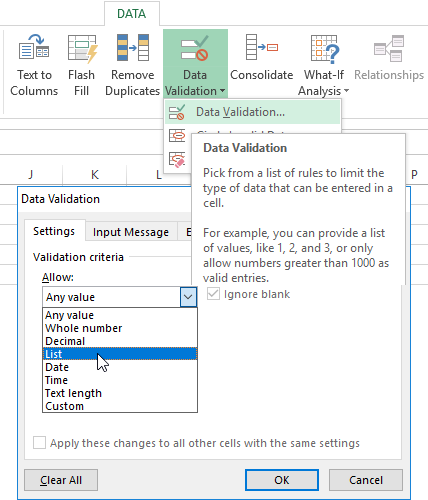
You can enter the values from which the drop-down list will consist, in different ways:

Manually through the «Comma» in the «Source:» field.

Comma.

Enter the values in advance. Specify a range of cells with a list as a source.

Assign a name for a range of values and enter the name in the «Source:» field.

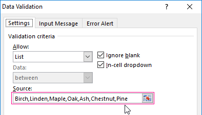
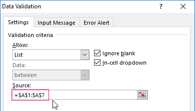
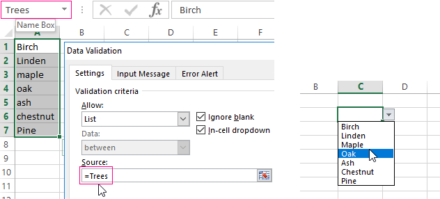
Any of the mentioned options will give the same result.

Drop-down list with data lookup in Excel

It is necessary to make a drop-down list with values from the dynamic range. If changes are made to the available range (data are added or deleted), they are automatically reflected in the drop-down list.

Highlight the range for the drop-down list. Find the «Format As Table» tool in the main menu.

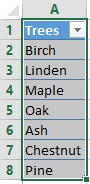
The styles will open. Choose any of them. For solving our task, design does not matter. The presence of the header is important. In our example, the header is cell A1 with the word «Trees». That is, you need to select a table style with a header row. You’ll get the following range:

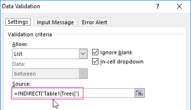
Put the cursor on the cell where the drop-down list will be located. Open the parameters of the «Data Validation» tool (the path is described above). In the «Source:» field, write the following function:

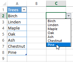
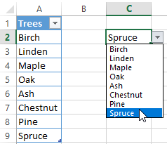
Let’s test it. Here is our table with a list on one sheet:

Add the new value «Spruce» to the table.

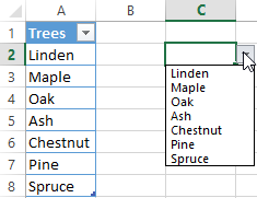
Now delete the «Birch» value.

delete.

The «smart table», which easily «expands» and changes, has helped us to perform our task.

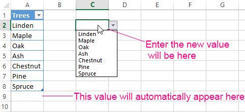
Now let’s make it possible to enter new values directly into the cell with this list and have data automatically added to the range.

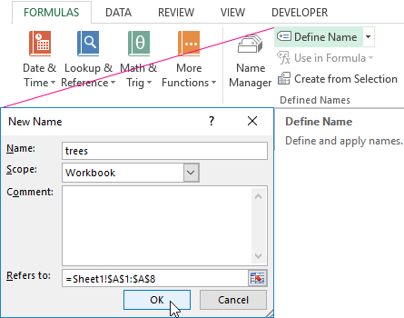
Form a named range. Path: «FORMULAS» — «Define Name» — «New Name». Enter a unique name for the range and press OK.

Create a drop-down list in any cell. You already know how to do this. Source – name range: =trees.
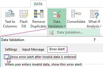
Clear the following check boxes: «Error Alert», «Show error alert invalid data entered». If you do not do this, Excel will not allow you to enter new values.

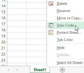
Launch the Visual Basic Editor. To do this, right-click on the name of the sheet and go to the «View Code» tab. Alternatively, press Alt + F11 simultaneously. Copy the code (just insert your parameters).

Private Sub Worksheet_Change(ByVal Target As Range) Dim lReply As Long If Target.Cells.Count > 1 Then Exit Sub If Target.Address = "$C$2" Then If IsEmpty(Target) Then Exit Sub If WorksheetFunction.CountIf(Range("trees"), Target) = 0 Then lReply = MsgBox("Add entered name " & _ Target & " in the drop-down list?", vbYesNo + vbQuestion) If lReply = vbYes Then Range("trees").Cells(Range("trees").Rows.Count + 1, 1) = Target End If End If End If End Sub

Save it, setting the «Excel Macro-Enabled Workbook» file type.

When you enter a new name in the empty cell of the drop-down list, the following message will appear: «Add entered name Baobab?».

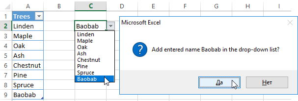
Click «OK» and one more row with the «Baobab» value will be added.

Excel drop-down list with data from another sheet / file

When the values for the drop-down list are located on another sheet or in another workbook, the standard method does not work. You can solve the problem with the help of the =INDIRECT() function: it will form the correct link to an external source of information.

Activate the cell where we want to put the drop-down menu.
Open the Data Validation options. In the «Source:» field, enter the following formula:

The name of the file from which the information for the list is taken is enclosed in square brackets. This file must be opened. If the book with the desired values is stored in a different folder, you need to specify the path completely.

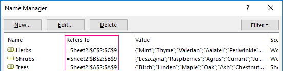
How to create dependent drop-down lists

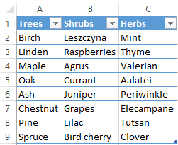
Take three named ranges:

It is an indispensable prerequisite. Above you can see how to turn a normal scroll in a named range (using the «Name Manager»). Remember that the name cannot contain spaces or punctuation.

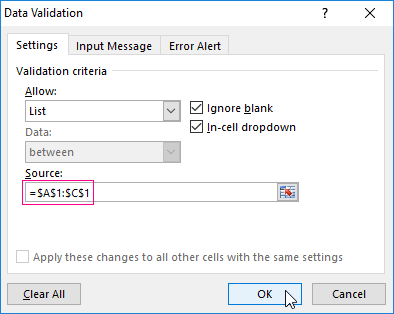
Create the first drop-down list, which will include the names of the ranges.

Having placed the cursor on the «Source:» field, go to the sheet and select the required cells alternately.

Source.

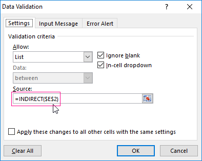
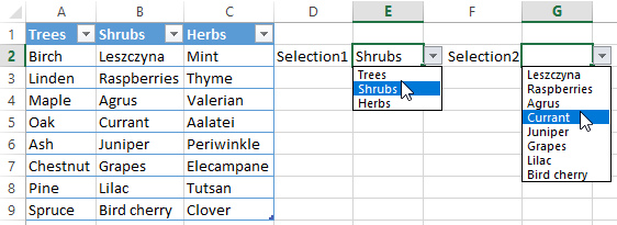
Now create the second drop-down menu. It should reflect those words that correspond to the name chosen in the first scroll. If the «Trees», then «Linden», «Maple», etc. should correspond to it. Enter the following function: =INDIRECT(А1) in the «Source:» field. A1 is a cell with the first range.

Selecting multiple values from a drop-down list in Excel

Sometimes, you need to select several items from the drop-down list. Let’s consider the ways of performing this task.

Create a standard ComboBox using the «Data Validation» tool. Add a ready-made macro to the sheet module. The way how to do this is described above. With its help, the selected values will be added to the right of the drop-down menu.

Private Sub Worksheet_Change(ByVal Target As Range) On Error Resume Next If Not Intersect(Target, Range("E2:E9")) Is Nothing And Target.Cells.Count = 1 Then Application.EnableEvents = False If Len(Target.Offset(0, 1)) = 0 Then Target.Offset(0, 1) = Target Else Target.End(xlToRight).Offset(0, 1) = Target End If Target.ClearContents Application.EnableEvents = True End If End Sub

For the selected values to be shown from below, insert another code for processing.

Private Sub Worksheet_Change(ByVal Target As Range) On Error Resume Next If Not Intersect(Target, Range("H2:K2")) Is Nothing And Target.Cells.Count = 1 Then Application.EnableEvents = False If Len(Target.Offset(1, 0)) = 0 Then Target.Offset(1, 0) = Target Else Target.End(xlDown).Offset(1, 0) = Target End If Target.ClearContents Application.EnableEvents = True End If End Sub

For the selected values to be displayed in the same cell separated by any punctuation mark, apply this module.

Private Sub Worksheet_Change(ByVal Target As Range) On Error Resume Next If Not Intersect(Target, Range("C2:C5")) Is Nothing And Target.Cells.Count = 1 Then Application.EnableEvents = False newVal = Target Application.Undo oldval = Target If Len(oldval) <> 0 And oldval <> newVal Then Target = Target & "," & newVal Else Target = newVal End If If Len(newVal) = 0 Then Target.ClearContents Application.EnableEvents = True End If End Sub

Do not forget to change the ranges to «your own» ones. Create scroll in the classical way. The rest of the work will be done by macros.

Searchable drop-down list in Excel

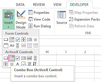
On the «DEVELOPER» tab find the «Insert» tool – «ActiveX». Here you need the button «Combo Box (ActiveX Control)» (focus your attention on the tooltips).

Click on the icon – «Design Mode» becomes active. Draw a small rectangle (the place of the future scroll) with a cursor that transforms to a «cross».

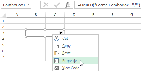
Click «Properties» to open a Combobox1 of settings.

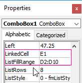
Enter the range in the ListFillRange row (manually). The cell where the selected value will be displayed can be changed in the LinkedCell row. Changing of the font and size can be done in Font row.

Download drop-down lists example

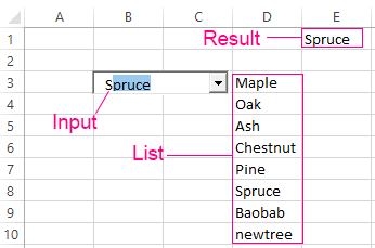
When you enter the first letters from the keyboard, the appropriate items are displayed. These are not all the pleasant moments of this instrument. Here you can customize the visual representation of information, specify two columns at once as a source.

Источник

Содержание

0.1 Простейший способ
- 0.1.1 Excel
- 0.1.2 Calc
0.2 Простейший способ
- 0.2.1 Excel
- 0.2.2 Calc
0.3 Мудрейший способ
- 0.3.1 Excel
- 0.3.2 Calc
- 0.3.3 Кстати

1 , но можно и «неформально» обрамить его тэгом — и покажи мне разницу…«, но имеет место бывать. Выделите ячейки с данными, которые должны попасть в выпадающий список (например, наименованиями товаров). Выберите в меню Вставка — Имя — Присвоить (Insert — Name — Define) и введите имя (можно любое, но обязательно без пробелов!) для выделенного диапазона (например Товары). Нажмите ОК. Можно сделать и так: Выделить диапазон ячеек (А1, В1, С1 в данном примере), и претворить его в «реальный» список В любом случае списку должно быть присвоено уникальное имя. Выделите ячейки (можно сразу несколько), в которых хотите получить выпадающий список и выберите в меню «Данные — Проверка» (Data — Validation). На первой вкладке «Параметры» из выпадающего списка «Тип данных» выберите вариант «Список» и введите в строчку «Источник» знак равно и имя диапазона (т.е. =Товары). Почему это круто: список «Товары» можно будет потом произвольно увеличивать или уменьшать. Табличный редактор будет учитывать не определенные ячейки, расположенные в определенном месте, а список as is. И все изменения в списке будут распространяться на все ячейки, которые «проверяют его для создания выпадающих списков». Горячие клавиши Курсор стоит на ячейке с выпадающим списком. Excel Alt+Down arrow. То есть, Alt+стрелка «вниз». Calc По-умолчанию не установлено. В справке написано Ctrl+D, но в справке баг (увы). Поэтому назначаем лично: Tools > Customize > Keyboard > Shortcut Keys Проскроллить и выбрать желаемое сочетание клавиш для открытия существующего списка. Я выбрал Ctrl+Down. Внимание, Alt+Down недоступно (вообще все сочетания с Alt тут недоступны для редактирования). В Functions > Category выбрать Edit. В Functions > Function выбрать Selection List. Нажать на кнопку Modify. Дополнение Всякие другие волшебства на тему выпадающих списков см. на Planeta Excel. Особенно «Ссылки по теме«. Прием комментариев к этой записи завершён. «Как зделать так чбо если в віпадающем списке нет нужного варианта я в ручную набираю в етой ячейке и оно автоматически добавляется в віпадающий список, и след раз уже там есть» — хз. Тут нам не то, и не это. Не надо задавать вопросы о том, как сделать ещё что-то с этими прекрасными выпадающими списками. Здесь даже не форум по Excel. Это блог о тестировании программного обеспечения. Вы же любите тестировать, правда?
Create a Drop-down List | Tips and Tricks Drop-down lists in Excel are helpful if you want to be sure that users select an item from a list, instead of typing their own values. Create a Drop-down List To create a drop-down list in Excel, execute the following steps. 1. On the second sheet, type the items you want to appear in the drop-down list. 2. On the first sheet, select cell B1. 3. On the Data tab, in the Data Tools group, click Data Validation. The ‘Data Validation’ dialog box appears. 4. In the Allow box, click List. 5. Click in the Source box and select the range A1:A3 on Sheet2. 6. Click OK. Result: Note: if you don’t want users to access the items on Sheet2, you can hide Sheet2. To achieve this, right click on the sheet tab of Sheet2 and click on Hide. Tips and Tricks Below you can find a few tips and tricks when creating drop-down lists in Excel. 1. You can also type the items directly into the Source box, instead of using a range reference. Note: this makes your drop-down list case sensitive. For example, if a user types pizza, an error alert will be displayed. 2a. If you type a value that is not in the list, Excel shows an error alert. 2b. To allow other entries, on the Error Alert tab, uncheck ‘Show error alert after invalid data is entered’. 3. To automatically update the drop-down-list, when you add an item to the list on Sheet2, use the following formula: =OFFSET(Sheet2!$A$1,0,0,COUNTA(Sheet2!$A:$A),1) Explanation: the OFFSET function takes 5 arguments. Reference: Sheet2!$A$1, rows to offset: 0, columns to offset: 0, height: COUNTA(Sheet2!$A:$A), width: 1. COUNTA(Sheet2!$A:$A) counts the number of values in column A on Sheet2 that are not empty. When you add an item to the list on Sheet2, COUNTA(Sheet2!$A:$A) increases. As a result, the range returned by the OFFSET function expands and the drop-down list will be updated. 4. Do you want to take your Excel skills to the next level? Learn how to create dependent drop-down lists in Excel.
A drop-down list is an excellent way to give the user an option to select from a pre-defined list. It can be used while getting a user to fill a form, or while creating interactive Excel dashboards. Drop-down lists are quite common on websites/apps and are very intuitive for the user. Watch Video – Creating a Drop Down List in Excel In this tutorial, you’ll learn how to create a drop down list in Excel (it takes only a few seconds to do this) along with all the awesome stuff you can do with it. How to Create a Drop Down List in Excel In this section, you will learn the exacts steps to create an Excel drop-down list: Using Data from Cells. Entering Data Manually. Using the OFFSET formula. #1 Using Data from Cells Let’s say you have a list of items as shown below: Here are the steps to create an Excel Drop Down List: Select a cell where you want to create the drop down list. Go to Data –> Data Tools –> Data Validation. In the Data Validation dialogue box, within the Settings tab, select List as the Validation criteria. As soon as you select List, the source field appears. In the source field, enter =$A$2:$A$6, or simply click in the Source field and select the cells using the mouse and click OK. This will insert a drop down list in cell C2. Make sure that the In-cell dropdown option is checked (which is checked by default). If this option in unchecked, the cell does not show a drop down, however, you can manually enter the values in the list. Note: If you want to create drop down lists in multiple cells at one go, select all the cells where you want to create it and then follow the above steps. Make sure that the cell references are absolute (such as $A$2) and not relative (such as A2, or A$2, or $A2). #2 By Entering Data Manually In the above example, cell references are used in the Source field. You can also add items directly by entering it manually in the source field. For example, let’s say you want to show two options, Yes and No, in the drop down in a cell. Here is how you can directly enter it in the data validation source field: This will create a drop-down list in the selected cell. All the items listed in the source field, separated by a comma, are listed in different lines in the drop down menu. All the items entered in the source field, separated by a comma, are displayed in different lines in the drop down list. Note: If you want to create drop down lists in multiple cells at one go, select all the cells where you want to create it and then follow the above steps. #3 Using Excel Formulas Apart from selecting from cells and entering data manually, you can also use a formula in the source field to create an Excel drop down list. Any formula that returns a list of values can be used to create a drop-down list in Excel. For example, suppose you have the data set as shown below: Here are the steps to create an Excel drop down list using the OFFSET function: This will create a drop-down list that lists all the fruit names (as shown below). Note: If you want to create a drop-down list in multiple cells at one go, select all the cells where you want to create it and then follow the above steps. Make sure that the cell references are absolute (such as $A$2) and not relative (such as A2, or A$2, or $A2). How this formula Works?? In the above case, we used an OFFSET function to create the drop down list. It returns a list of items from the ra It returns a list of items from the range A2:A6. Here is the syntax of the OFFSET function: =OFFSET(reference, rows, cols, , ) It takes five arguments, where we specified the reference as A2 (the starting point of the list). Rows/Cols are specified as 0 as we don’t want to offset the reference cell. Height is specified as 5 as there are five elements in the list. Now, when you use this formula, it returns an array that has the list of the five fruits in A2:A6. Note that if you enter the formula in a cell, select it and press F9, you would see that it returns an array of the fruit names. Creating a Dynamic Drop Down List in Excel (Using OFFSET) The above technique of using a formula to create a drop down list can be extended to create a dynamic drop down list as well. If you use the OFFSET function, as shown above, even if you add more items to the list, the drop down would not update automatically. You will have to manually update it each time you change the list. Here is a way to make it dynamic (and it’s nothing but a minor tweak in the formula): Select a cell where you want to create the drop down list (cell C2 in this example). Go to Data –> Data Tools –> Data Validation. In the Data Validation dialogue box, within the Settings tab, select List as the Validation criteria. As soon as you select List, the source field appears. In the source field, enter the following formula: =OFFSET($A$2,0,0,COUNTIF($A$2:$A$100,””)) Make sure that the In-cell drop down option is checked. Click OK. In this formula, I have replaced the argument 5 with COUNTIF($A$2:$A$100,””). The COUNTIF function counts the non-blank cells in the range A2:A100. Hence, the OFFSET function adjusts itself to include all the non-blank cells. Note: For this to work, there must NOT be any blank cells in between the cells that are filled. If you want to create a drop-down list in multiple cells at one go, select all the cells where you want to create it and then follow the above steps. Make sure that the cell references are absolute (such as $A$2) and not relative (such as A2, or A$2, or $A2). Copy Pasting Drop-Down Lists in Excel You can copy paste the cells with data validation to other cells, and it will copy the data validation as well. For example, if you have a drop-down list in cell C2, and you want to apply it to C3:C6 as well, simply copy the cell C2 and paste it in C3:C6. This will copy the drop-down list and make it available in C3:C6 (along with the drop down, it will also copy the formatting). If you only want to copy the drop down and not the formatting, here are the steps: This will only copy the drop down and not the formatting of the copied cell. Caution while Working with Excel Drop Down List You need to to be careful when you are working with drop down lists in Excel. When you copy a cell (that does not contain a drop down list) over a cell that contains a drop down list, the drop down list is lost. The worst part of this is that Excel will not show any alert or prompt to let the user know that a drop down will be overwritten. How to Select All Cells that have a Drop Down List in it Sometimes, it ‘s hard to know which cells contain the drop down list. Hence, it makes sense to mark these cells by either giving it a distinct border or a background color. Instead of manually checking all the cells, there is a quick way to select all the cells that have drop-down lists (or any data validation rule) in it. This would instantly select all the cells that have a data validation rule applied to it (this includes drop down lists as well). Now you can simply format the cells (give a border or a background color) so that visually visible and you don’t accidentally copy another cell on it. Here is another technique by Jon Acampora you can use to always keep the drop down arrow icon visible. You can also see some ways to do this in this video by Mr. Excel. Creating a Dependent / Conditional Excel Drop Down List Here is a video on how to create a dependent drop-down list in Excel. If you prefer reading over watching a video, keep reading. Sometimes, you may have more than one drop-down list and you want the items displayed in the second drop down to be dependent on what the user selected in the first drop-down. These are called dependent or conditional drop down lists. Below is an example of a conditional/dependent drop down list: In the above example, when the items listed in ‘Drop Down 2’ are dependent on the selection made in ‘Drop Down 1’. Now let’s see how to create this. Here are the steps to create a dependent / conditional drop down list in Excel: Now, when you make the selection in Drop Down 1, the options listed in Drop Down List 2 would automatically update. Download the Example File How does this work? – The conditional drop down list (in cell E3) refers to =INDIRECT(D3). This means that when you select ‘Fruits’ in cell D3, the drop down list in E3 refers to the named range ‘Fruits’ (through the INDIRECT function) and hence lists all the items in that category. Important Note While Working with Conditional Drop Down Lists in Excel: When you have made the selection, and then you change the parent drop down, the dependent drop down would not change and would, therefore, be a wrong entry. For example, if you select the US as the country and then select Florida as the state, and then go back and change the country to India, the state would remain as Florida. Here is a great tutorial by Debra on clearing dependent (conditional) drop down lists in Excel when the selection is changed. If the main category is more than one word (for example, ‘Seasonal Fruits’ instead of ‘Fruits’), then you need to use the formula =INDIRECT(SUBSTITUTE(D3,” “,”_”)), instead of the simple INDIRECT function shown above. The reason for this is that Excel does not allow spaces in named ranges. So when you create a named range using more than one word, Excel automatically inserts an underscore in between words. So ‘Seasonal Fruits’ named range would be ‘Seasonal_Fruits’. Using the SUBSTITUTE function within the INDIRECT function makes sure that spaces are converted into underscores. You May Also Like the Following Excel Tutorials: Extract Data from Drop Down List Selection in Excel. Select Multiple Items from a Drop Down List in Excel. Creating a Dynamic Excel Filter Search Box. Display Main and Subcategory in Drop Down List in Excel. How to Insert Checkbox in Excel. Using a Radio Button (Option Button) in Excel.

Как сделать выпадающий список в таблице в Excel или Calc.

Пример подобного списка:

Выпадающий список в любом табличном редакторе

Понятно, что в этой клинике зубы вырывают только «пакетным» способом, или по 10, или по 20, или сразу по 30, но никак не по 11 или 27?!

Еще бы.

Простейший способ

Подходит, когда будущий список содержит ограниченное количество вариантов. Например,

Да
Хз
Нет

Excel

Пишем на листе короткий список пациентов. Хватает даже одного — «Иван».

Выделяем ячейку справа от «Ивана» (как на картинке), и выбираем пункты меню Data > Validation > Allow: List > Source.

Пункты «Data» и «Validation» в русскоязычных версиях называются «Данные» и «Проверка»

В поле ‘Source’ вписываем это:

Да;Хз;Нет

Пояснение: это значения выпадающего списка. Если нужно что-то добавить, учитываем, что все значения разделяются через точку с запятой.

Внимание!
В зависимости от некоторых настроек Excel по-умолчанию, бывает, что разделителем является не точка с запятой (;), а простая запятая — (). Еще не могу сказать точно, где это настраивается, поэтому пробуем оба варианта.

Итак, контора пишет:

Создаем выпадающий список

Результат

В отдельной ячейке «под курсором» создан выпадающий список

Копируем эту ячейку as is (просто курсор находится «на ячейке», жмем Ctrl+C) повсюду, куда нам нужно (ставим курсор, куда нужно, и жмем Ctrl+V). Можно скопировать даже в другой файл Excel или на другой лист.

Чтобы ячейки всей колонки показывали выпадающий список, можно вставить эту ячейку со списком напротив пациента «Иван», и ухватив курсором ее нижний правый край, не отпуская левую кнопку, потянуть ее «вниз». Весь диапазон заполнится копиями нашей «ячейки со списком».

Итого:

Итоговый список пациентов и колонка с выпадающим списком

Calc

Все то же самое, выбираем пункты меню Data > Validity… > Allow: List > Entries.

Вписываем по одному значению на строку

Да
Хз
Нет

Составляем список в OpenOffice Calc

А теперь предположим, что бухгалтерия уже две недели шурует с этим файлом, и вдруг требует вставить им еще и варианты «Может быть» и «Частично»…

Простейший способ

Excel

Ставим курсор на ячейку, в которой содержится наш список, и снова взываем к ее редактированию (Data > Validation > Allow: List > Source).

Редактируем список. Но не используем клавиши «влево — вправо».

Почему — просто попробуй, поймешь.

Обязательно жмакаем опцию «Apply these changes to all others cells with same range». Это объяснит Excel, что внесенные изменения относятся ко всем ячейкам, которые содержат редактируемыми нами список.

Calc

Надо выбрать все ячейки, в которых находится наш список, снова пройти по Data > Validity… > Allow: List > Entries и изменить значения.

Мудрейший способ

Делаем ссылку на отдельно хранящийся список.

Excel

Пишем на листе короткий список пациентов. Хватает даже одного — «Иван».

На том же листе, где-то в верхних (чтобы поближе было) ячейках следует расписать опции будущих выпадающих списков.

Пример:

ячейка А1 — Да
ячейка В1 — Хз
ячейка С1 — Нет
ячейка D1 — Может быть

Переходим к списку пациентов, выделяем первую ячейку в колонке «Заплатил?» (справа от «Ивана»). Ставим курсор туда, где должна будет начинаться будущая колонка с ячейками, которые содержат выпадающий список. В нашем случае — это колонка «Заплатил?» напротив ячейки со значением «Иван».

Выбираем пункты меню Data > Validation > Allow: List > Source.

Пункты «Data» и «Validation» в русскоязычных версиях называются «Данные» и «Проверка»

В поле ‘Source’ вписываем это:

=$A$1:$C$1

или это

=A1:C1

Или ничего не вписываем, а просто кликаем на квадрат, который находится в правом краю поля Source. Окно превратится в узкую полоску. Мы не пугаемся, а курсором выделяем на листе диапазон ячеек, из которых потом будут взяты данные: A1, B1, C1, D1, E1, F1, G1, и тд, если нужно. Можно даже выделять пустые ячейки, рассчитывая заполнить их позже (мало ли что бухгалтерия придумает).

В процессе этого выделения ячеек поле Source будет заполняться самостоятельно.

По-умолчанию Excel запишет выделенный пользователем диапазон через знак «$» — он указывает, что строго-настрого нужна именно эта ячейка, брать данные только из нее, чтобы ни случилось.

Если указать просто =A1:C1, то при изменении расположения ячеек на листе (что часто бывает) Excel будет считать, что адрес указанного диапазона может быть изменен.

Дальше все то же — при наведении курсора на ячейку с выпадающим списком появляется особый указатель. Пользуемся.

Чтобы ее «размножить» — хватаем за угол и тянем вниз… Или копируем куда-нибудь в другое место на листе.

Calc

Почти то же самое, но выбираем пункты меню Data > Validity… > Allow: Cell Range > Source.

Нужно указывать диапазон руками: $A$1:$C$1, к примеру. Замечу — без знака «=«.

Кстати

Можно организовать этот список в «реальный» список на языке табличного редактора.

Собственно, шаг необязательный, из разряда «Заголовок следует обрамлять тэгом

, но можно и «неформально» обрамить его тэгом — и покажи мне разницу…«, но имеет место бывать. Выделите ячейки с данными, которые должны попасть в выпадающий список (например, наименованиями товаров). Выберите в меню Вставка — Имя — Присвоить (Insert — Name — Define) и введите имя (можно любое, но обязательно без пробелов!) для выделенного диапазона (например Товары). Нажмите ОК. Можно сделать и так: Выделить диапазон ячеек (А1, В1, С1 в данном примере), и претворить его в «реальный» список В любом случае списку должно быть присвоено уникальное имя. Выделите ячейки (можно сразу несколько), в которых хотите получить выпадающий список и выберите в меню «Данные — Проверка» (Data — Validation). На первой вкладке «Параметры» из выпадающего списка «Тип данных» выберите вариант «Список» и введите в строчку «Источник» знак равно и имя диапазона (т.е. =Товары). Почему это круто: список «Товары» можно будет потом произвольно увеличивать или уменьшать. Табличный редактор будет учитывать не определенные ячейки, расположенные в определенном месте, а список as is. И все изменения в списке будут распространяться на все ячейки, которые «проверяют его для создания выпадающих списков». Горячие клавиши Курсор стоит на ячейке с выпадающим списком. Excel Alt+Down arrow. То есть, Alt+стрелка «вниз». Calc По-умолчанию не установлено. В справке написано Ctrl+D, но в справке баг (увы). Поэтому назначаем лично: Tools > Customize > Keyboard > Shortcut Keys Проскроллить и выбрать желаемое сочетание клавиш для открытия существующего списка. Я выбрал Ctrl+Down. Внимание, Alt+Down недоступно (вообще все сочетания с Alt тут недоступны для редактирования). В Functions > Category выбрать Edit. В Functions > Function выбрать Selection List. Нажать на кнопку Modify. Дополнение Всякие другие волшебства на тему выпадающих списков см. на Planeta Excel. Особенно «Ссылки по теме«. Прием комментариев к этой записи завершён. «Как зделать так чбо если в віпадающем списке нет нужного варианта я в ручную набираю в етой ячейке и оно автоматически добавляется в віпадающий список, и след раз уже там есть» — хз. Тут нам не то, и не это. Не надо задавать вопросы о том, как сделать ещё что-то с этими прекрасными выпадающими списками. Здесь даже не форум по Excel. Это блог о тестировании программного обеспечения. Вы же любите тестировать, правда?

Create a Drop-down List | Tips and Tricks Drop-down lists in Excel are helpful if you want to be sure that users select an item from a list, instead of typing their own values. Create a Drop-down List To create a drop-down list in Excel, execute the following steps. 1. On the second sheet, type the items you want to appear in the drop-down list. 2. On the first sheet, select cell B1. 3. On the Data tab, in the Data Tools group, click Data Validation. The ‘Data Validation’ dialog box appears. 4. In the Allow box, click List. 5. Click in the Source box and select the range A1:A3 on Sheet2. 6. Click OK. Result: Note: if you don’t want users to access the items on Sheet2, you can hide Sheet2. To achieve this, right click on the sheet tab of Sheet2 and click on Hide. Tips and Tricks Below you can find a few tips and tricks when creating drop-down lists in Excel. 1. You can also type the items directly into the Source box, instead of using a range reference. Note: this makes your drop-down list case sensitive. For example, if a user types pizza, an error alert will be displayed. 2a. If you type a value that is not in the list, Excel shows an error alert. 2b. To allow other entries, on the Error Alert tab, uncheck ‘Show error alert after invalid data is entered’. 3. To automatically update the drop-down-list, when you add an item to the list on Sheet2, use the following formula: =OFFSET(Sheet2!$A$1,0,0,COUNTA(Sheet2!$A:$A),1) Explanation: the OFFSET function takes 5 arguments. Reference: Sheet2!$A$1, rows to offset: 0, columns to offset: 0, height: COUNTA(Sheet2!$A:$A), width: 1. COUNTA(Sheet2!$A:$A) counts the number of values in column A on Sheet2 that are not empty. When you add an item to the list on Sheet2, COUNTA(Sheet2!$A:$A) increases. As a result, the range returned by the OFFSET function expands and the drop-down list will be updated. 4. Do you want to take your Excel skills to the next level? Learn how to create dependent drop-down lists in Excel.

A drop-down list is an excellent way to give the user an option to select from a pre-defined list. It can be used while getting a user to fill a form, or while creating interactive Excel dashboards. Drop-down lists are quite common on websites/apps and are very intuitive for the user. Watch Video – Creating a Drop Down List in Excel

In this tutorial, you’ll learn how to create a drop down list in Excel (it takes only a few seconds to do this) along with all the awesome stuff you can do with it. How to Create a Drop Down List in Excel In this section, you will learn the exacts steps to create an Excel drop-down list: Using Data from Cells. Entering Data Manually. Using the OFFSET formula. #1 Using Data from Cells Let’s say you have a list of items as shown below: Here are the steps to create an Excel Drop Down List: Select a cell where you want to create the drop down list. Go to Data –> Data Tools –> Data Validation. In the Data Validation dialogue box, within the Settings tab, select List as the Validation criteria. As soon as you select List, the source field appears. In the source field, enter =$A$2:$A$6, or simply click in the Source field and select the cells using the mouse and click OK. This will insert a drop down list in cell C2. Make sure that the In-cell dropdown option is checked (which is checked by default). If this option in unchecked, the cell does not show a drop down, however, you can manually enter the values in the list. Note: If you want to create drop down lists in multiple cells at one go, select all the cells where you want to create it and then follow the above steps. Make sure that the cell references are absolute (such as $A$2) and not relative (such as A2, or A$2, or $A2). #2 By Entering Data Manually In the above example, cell references are used in the Source field. You can also add items directly by entering it manually in the source field. For example, let’s say you want to show two options, Yes and No, in the drop down in a cell. Here is how you can directly enter it in the data validation source field: This will create a drop-down list in the selected cell. All the items listed in the source field, separated by a comma, are listed in different lines in the drop down menu. All the items entered in the source field, separated by a comma, are displayed in different lines in the drop down list. Note: If you want to create drop down lists in multiple cells at one go, select all the cells where you want to create it and then follow the above steps. #3 Using Excel Formulas Apart from selecting from cells and entering data manually, you can also use a formula in the source field to create an Excel drop down list. Any formula that returns a list of values can be used to create a drop-down list in Excel. For example, suppose you have the data set as shown below: Here are the steps to create an Excel drop down list using the OFFSET function: This will create a drop-down list that lists all the fruit names (as shown below). Note: If you want to create a drop-down list in multiple cells at one go, select all the cells where you want to create it and then follow the above steps. Make sure that the cell references are absolute (such as $A$2) and not relative (such as A2, or A$2, or $A2). How this formula Works?? In the above case, we used an OFFSET function to create the drop down list. It returns a list of items from the ra It returns a list of items from the range A2:A6. Here is the syntax of the OFFSET function: =OFFSET(reference, rows, cols, , ) It takes five arguments, where we specified the reference as A2 (the starting point of the list). Rows/Cols are specified as 0 as we don’t want to offset the reference cell. Height is specified as 5 as there are five elements in the list. Now, when you use this formula, it returns an array that has the list of the five fruits in A2:A6. Note that if you enter the formula in a cell, select it and press F9, you would see that it returns an array of the fruit names. Creating a Dynamic Drop Down List in Excel (Using OFFSET) The above technique of using a formula to create a drop down list can be extended to create a dynamic drop down list as well. If you use the OFFSET function, as shown above, even if you add more items to the list, the drop down would not update automatically. You will have to manually update it each time you change the list. Here is a way to make it dynamic (and it’s nothing but a minor tweak in the formula): Select a cell where you want to create the drop down list (cell C2 in this example). Go to Data –> Data Tools –> Data Validation. In the Data Validation dialogue box, within the Settings tab, select List as the Validation criteria. As soon as you select List, the source field appears. In the source field, enter the following formula: =OFFSET($A$2,0,0,COUNTIF($A$2:$A$100,””)) Make sure that the In-cell drop down option is checked. Click OK. In this formula, I have replaced the argument 5 with COUNTIF($A$2:$A$100,””). The COUNTIF function counts the non-blank cells in the range A2:A100. Hence, the OFFSET function adjusts itself to include all the non-blank cells. Note: For this to work, there must NOT be any blank cells in between the cells that are filled. If you want to create a drop-down list in multiple cells at one go, select all the cells where you want to create it and then follow the above steps. Make sure that the cell references are absolute (such as $A$2) and not relative (such as A2, or A$2, or $A2). Copy Pasting Drop-Down Lists in Excel You can copy paste the cells with data validation to other cells, and it will copy the data validation as well. For example, if you have a drop-down list in cell C2, and you want to apply it to C3:C6 as well, simply copy the cell C2 and paste it in C3:C6. This will copy the drop-down list and make it available in C3:C6 (along with the drop down, it will also copy the formatting). If you only want to copy the drop down and not the formatting, here are the steps: This will only copy the drop down and not the formatting of the copied cell. Caution while Working with Excel Drop Down List You need to to be careful when you are working with drop down lists in Excel. When you copy a cell (that does not contain a drop down list) over a cell that contains a drop down list, the drop down list is lost. The worst part of this is that Excel will not show any alert or prompt to let the user know that a drop down will be overwritten. How to Select All Cells that have a Drop Down List in it Sometimes, it ‘s hard to know which cells contain the drop down list. Hence, it makes sense to mark these cells by either giving it a distinct border or a background color. Instead of manually checking all the cells, there is a quick way to select all the cells that have drop-down lists (or any data validation rule) in it. This would instantly select all the cells that have a data validation rule applied to it (this includes drop down lists as well). Now you can simply format the cells (give a border or a background color) so that visually visible and you don’t accidentally copy another cell on it. Here is another technique by Jon Acampora you can use to always keep the drop down arrow icon visible. You can also see some ways to do this in this video by Mr. Excel. Creating a Dependent / Conditional Excel Drop Down List Here is a video on how to create a dependent drop-down list in Excel. If you prefer reading over watching a video, keep reading. Sometimes, you may have more than one drop-down list and you want the items displayed in the second drop down to be dependent on what the user selected in the first drop-down. These are called dependent or conditional drop down lists. Below is an example of a conditional/dependent drop down list: In the above example, when the items listed in ‘Drop Down 2’ are dependent on the selection made in ‘Drop Down 1’. Now let’s see how to create this. Here are the steps to create a dependent / conditional drop down list in Excel: Now, when you make the selection in Drop Down 1, the options listed in Drop Down List 2 would automatically update. Download the Example File
How does this work? – The conditional drop down list (in cell E3) refers to =INDIRECT(D3). This means that when you select ‘Fruits’ in cell D3, the drop down list in E3 refers to the named range ‘Fruits’ (through the INDIRECT function) and hence lists all the items in that category. Important Note While Working with Conditional Drop Down Lists in Excel: When you have made the selection, and then you change the parent drop down, the dependent drop down would not change and would, therefore, be a wrong entry. For example, if you select the US as the country and then select Florida as the state, and then go back and change the country to India, the state would remain as Florida. Here is a great tutorial by Debra on clearing dependent (conditional) drop down lists in Excel when the selection is changed. If the main category is more than one word (for example, ‘Seasonal Fruits’ instead of ‘Fruits’), then you need to use the formula =INDIRECT(SUBSTITUTE(D3,” “,”_”)), instead of the simple INDIRECT function shown above. The reason for this is that Excel does not allow spaces in named ranges. So when you create a named range using more than one word, Excel automatically inserts an underscore in between words. So ‘Seasonal Fruits’ named range would be ‘Seasonal_Fruits’. Using the SUBSTITUTE function within the INDIRECT function makes sure that spaces are converted into underscores. You May Also Like the Following Excel Tutorials: Extract Data from Drop Down List Selection in Excel. Select Multiple Items from a Drop Down List in Excel. Creating a Dynamic Excel Filter Search Box. Display Main and Subcategory in Drop Down List in Excel. How to Insert Checkbox in Excel. Using a Radio Button (Option Button) in Excel.

Источник

Download Article

Use data validation to create a drop-down list in Microsoft Excel

Download Article

Creating a Drop-Down

Adding List Properties

Video

Tips

Warnings

Microsoft Excel’s Data Validation feature allows you to create a list of items and insert a drop-down menu into any cell on your spreadsheet. It’s a useful feature for creating consistent data entry with categorical data. This wikiHow guide will show you how to create and edit a drop down list in Excel for Windows and Mac.

Things You Should Know

Create a list of drop-down items in a column. Make sure the items are consecutive (no blank rows).
Click the cell where you want the drop-down.
Click the Data Validation button in the Data tab.
Select the list of drop-down items. Then, customize the list using the data validation options.

1
Enter the list of drop-down values in a column. Make sure to enter each drop-down item in a separate, consecutive cell in the same column.
- For example, if you want your drop-down list to include «New York,» «Boston,» and «Los Angeles,» you can type «New York» in cell A1, «Boston» in cell A2, and «Los Angeles» in cell A3.
- You can place these items in an existing worksheet, or a new one. They can then be referenced in any worksheet in the workbook.
- For formatting tips, check out our guide on formatting an Excel spreadsheet.
2
Click the cell where you want to insert your drop-down. This will select the cell. You can insert a drop-down list in any empty cell on your spreadsheet.
- Drop-downs are helpful for information you want to enter consistently and repeatedly. For example, if you’re making a bill tracker, you could have a drop-down with bill types.
Advertisement
3

Click the Data tab. You can find this at the top of your spreadsheet. It will open your data tools.
4

Click the Data Validation. It’s the button on the «Data» toolbar that looks like two separate cells with a green checkmark and a red stop sign.
5

Click the Allow: drop-down. This is in the Settings tab of the Data Validation window.
6

Select List. This option will allow you to create a list in the selected cell.
7

Check the

In-cell dropdown option. When this option is checked, you will create a drop-down list in the selected cell on your spreadsheet.
8
Check the

Ignore blank option (optional). When this option is checked, users will be able to leave the drop-down empty without an error message.
- If the drop-down you’re creating is a mandatory field, make sure not to check this box.
9
Click the text box under «Source» in the pop-up. You can select the list of values you want in your drop-down.
- Click the upward arrow button to minimize the Data Validation window, showing only the cell range text box.
10
Select your drop-down’s list values on the spreadsheet. Click and drag the cursor to select the list of values you want in the drop-down.
- For example, if you have «New York,» «Boston,» and «Los Angeles» in cells A1, A2, and A3, make sure to select the cell range from A1 to A3.
- Alternatively, you can manually type your drop-down list values into the «Source» box here. In this case, make sure to separate each entry with a comma.

1

Click Input Message. It’s the second tab at the top of the Data Validation window. This tab will allow you to create a pop-up message to display next to your drop-down list.
2
Check

Show input message when cell is selected. This displays a pop-up message when the drop-down cell is selected.
- If you don’t want to show a pop-up message, just leave the box unchecked.
3
Enter a Title and Input Message. You can use this area to explain, describe or provide more information about the drop-down list.
- The title and input message you enter here will show up on a small, yellow pop-up sticky note next to the drop-down when the cell is selected.
4

Click Error Alert. This tab will let you display a pop-up error message whenever invalid data is entered into your drop-down cell.
5
Check

Show error alert after invalid data is entered. When this option is checked, an error message will pop up when a user types invalid data into the drop-down cell.
- If you don’t want an error message to pop-up, leave the box unchecked.
6
Select an error icon in the Style drop-down. You can select Stop, Warning, or Information.
- The Stop option will show a pop-up error window with your error message, and stop users from entering data that isn’t in the drop-down list.
- The Warning and Information options will not stop users from entering invalid data, but show an error message with the yellow «!» or blue «i» icon.
7
Enter a custom Title and Error message (optional). Your custom error title and message will pop up when invalid data is entered into the drop-down cell.
- You can leave these fields empty. In this case, the error title and message will default to Microsoft Excel’s generic error template.
- The default error template is titled «Microsoft Excel,» and the message reads «The value you entered is not valid. A user has restricted values that can be entered into this cell.»^[1]
8
Click OK. This will create and insert your drop-down list into the selected cell.
- Now users can click the drop-down button (downward triangle) next to the cell to select an item.
- Make changes to the data validation drop-down list by selecting the cell with the drop-down and clicking the data validation button. The data validation window will reopen and you can edit any of the options.
- You can copy (ctrl/cmd + c) the cell with the drop-down and paste (ctrl/cmd + v) in other cells to duplicate the drop-down.

Add New Question

Question

How can I add a drop down list, but not show all of the items in each row?

Separate the items in a more organized manner. Break down the items and add multiple entries.
Question

How can I add a dropdown box to multiple cells at the same time?

Copy the cell with the drop down list, highlight all the cells you wish to paste this to, select the paste special option and select «Validation» and then «OK.»
Question

I added a new field, but it is not appearing on the drop-down menu. How do I fix this?

Click on cell A1. Select the DATA MENU. Select DATA VALIDATION. In the VALUE field, select LIST, and in the SOURCE field, enter A,B,C.

See more answers

Ask a Question

200 characters left

Include your email address to get a message when this question is answered.

Submit

Video

After you finish creating your drop-down menu, open the drop-down list to make sure all the items you entered display properly. In some cases, you may need to widen the cell in order to display all your items fully.
When typing the list of items for your drop-down list, type them in the order in which you want them to appear in the drop-down menu. For example, you can type your entries in alphabetical order to make it easier for users to find certain items or values.

Show More Tips

Thanks for submitting a tip for review!

You will not be able to access the «Data Validation» menu if your worksheet is protected or shared. In this case, make sure to remove the protection or unshare the document, and then try to access the Data Validation menu again.^[2]

About This Article

Article SummaryX

1. Open an Excel spreadsheet.
2. Click the Data tab.
3. Click the Data Validation tool.
4. Select List under «Allow.»
5. Check the In-cell dropdown option.
6. Enter your drop-down values into the «Source» box.
7. Click OK.

Did this summary help you?

Thanks to all authors for creating a page that has been read 1,109,204 times.

Is this article up to date?

Источник