
You can use the following syntax to filter for rows that do not contain specific text in an Excel Advanced Filter:
<>*sometext*
The following examples show how to use this function in two different scenarios:
- Filter for rows that do not contain one specific text
- Filter for rows that do not contain one of multiple text
Example 1: Filter for Rows that Do Not Contain One Specific Text
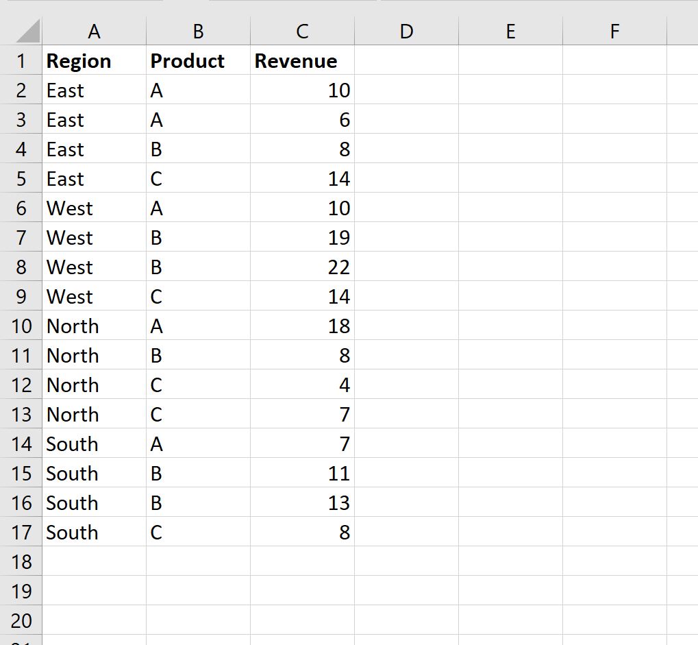
Suppose we have the following dataset that shows the total sales of certain products in certain regions for a company:

Now suppose we’d like to filter for rows where the Region does not contain “East.”
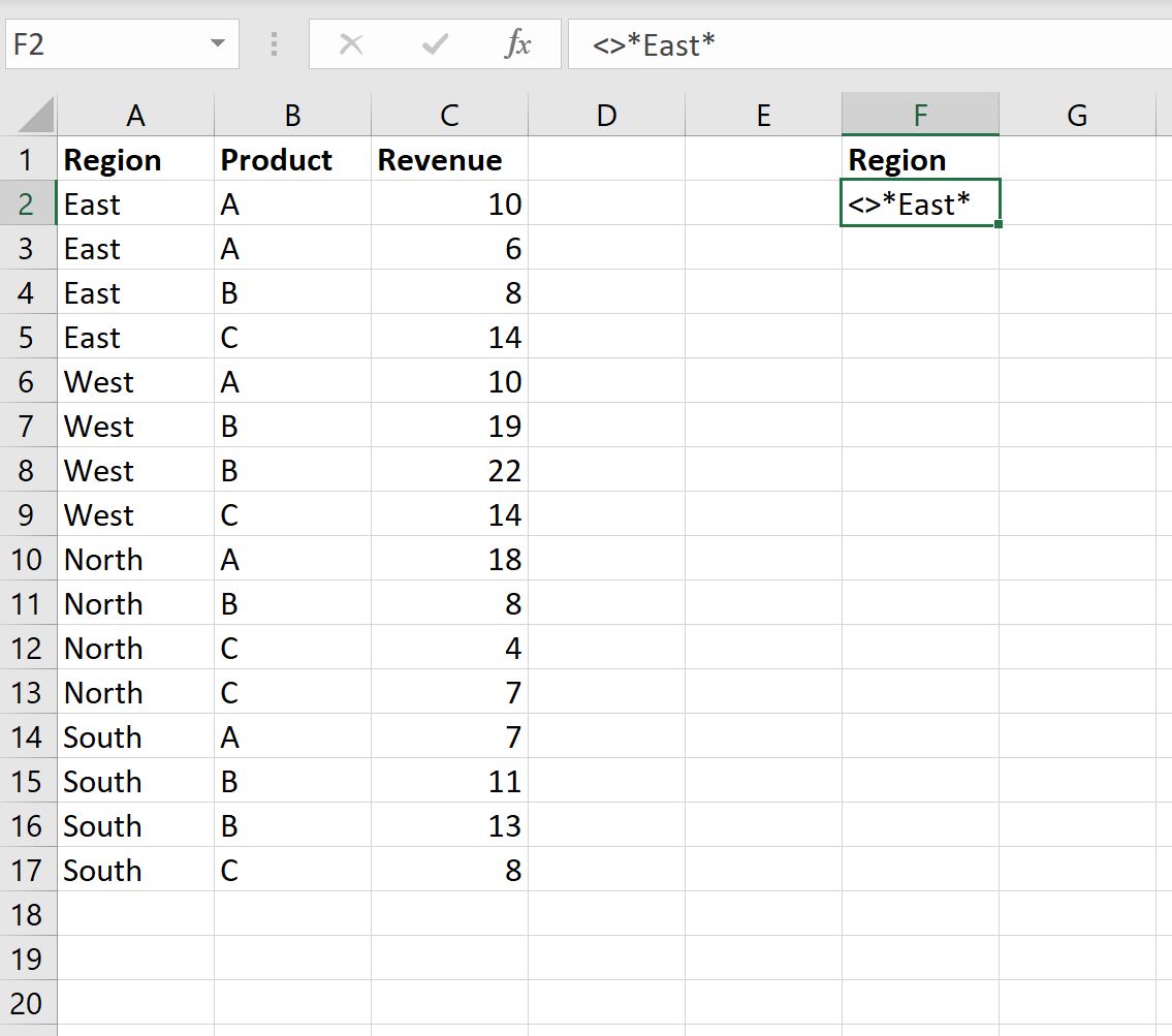
To do so, we can define a criteria range:

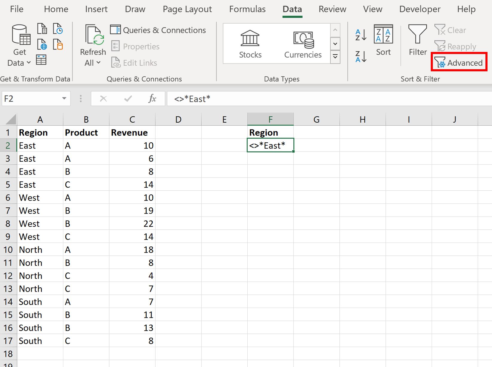
Next, we can click the Data tab and then click the Advanced Filter button:

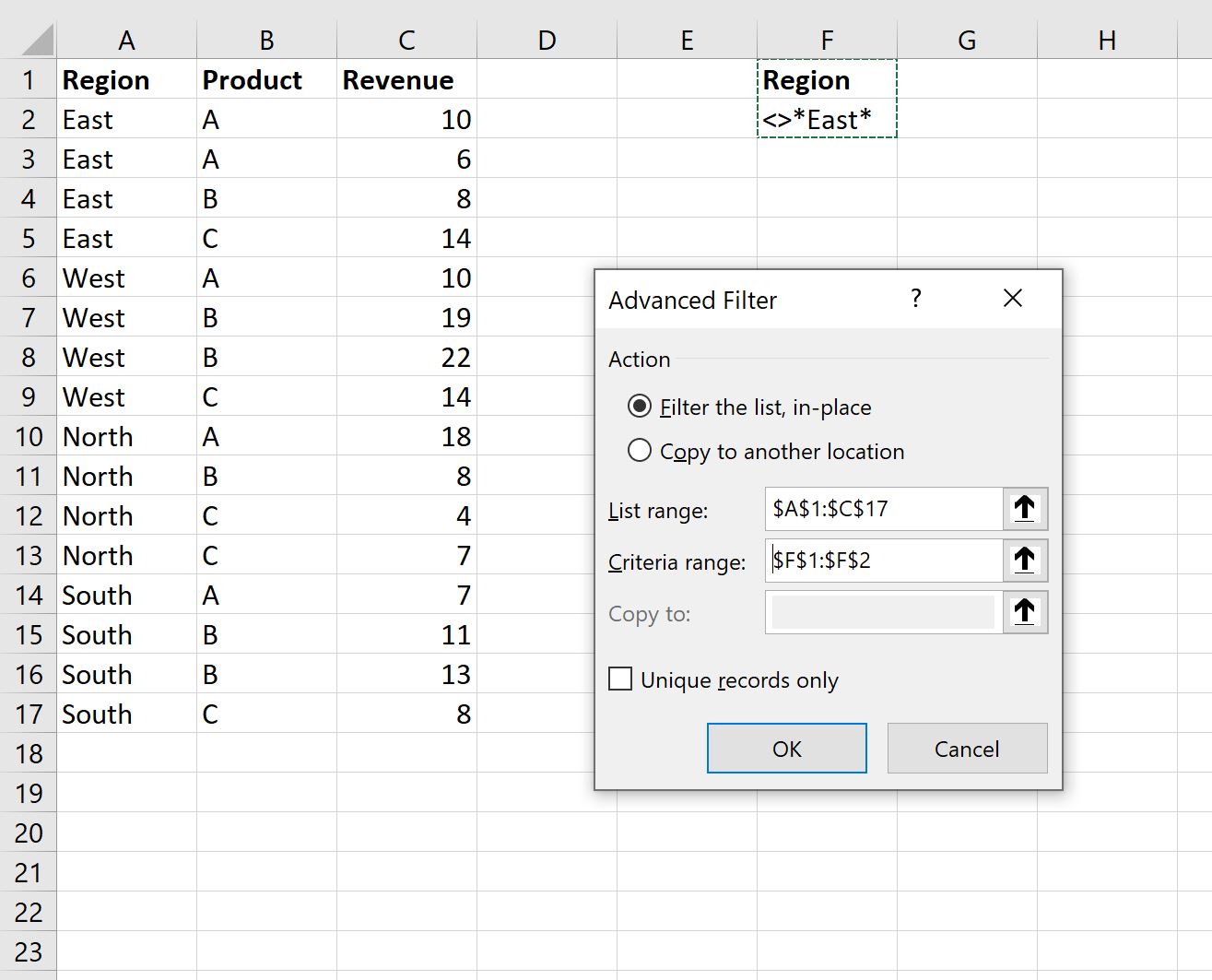
We’ll choose A1:C17 as the list range and F1:F2 as the criteria range:

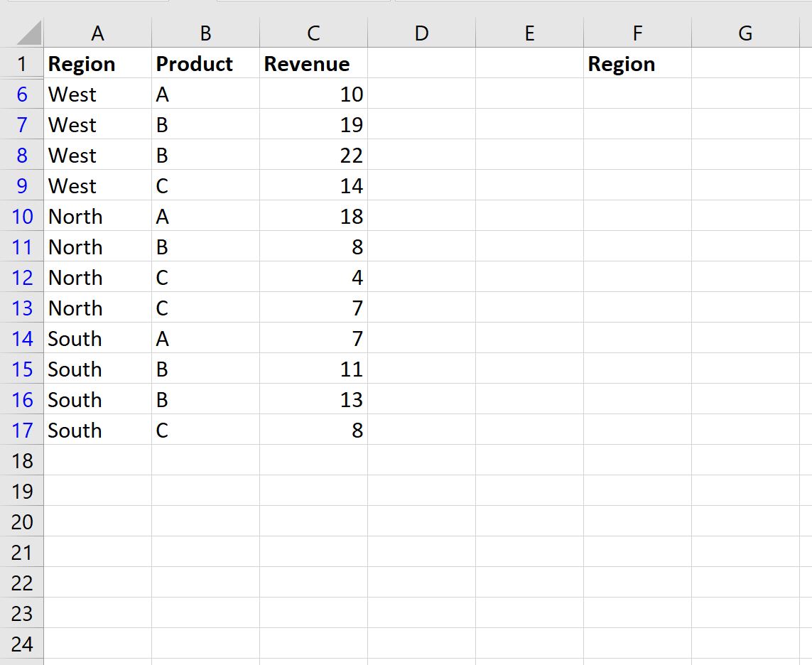
Once we click OK, the dataset will be filtered to only show rows where the Region does not contain “East“:

Example 2: Filter for Rows that Do Not Contain One of Multiple Text
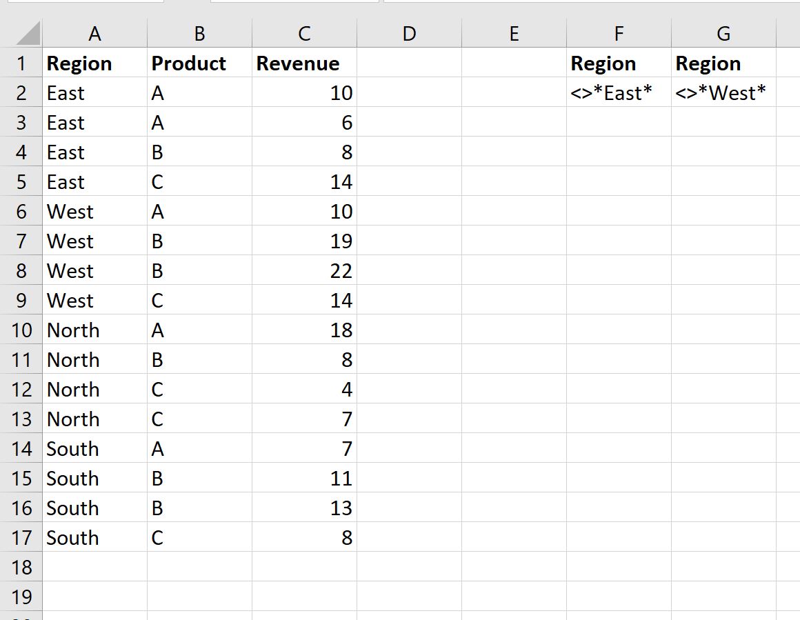
Suppose we have the following dataset that shows the total sales of certain products in certain regions for a company:
Now suppose we’d like to filter for rows where the Region does not contain “East” or “West.”
To do so, we can define a criteria range:

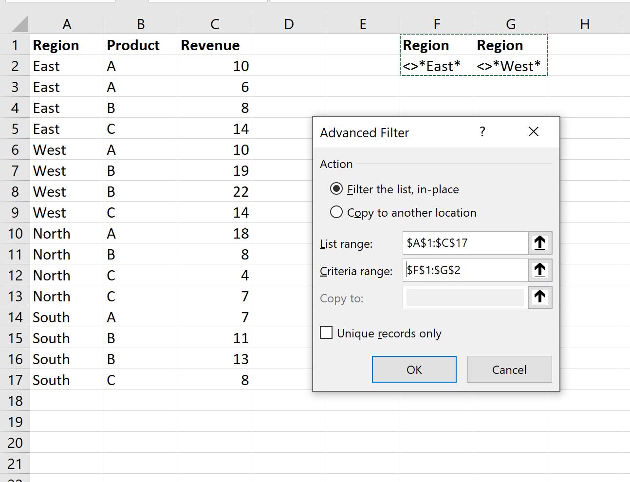
Next, we can click the Data tab and then click the Advanced Filter button.
We’ll choose A1:C17 as the list range and F1:G2 as the criteria range:

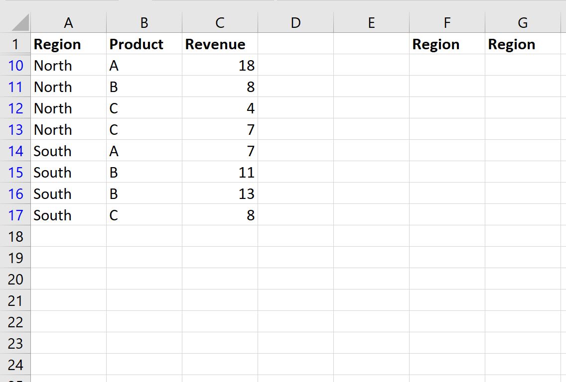
Once we click OK, the dataset will be filtered to only show rows where the Region does not contain “East” or “West“:

Additional Resources
The following tutorials explain how to perform other common operations in Excel:
How to Filter Multiple Columns in Excel
How to Sum Filtered Rows in Excel
How to Delete Filtered Rows in Excel
In this example, the goal is to count cells that do not contain a specific substring. This problem can be solved with the COUNTIF function or the SUMPRODUCT function. Both approaches are explained below. Although COUNTIF is not case-sensitive, the SUMPRODUCT version of the formula can be adapted to perform a case-sensitive count. For convenience, data is the named range B5:B15.
COUNTIF function
The COUNTIF function counts cells in a range that meet supplied criteria. For example, to count the number of cells in a range that contain «apple» you can use COUNTIF like this:
=COUNTIF(range,"apple") // equal to "apple"
Note this is an exact match. To be included in the count, a cell must contain «apple» and only «apple». If a cell contains any other characters, it will not be counted. To reverse this operation and count cells that do not contain «apple», you can add the not equal to (<>) operator like this:
=COUNTIF(range,"<>apple") // not equal to "apple"
The goal in this example is to count cells that do not contain specific text, where the text is a substring that can be anywhere in the cell. To do this, we need to use the asterisk (*) character as a wildcard. To count cells that contain the substring «apple», we can use a formula like this:
=COUNTIF(range,"*apple*") // contains "apple"
The asterisk (*) wildcard matches zero or more characters of any kind, so this formula will count cells that contain «apple» anywhere in the cell. To count cells that do not contain the substring «apple», we add the not equal to (<>) operator like this:
=COUNTIF(range,"<>*apple*") // does not contain "apple"
The formulas used in the worksheet shown follow the same pattern:
=COUNTIF(data,"<>*a*") // does not contain "a"
=COUNTIF(data,"<>*0*") // does not contain "0"
=COUNTIF(data,"<>*-r*") // does not contain "-r"
Data is the named range B5:B15. The COUNTIF function supports three different wildcards, see this page for more details.
Note the COUNTIF formula above won’t work if you are targeting a particular number and cells contain numeric data. This is because the wildcard automatically causes COUNTIF to look for text only (i.e. to look for «2» instead of just 2). In addition, COUNTIF is not case-sensitive, so you can’t perform a case-sensitive count. The SUMPRODUCT alternative explained below can handle both situations.
With a cell reference
You can easily adjust this formula to use a cell reference in criteria. For example, if A1 contains the substring you want to exclude from the count, you can use a formula like this:
=COUNTIF(range,"<>*"&A1&"*")
Inside COUNTIF, the two asterisks and the not equal to operator (<>) are concatenated to the value in A1, and the formula works as before.
Exclude blanks
To exclude blank cells, you can switch to COUNTIFS function and add another condition like this:
=COUNTIFS(range,"<>*a*",range,"?*") // requires some text
The second condition means «at least one character».
See also: 50 examples of formula criteria
SUMPRODUCT function
Another way to solve this problem is with the SUMPRODUCT function and Boolean algebra. This approach has the benefit of being case-sensitive if needed. In addition, you can use this technique to target a number inside of a number, something you can’t do with COUNTIF.
To count cells that contain specific text with SUMPRODUCT, you can use the SEARCH function. SEARCH returns the position of text in a text string as a number. For example, the formula below returns 6 since the «a» appears first as the sixth character in the string:
=SEARCH( "a","The cat sat") // returns 6
If the text is not found, SEARCH returns a #VALUE! error:
=SEARCH( "x","The cat sat") // returns #VALUE!
Notice we do not need to use any wildcards because SEARCH will automatically find substrings. If we get a number from SEARCH, we know the substring was found. If we get an error, we know the substring was not found. This means we can add the ISNUMBER function to evaluate the result from SEARCH like this:
=ISNUMBER(SEARCH( "a","The cat sat")) // returns TRUE
=ISNUMBER(SEARCH( "x","The cat sat")) // returns FALSE
To reverse the operation, we add the NOT function:
=NOT(ISNUMBER(SEARCH( "a","The cat sat"))) // FALSE
=NOT(ISNUMBER(SEARCH( "x","The cat sat"))) // TRUE
We now have what we need to count cells that do not contain a substring with SUMPRODUCT. Back in the example worksheet, to count cells that do not contain «a» with SUMPRODUCT, you can use a formula like this
=SUMPRODUCT(--NOT(ISNUMBER(SEARCH("a",data))))
Working from the inside out, SEARCH is configured to look for «a»:
SEARCH("a",data)
Because data (B5:B15) contains 11 cells, the result from SEARCH is an array with 11 results:
{1;1;1;1;2;2;#VALUE!;#VALUE!;#VALUE!;#VALUE!;#VALUE!}
In this array, numbers indicate the position of «a» in cells where «a» is found. The #VALUE! errors indicate cells where «a» was not found. To convert these results into a simple array of TRUE and FALSE values, we use the ISNUMBER function:
ISNUMBER(SEARCH("a",data))
ISNUMBER returns TRUE for any number and FALSE for errors. SEARCH delivers the array of results to ISNUMBER, and ISNUMBER converts the results to an array that contains only TRUE and FALSE values:
{TRUE;TRUE;TRUE;TRUE;TRUE;TRUE;FALSE;FALSE;FALSE;FALSE;FALSE}
In this array, TRUE corresponds to cells that contain «a» and FALSE corresponds to cells that do not contain «a». This is exactly the opposite of what we need, so we use the NOT function to reverse the array:
NOT(ISNUMBER(SEARCH("a",data)))
The result from the NOT function is:
{FALSE;FALSE;FALSE;FALSE;FALSE;FALSE;TRUE;TRUE;TRUE;TRUE;TRUE}
In this array, the TRUE values represent cells we want to count. However, we first need to convert the TRUE and FALSE values to their numeric equivalents, 1 and 0. To do this, we use a double negative (—):
--NOT(ISNUMBER(SEARCH("a",data)))
The result inside of SUMPRODUCT looks like this:
=SUMPRODUCT({0;0;0;0;0;0;1;1;1;1;1}) // returns 5
With a single array to process, SUMPRODUCT sums the array and returns 5 as a final result.
One benefit of this formula is it will find a number inside a numeric value. In addition, there is no need to use wildcards to indicate position, because SEARCH will automatically look through all text in a cell.
Case-sensitive option
For a case-sensitive count, you can replace the SEARCH function with the FIND function like this:
=SUMPRODUCT(--NOT(ISNUMBER(FIND("A",data))))
The FIND function works just like the SEARCH function, but is case-sensitive. Notice we have replaced «a» with «A» because FIND is case-sensitive. If we used «a», the result would be 11 since there are no cells in B5:B15 that contain a lowercase «a». This example provides more detail.
Note: the SUMPRODUCT formulas above are more complex, but using Boolean operations in array formulas is a more powerful and flexible approach. It is also an important skill in modern functions like FILTER and XLOOKUP, which often use this technique to select the right data. The syntax used by COUNTIF is unique to a group of eight functions and is therefore not as useful or portable.
EXPLANATION
This tutorial shows how to test if a range does not contain a specific value and return a specified value if the formula tests true or false, by using an Excel formula and VBA.
This tutorial provides one Excel method that can be applied to test if a range does not contain a specific value and return a specified value by using an Excel IF and COUNTIF functions. In this example, if the Excel COUNTIF function returns a value of 0, meaning the range does not have cells with a value of 505, the test is TRUE and the formula will return a «Not in Range» value. Alternatively, if the Excel COUNTIF function returns a value of greater than 0, meaning the range has cells with a value of 505, the test is FALSE and the formula will return a «In Range» value.
This tutorial provides one VBA method that can be applied to test if a range does not contain a specific value and return a specified value and return a specified value.
FORMULA
=IF(COUNTIF(range, value)=0, value_if_true, value_if_false)
ARGUMENTS
range: The range of cells you want to count from.
value: he value that is used to determine which of the cells should be counted, from a specified range, if the cells’ value is equal to this value.
value_if_true: Value to be returned if the range does not contains the specific value.
value_if_false: Value to be returned if the range contains the specific value.
17 авг. 2022 г.
читать 2 мин
Вы можете использовать следующий синтаксис для фильтрации строк, которые не содержат определенного текста в расширенном фильтре Excel:
<>*sometext*
В следующих примерах показано, как использовать эту функцию в двух разных сценариях:
- Фильтр для строк, которые не содержат один конкретный текст
- Отфильтровать строки, которые не содержат ни одного из нескольких текстов
Пример 1. Фильтрация строк, не содержащих одного определенного текста
Предположим, у нас есть следующий набор данных, который показывает общий объем продаж определенных продуктов в определенных регионах для компании:
Теперь предположим, что мы хотим отфильтровать строки, в которых регион не содержит « Восток ».
Для этого мы можем определить диапазон критериев:
Затем мы можем щелкнуть вкладку « Данные », а затем нажать кнопку « Расширенный фильтр »:
Мы выберем A1:C17 в качестве диапазона списка и F1:F2 в качестве диапазона критериев :
Как только мы нажмем OK , набор данных будет отфильтрован, чтобы отображались только строки, в которых регион не содержит « Восток »:
Пример 2. Фильтрация строк , не содержащих ни одного из нескольких текстов
Предположим, у нас есть следующий набор данных, который показывает общий объем продаж определенных продуктов в определенных регионах для компании:
Теперь предположим, что мы хотим отфильтровать строки, в которых регион не содержит « Восток » или « Запад ».
Для этого мы можем определить диапазон критериев:
Затем мы можем щелкнуть вкладку « Данные », а затем нажать кнопку « Расширенный фильтр ».
Мы выберем A1: C17 в качестве диапазона списка и F1: G2 в качестве диапазона критериев :
Как только мы нажмем « ОК », набор данных будет отфильтрован, чтобы отображать только те строки, в которых «Регион» не содержит « Восток » или « Запад »:
Дополнительные ресурсы
В следующих руководствах объясняется, как выполнять другие распространенные операции в Excel:
Как отфильтровать несколько столбцов в Excel
Как суммировать отфильтрованные строки в Excel
Как удалить отфильтрованные строки в Excel
At present, we can’t use wildcards in the new Filter function in Excel 365.
It doesn’t support the wildcards asterisk, tilde, and question mark.
* – Asterisk~ – Tilde? – Question Mark
But that doesn’t mean we can’t apply partial match filtering in Excel 365 using the Filter function.
We can use two functions as alternatives to wildcards in the Filter function in Excel 365.
Before going to the said two Excel functions, first, let’s start with the purpose of such kind of filtering.
Partial matches are the purpose of using wildcards in the Filter function in Excel 365.
For example, we have a column in an Excel spreadsheet with some product IDs.
I mean the IDs starting with the letter “A” for “Apple,” “M” for “Mango,” and so on.
Suppose, for “Apple” based on the grade, the IDs are defined as “A1,” “A2,” “A3,” and “A4” (which may not be so in real-life).
How to Filter all the IDs related to “Apple?”
| IDs | Stock (MT) |
| A1 | 1 |
| A2 | 1 |
| A1 | 1 |
| A2 | 2 |
| A2 | 2 |
| M1 | 2 |
| M1 | 2 |
| M2 | 2 |
| M2 | 1 |
Here we can use either of the Excel functions Search or Find within the Filter function as an alternative to the asterisk wildcard character.
Two Wildcard Alternatives in Filter Function in Excel 365
As I have mentioned above, the alternatives are the Search and Find functions.
Here are two examples of the usage.
Open an Excel spreadsheet and copy-paste the above table (range A1:B10).
Let’s use the standard Excel Filter formula here to filter all the rows related to the fruit “Apple” (IDs starting with “A”).
=FILTER(A2:B10,A2:A10="A")You would get an #CALC! error as there are no matches (empty array).
If you hover your mouse pointer over the error cell (the cell containing the error in Excel), you can see the tooltip explanation.
Empty arrays are not supported
What is the solution?
Search – Case Insensitive Wildcard Alternative in Filter Function in Excel 365
Here is the solution using the Search function within the Filter function in Excel.
=FILTER(A2:B10,ISNUMBER(SEARCH("A",A2:A10)))
This way, we can use wildcards in Filter Function in Excel 365.
Excel Formula Explanation
The ISNUMBER and SEARCH Combination is the key in the above Excel Formula.
The Search formula returns an array with some values (numbers) and errors.

The cells containing numbers are the rows that match the character (filter condition) “A” in A2:A10 and the cells containing #VALUE! are the rows that do not match the condition.
Wrap the above Excel formula with Isnumber to return TRUE for the cells containing numbers and FALSE for errors.
=ISNUMBER(SEARCH("A",A2:A10))
The Excel Filter filters the rows containing TRUE values.
The above is an alternative to wildcards use in the Filter function in Excel 365.
Please note that the Excel Search function is case insensitive and no doubt the above filter formula too.
Find – Case Sensitive Wildcard Alternative in Filter Function in Excel 365
The above Excel formula is case insensitive and so won’t differentiate capital and small case letters.
For case-sensitive Filter formula with wildcard use, replace the Search function in the above formula with the Find function.
No other change is required!
=FILTER(A2:B10,ISNUMBER(FIND("A",A2:A10)))
Contain and Does Not Contain in Excel Filter Formula
Before winding up this Excel tutorial, here are two more examples.
This time, let’s see how to filter a list that contains a specific word and doesn’t contain a specific word.
Example:

Contain
Assume column A in Excel contains a list of names (see the above image).
In that, I want to filter the names that contain the first or second name “Martin.”
We can use either of the above two Excel formulas (Filter using ISNUMBER + FIND or Filter using ISNUMBER + SEARCH).
Here I am going to use the FIND.
Here is the formula in cell C2 as per the image above.
=FILTER(A2:A8,ISNUMBER(FIND("Martin",A2:A8)))It will filter all the names that contain the first or second name “Martin.”
Doesn’t Contain
By simply adding =FALSE that just before the final closing bracket, we can make the above Excel formula to doesn’t contain (opposite Filter).
Here is the formula in cell E2 as per the image above.
=FILTER(A2:A8,ISNUMBER(FIND("Martin",A2:A8))=FALSE)I hope you found this Excel tutorial helpful!
Excel 365 Filter Resources:
- AND, OR Use in Filter Function in Excel 365 – Formula Examples.
- How to Get Title Row with Filter Formula Result in Excel.
- Not Equal to in Filter Function in Excel.
- Filter Nth Occurrence in Excel 365 (Formula Approach).
- How to Use a Dynamic List as Criteria in Filter Function in Excel 365.
-
11-08-2012, 05:01 PM
#1

Registered User
excel advanced filter does not contain text
I am trying to do an advanced filter by doing a does not contain «xxx». Here is a simplified example.
Service Requested
Service Performed
seal
test1
frost
test2
test3
seal
test4
frost
board6
test5
test6
board1
test7
test8
seal
board2
frost
board3
board4
seal
board5
frost
I would to filter both Service Requested & Service Performed by the cells that contain either seal or frost in either column, but do not contain board. This is the table for the advanced filter that I have been using with no luck:
Service Requested
Service Performed
Service Requested
Service Performed
*seal*
<>*Board*
*frost*
<>*Board*
*seal*
<>*Board*
*frost*
<>*Board*
The end result would look like this:
Service Requested
Service Performed
seal
test1
frost
test2
test3
seal
test4
frost
How do I use the does not contain «text» in the advanced filter?
Last edited by refrigman; 11-09-2012 at 10:11 AM.
-
11-08-2012, 10:22 PM
#2
Re: excel advanced filter does not contain text
Hi
Raw data in range A1:B12
Criteria in range E1:F5
Criteria Data
E1: Requested
E2: =»*seal*»
E3: =»*frost*»
E4: =»<>»&»*board*»
E5: =»<>»&»*board*»
F1: Service Performed
F2: =»<>»&»*board*»
F3: =»<>»&»*board*»
F4: =»*seal*»
F5: =»*frost*»Copy to Range J1:K1 (which have the appropriate headings)
See how that goes.
rylo
-
11-08-2012, 11:10 PM
#3
Re: excel advanced filter does not contain text
if you’re data is in columns A and B, use a helper column in C and copy this down…
=IF(OR(NOT(ISERROR(SEARCH(«board»,A2,1))),NOT(ISERROR(SEARCH(«board»,B2,1)))),»»,
IF(OR(A2=»seal»,A2=»frost»,B2=»seal»,B2=»frost»),1,»»))
filter on C1. Use code tags for VBA. [code] Your Code [/code] (or use the # button)
2. If your question is resolved, mark it SOLVED using the thread tools
3. Click on the star if you think someone helped youRegards
Ford
-
11-09-2012, 10:11 AM
#4
Registered User
Re: excel advanced filter does not contain text
Looks like you are both right. Thanks for the help.

