
You can control the display of formulas in the following ways:
Click on Formulas and then click on Show Formulas to switch between displaying formulas and results.
Press CTRL + ` (grave accent).
Note: This procedure also prevents the cells that contain the formula from being edited.
-
Select the range of cells whose formulas you want to hide. You can also select nonadjacent ranges or the entire sheet.
-
Click Home > Format > Format Cells.
-
On the Protection tab, select the Hidden check box.
-
Click OK.
-
Click Review > Protect Sheet.
-
Make sure the Protect worksheet and contents of locked cells check box is selected, and then click OK.
Click the Review tab, and then click Unprotect Sheet. If the Unprotect Sheet button is unavailable, turn off the Shared Workbook feature first.
If you don’t want the formulas hidden when the sheet is protected in the future, right-click the cells, and click Format Cells. On the Protection tab, clear the Hidden check box.
Click on Formulas and then click on Show Formulas to switch between displaying formulas and results.
As soon as you type a formula in Excel and hit enter, it would return the calculated result, and the formula would disappear.
That’s how it’s supposed to work.
But what if you want to show formulas in the cells and not the calculated values.
In this Excel tutorial, I will cover the following topics:
- How to Show Formulas in Excel instead of the values.
- How to Print the formulas in Excel.
- How to Show Formulas in Excel in Selected Cells Only.
- What to Do when Excel Shows Formulas Instead of the Calculated Values.
Show Formulas in Excel Instead of the Values
Here are the steps to show formulas in Excel instead of the value:
As soon as you click on Show Formulas, it will make the formulas in the worksheet visible. It’s a toggle button, so you can click on it again to make the formulas be replaced by its calculated result.
It’s a toggle button, so you can click on it again to make the formulas be replaced by its calculated result.
As shown below, column I has the formulas. As soon as ‘Show Formulas’ button is clicked, the cells show the formulas instead of the value.
You can also use the Excel keyboard shortcut – Control + ` (you will find this key in the top-left part of the keyboard, under the Escape key).
Note: This is a sheet level technique. This means that when you use the Show Formulas option or the shortcut, it will only show the formulas in the active sheet. All the other worksheets will be unaffected. To show formulas in other worksheets, you will have to go to that sheet and use this shortcut (or ribbon button).
In some cases, you may have a lot of worksheets and you want to show the formulas in all the worksheets in the workbook.
Here are the steps that will show the formulas in all the worksheets in Excel:
As mentioned, while this may seem to have more steps as compared to a shortcut or the ‘Show Formulas’ button in the ribbon, it’s useful when you have multiple worksheets and you want to show the formulas in all these worksheets.
How to Print Formulas in Excel
Here are the steps to print formulas in Excel:
- Go to Formula tab.
- Click on the Show Formula option.
- Go to File –> Print.
The above steps would ensure that it prints the formulas and not the values.
Show Formulas in Excel Instead of the Value in Selected Cells Only
The above methods covered so far would show all the formulas in a worksheet.
However, you may want to show the formulas in some selected cells only.
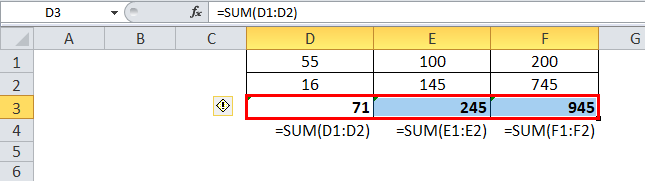
For example, as an Excel trainer, I often create templates where I show the formula in one cell and its result in another cell (as shown below).
Here are the steps to show formulas in Excel in selected cells only:
This will show formulas in all the selected cell while the remaining cells would remain unchanged.
Note: Entering a space before the formula makes it a text string and the space character is visible before the equal to sign. On the other hand, using an apostrophe before the equal to sign make the formula a text string, however, the apostrophe isn’t visible in the cell (it shows up only in the formula bar and in the edit mode).
How to Handle Excel Showing Formulas Instead of Calculated Values
Sometimes, you may find that the cells in Excel are showing the formula instead of the value.
There are a couple of reasons why this may happen:
- The ‘Show Formulas’ mode is enabled or you may have accidently hit the Control + ` shortcut. To disable it, simply use the shortcut again or click on the ‘Show Formula’ option in the Formulas tab.
- It could be due to the presence of a space character or apostrophe before the equal to sign in the formula. The presence of these before the equal to sign makes the cell format as text and the formula shows up instead of the value. To handle this, simply remove these. You can use find and replace to do this.
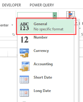
- If a cell has ‘Text’ formatting applied to it and you enter the formula and hit enter, it will continue to show the formula instead of the calculated value. To fix this issue, go to the Home tab and with the Number group, change the formatting to General.

You May Also Like the Following Excel Tutorials:
- How to Convert Formulas to Values in Excel.
- How to Multiply in Excel Using Paste Special.
- How to Lock Formulas in Excel.
- Absolute, Relative, and Mixed Cell References in Excel.
- Hide Zero Values in Excel (Make Cells Blank If the Value is 0)
How to Show Formulas in Excel: 4 easy methods (2023)
Have you ever worked on a spreadsheet densely packed with formulas?
In such a case, to make sense of how each of the formulas works and how the results are derived, you might want to see the formulas in the cells.
This guide will teach you how to display formulas in Excel. 😀
Download our sample workbook here to follow the guide as we dive into the details of this topic.
How to show formulas in Excel from ribbon
Type any formula into Excel, say = 2+ 2, and hit ‘Enter’.

It’ll take Excel less than a nano-second to run the formula above and display results.
But what if you want the formula ‘= 2 + 2’ to be on the display only? Here’s how you can do it.
1. Select any cell of your worksheet.
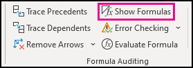
2. Go to the Ribbon > Formulas Tab > Formula Auditing group.

3. Click on the button ‘Show Formulas’.
4. Excel will now display the formulas for all cells in the worksheet and not the result.

Nice! How can we now get back the results?
5. Go back to the Ribbon > Formulas Tab > Formula Auditing group.
6. Again Click on the button ‘Show Formulas’, and there you go.

Excel again displays the result and not the formula.
Show formulas using the shortcut command
You can also display formulas in Excel by using a shortcut key. It is swift and easy.
1. Click any cell of an Excel worksheet.
2. Press the Ctrl key + Grave Accent Key ( ` ).
Can’t find the grave accent key on your keyboard? Look to the left of 1 from the number keys.

This puts all cells of that worksheet to display formulas instead of the results.

Note that this shortcut only displays formulas for all cells of the active worksheet. Not the entire workbook.
4. Want to go back already? Press the Ctrl key + Grave Accent Key ( ` ) again.
Excel takes the display back to the results. No more formulas.

That’s for Windows users. Does the method change for Mac users?
Certainly not. Even if you’re a Mac user, the process remains the same. Press the Control key + grave accent key (`) to display formulas.
Whenever you’re done and want to go back to the default display, again press the same keys together.
How to display formulas in specific cells only
We’ve come across two methods to display formulas in Excel already. However, did you notice something?
Both the above methods would display formulas for all the cells of the active worksheet.
But what if you only want to display the formula of a selected cell? There are two ways you can achieve this.
i. Add a space before the formula
Take the following image as an example, where cells A1, A2, and A3 have a formula.

You want to display the formula for cells A1 and A2 only and not for cell A3.
1. Select Cell A1 and A2.
2. Go to Home Tab > Editing group > Find & Select > Replace.

This launches the Find and Replace dialog box as below.

You may use the keyboard shortcut Control + H to launch the Find & Replace feature.
3. Against the Find tab, punch in an equal sign ‘=’.
4. Against the Replace tab, punch in an equal sign but after a space character ‘ =’.

This way the formulas in the selected cells will not start with an equal sign but a space character. And Excel only recognizes a formula when it starts with an equal sign.
5. The results only in the selected cells will be replaced by formulas as follows.

The selected range (Cell A1 and A2) shows formulas. Cell A3 continues to show the results.
ii. Add an apostrophe before the formula
If you do not want a space character visible in the cell, you may use this method instead.
1. Select Cell A1 and A2.
2. Go to Home Tab > Editing group > Find & Select > Replace.
3. In the Find and Replace dialog box, punch in an equal sign (=) against Find.
4. Against the Replace tab, punch in an equal sign but after an apostrophe (‘=).

This way the formulas in the selected cells will not start with an equal sign but an apostrophe. Whenever something starts with an apostrophe in a cell, Excel takes it as a text string.
5. The results only in the selected cells will be replaced by formulas as follows.

However, unlike the space character, the apostrophe is not visible in the cell. It is only visible in the formula bar or in the edit mode.
Pro Tip!
If you are in a hurry and only want to have a glimpse of the formula in a cell, the above methods might not suit you.
To check the formula to a cell, you may press ‘F2’. This will instantly show the formula running behind a cell.
However, as soon as you click away or press enter, the formula would be replaced by the result.
How to show formulas with the FORMULATEXT function
It’s time we introduce you to a modern-day Excel function. We bet you’ve not heard of it before.
The image below has a cell that contains a formula.

Do you want this formula to appear as it appears in the formula bar but in a different cell?
1. Activate a cell and write the FORMULATEXT function as follows.
= FORMULATEXT (A1)
Write that as the 2nd argument in the MATCH function, replacing what’s currently there.

The FORMULATEXT function of Excel has a single argument – the reference argument.
In the reference argument, you create a reference to the cell whose formula you want to be displayed. We have created the reference to cell A1.
2. Hit enter to see the results as follows.

Note how Excel displays the formula of the referenced cell.
You can display the formula of any cell doing so. 😉
Pro Tip!
What if cell A1 above contained a formula with reference to another workbook?
The FORMULATEXT function would give back a #N/A error if that workbook is not open in the background.
How to select all formulas in the selection
If you’ve only received an Excel file prepared by someone else, how can you quickly identify the cells that have a formula running behind them?
The image below has a list of numbers (some of which are the result of a formula). Whereas, some others are simply punched in numeric values.

To select the formulas for the first six cells of this list (A1 to A6), follow these steps.
1. Select the cells (Cell A1 to A6).
2. Go to the Home Tab > Editing > Find & Select > Go to Special.

Or press down the Control key + G.
3. From the ‘Go To’ dialog box, click special.

4. Check ‘Formulas’ and press okay.

5. Excel selects all the cells that have a formula from Cell A1 to A6.

A5 and A6 do not have any formulas but only numbers. Hence, Excel did not select them.
You can format cells (highlight them) or check the count of these cells from the status bar.

How to print formulas
Whenever you print an Excel sheet, the print contains the calculated results. Not the formulas.
Need the print of your spreadsheet to have the formulas instead of the results?
1. Perform either of the methods above to display the formula in cells.
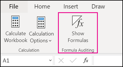
2. Once your worksheet begins displaying formulas, go to File Tab > Print..

Or just use the print keyboard shortcut. Hit the Control key + P.
3. Here’s what the print preview looks like.

The final printed version would contain formulas and not their calculated results.
That’s it – Now what?
The tutorial above guides you on everything about formulas. Starting from displaying formulas in Excel to printing them.
Once you have a good grip on how formulas work in your spreadsheet, everything will begin to make better sense.
But, do you know how to use some of the most crucial formulas/functions of Excel? Like the VLOOKUP, SUMIF, and the IF functions?
Here’s my 30-minutes free email course that will help you master these and many more functions of Excel in no time.
Kasper Langmann2023-01-19T12:21:09+00:00
Page load link
How to Hide Formulas in Excel?
Hiding formulas in Excel is a method when we do not want them to be displayed in the formula bar when we click on a cell with formulas. We can format the cells, check the hidden checkbox, and then protect the worksheet. It will prevent the formula from displaying in the “Formula” tab. Only the result of the formula will be visible.
Table of contents
- How to Hide Formulas in Excel?
- 13 Easy Steps to Hide Formula in Excel (with Example)
- Things to Remember
- Recommended Articles
13 Easy Steps to Hide Formula in Excel (with Example)
Let us understand the steps to hide formulas in Excel with examples.
You can download this Hide Formula Excel Template here – Hide Formula Excel Template
Step 1:
Following are the 13 steps that we can use to hide formulas in Excel:
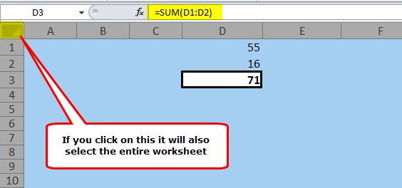
- First, we must select the entire worksheet by pressing the shortcut key “Ctrl + A.”

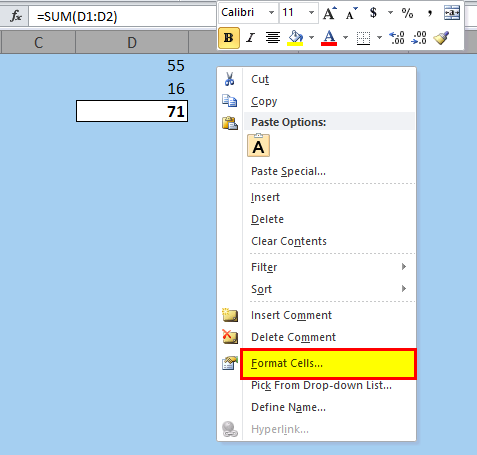
- Now, on any cell, right-click and select “Format Cells” or press “Ctrl + 1.”

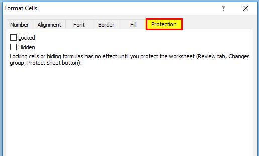
- Once the above option is selected, it may open the below dialog box and select “Protection.”

- Once the “Protection” tab is selected, uncheck the “Locked” option.
As a result, this will unlock all the cells in the worksheet. Remember, this may unlock the cells in the active worksheet in all the remaining worksheets. It remains locked only.
- If we observe as soon as we unlock the cells, Excel will notify us of an error as “Unprotected Formula.”

- Select only the formula cells and lock them. For example, we have three formulas in the worksheet, and we selected all three.

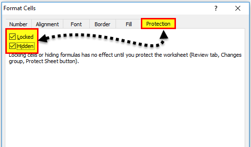
- Now, we must open the “Format Cells, select the “Protection” tab, and check the “Locked” and “Hidden” options.

Note: If we have many formulas in the Excel worksheet, we want to select each one of them, then we need to follow the below steps.
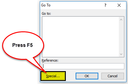
- Now, press the F5 (shortcut key to “Go to Special”) and select “Special.”

- Consequently, this will open up the below dialog box. Select “Formulas” and click “OK.” It would select all the formula cells in the worksheet.

Now, it has selected all the formula cells in the entire worksheet.
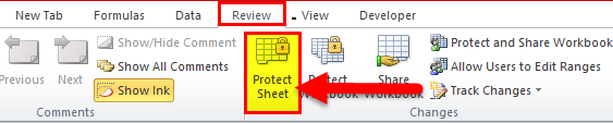
- Protect the sheet once the formula cells are selected, locked, and hidden. Then, go to the “Review” tab and “Protect Sheet.”

- Click on the “Protect Sheet” in Excel, and the dialog box may open up. Select only “Select locked cells” and “Select unlocked cells.” Type the password carefully because we cannot edit those cells if we forget the password.

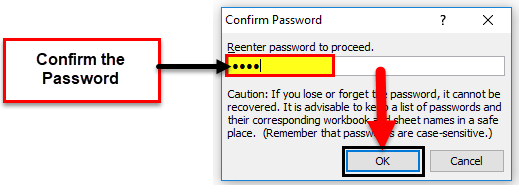
- Click on the “OK” button. It will again ask us to confirm the password. Enter the same password again.

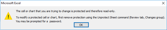
- Click on the “OK.” Now, our Excel formulas are locked and protected with a password. Suppose we cannot edit the password without the password. Then, if we try editing the formula, Excel will show the below warning message for us. Also, the formula bar does not show anything.


Things to Remember
- The most common way of hiding the formulas is by locking the particular cell and password protecting the worksheet.
- The first basic thing we need to do is “unlock all the cells in the active worksheet.” You must be wondering why we need to unlock all the cells in the worksheet where we did not even start the process of locking the cells in the worksheet.
- We need to unlock first by default. Then, Excel turns on excel Locked cellIn Excel, cells are locked to protect them from unwanted editing, deleting, and overwriting. Locking cells is specifically beneficial in cases where an excel worksheet needs to be shared with several colleagues.read more. However, we can still edit and manipulate the cells because we have not yet password-protected the sheet.
- We can open the “Go to Special” dialog box by pressing the “F5” shortcut.
- We must use the “Ctrl + 1” as the shortcut key to open the formatting options.
- Remember the password carefully. Otherwise, we cannot unprotect the worksheet.
- Only the password known person can edit the formulas.
Recommended Articles
This article has been a guide to Hide Formula in Excel. Here, we discuss how to hide formulas in Excel using the “Protection” tab to lock the cell and practical examples. You may learn more about Excel from the following articles: –
- Shortcut to Hide in Excel
- Unhide Sheets in Excel
- VBA Hide Columns
- How to Unhide Columns in Excel?
Содержание
- Пропажа строки формул
- Причина 1: изменение настроек на ленте
- Причина 2: настройки параметров Excel
- Причина 3: повреждение программы
- Вопросы и ответы

Строка формул – один из основных элементов приложения Excel. С её помощью можно производить расчеты и редактировать содержимое ячеек. Кроме того, при выделении ячейки, где видно только значение, в строке формул будет отображаться расчет, с помощью которого это значение было получено. Но иногда данный элемент интерфейса Экселя пропадает. Давайте разберемся, почему так происходит, и что в этой ситуации делать.
Пропажа строки формул
Собственно, пропасть строка формул может всего по двум основным причинам: изменение настроек приложения и сбой в работе программы. В то же время, эти причины подразделяются на более конкретные случаи.
Причина 1: изменение настроек на ленте
В большинстве случаев исчезновение строки формул связано с тем, что пользователь по неосторожности снял галочку, отвечающую за её работу, на ленте. Выясним, как исправить ситуацию.
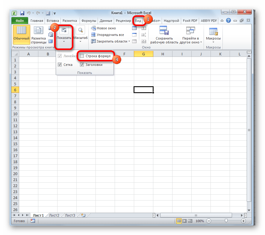
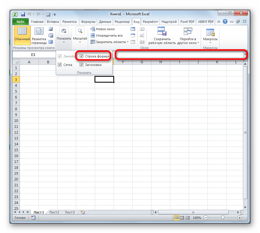
- Переходим во вкладку «Вид». На ленте в блоке инструментов «Показать» около параметра «Строка формул» устанавливаем флажок, если он снят.
- После этих действий строка формул вернется на свое прежнее место. Перезагружать программу или проводить какие-то дополнительные действия не нужно.
Причина 2: настройки параметров Excel
Ещё одной причиной исчезновение ленты может быть её отключение в параметрах Excel. В этом случае её можно включить таким же способом, как было описано выше, а можно произвести включение и тем же путем, которым она была отключена, то есть, через раздел параметров. Таким образом, пользователь имеет выбор.
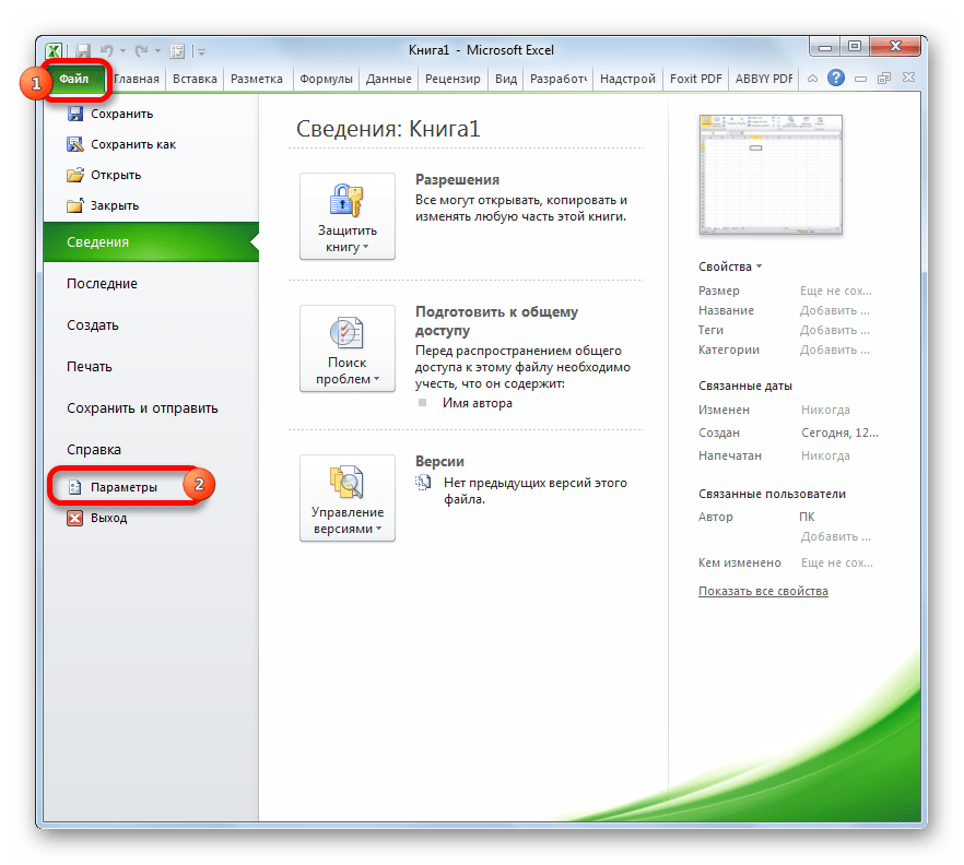
- Переходим во вкладку «Файл». Кликаем по пункту «Параметры».
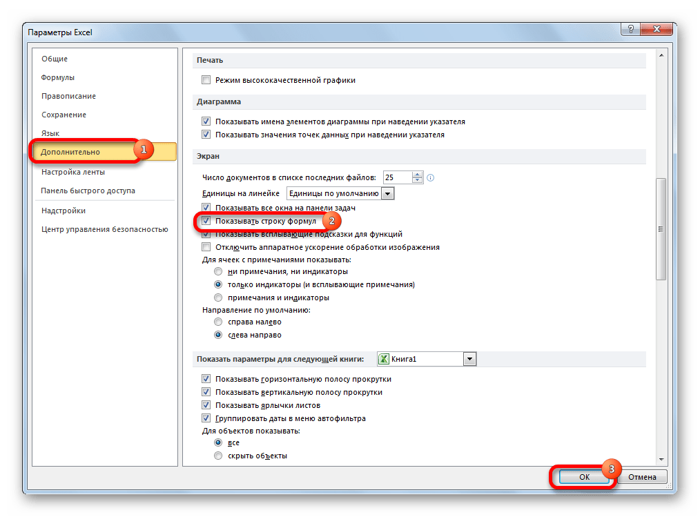
- В открывшемся окне параметров Эксель перемещаемся в подраздел «Дополнительно». В правой части окна этого подраздела ищем группу настроек «Экран». Напротив пункта «Показывать строку формул» устанавливаем галочку. В отличие от предыдущего способа, в этом случае нужно подтвердить изменение настроек. Для этого жмем на кнопку «OK» в нижней части окна. После этого строка формул будет включена снова.
Причина 3: повреждение программы
Как видим, если причина была в настройках, то исправляется она довольно просто. Намного хуже, когда исчезновение строки формул стало следствием сбоя работы или повреждения самой программы, а вышеописанные способы не помогают. В этом случае имеет смысл провести процедуру восстановления Excel.
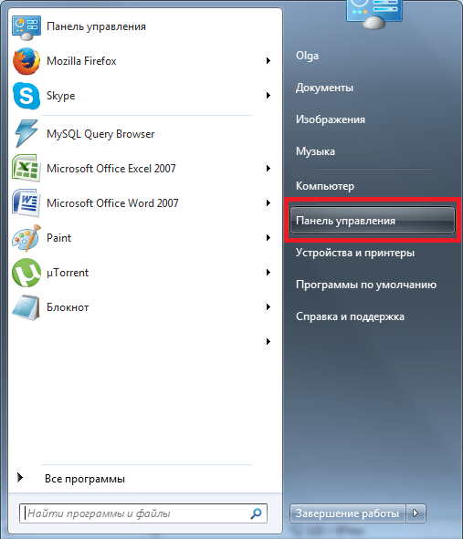
- Через кнопку Пуск переходим в Панель управления.
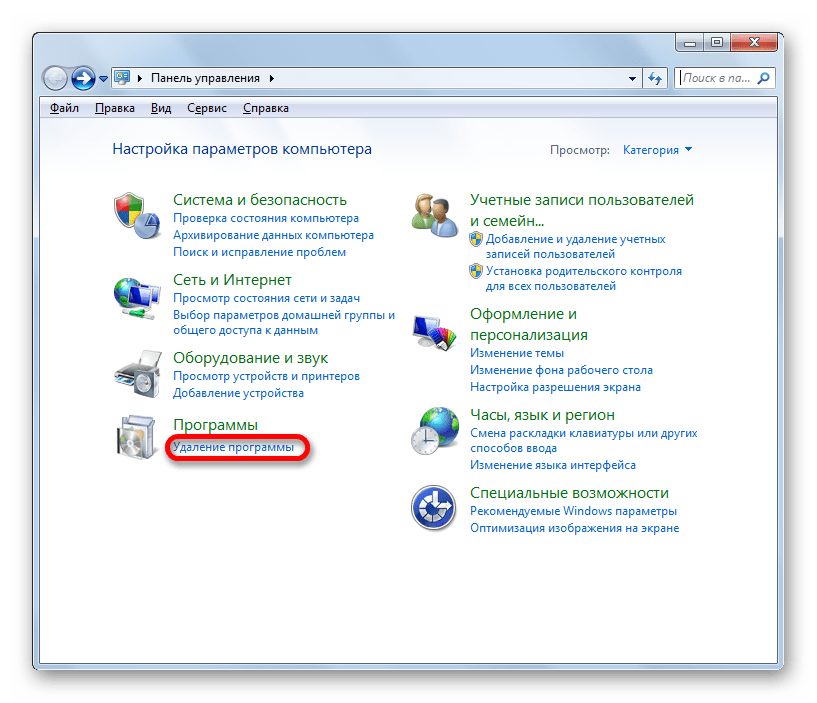
- Далее перемещаемся в раздел «Удаление программ».
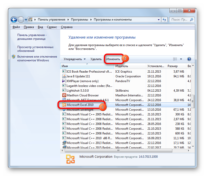
- После этого запускается окно удаления и изменения программ с полным перечнем приложений, установленных на ПК. Находим запись «Microsoft Excel», выделяем её и жмем на кнопку «Изменить», расположенную на горизонтальной панели.
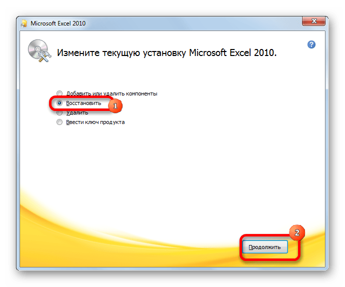
- Запускается окно изменения пакета Microsoft Office. Устанавливаем переключатель в позицию «Восстановить» и жмем на кнопку «Продолжить».
- После этого выполняется процедура восстановления программ пакета Microsoft Office, в том числе и Excel. После её завершения проблем с показом строки формул быть не должно.
Как видим, строка формул может пропасть по двум основным причинам. Если это просто неправильно выставленные настройки (на ленте или в параметрах Excel), то вопрос решается довольно легко и быстро. Если же проблема связана с повреждением или серьезным сбоем в работе программы, то придется пройти процедуру восстановления.

Еще статьи по данной теме:
Помогла ли Вам статья?
Show or Hide Formulas in Excel Using a Keyboard Shortcut, Button or Formula
by Avantix Learning Team | Updated March 7, 2022
Applies to: Microsoft® Excel® 2010, 2013, 2016, 2019, 2021 and 365 (Windows)
You can easily show or hide formulas in a number of ways in Microsoft Excel. You can use a keyboard shortcut, click a button and even use a formula to show formulas. Although you can double-click a cell or press F2 to show the formula in one cell, the first two methods will show formulas in all cells. With the third method, you can view formulas for specific cells.
Recommended article: How to Delete Blank Rows in Excel (5 Fast Ways to Remove Empty Rows)
Do you want to learn more about Excel? Check out our virtual classroom or live classroom Excel courses >
Showing formulas using a keyboard shortcut
You can show or hide formulas using a keyboard shortcut. Press Ctrl + tilde (~) or Ctrl + accent grave (`) to show or hide formulas. The tilde / accent grave key appears on the top left of most keyboards below the Esc key. This shortcut works in all versions of Excel.
Showing formulas using a button
An easy way to show or hide formulas in Excel is to use the Show Formulas button.
To show formulas using a button:
- Click the Formulas tab in the Ribbon.
- In the Formula Auditing group, click Show Formulas. The worksheet will now display with formulas instead of values.
- Click Show Formulas again to hide the formulas.
Below is the Formulas tab in the Ribbon:

Showing formulas using the FORMULATEXT function
You can also use the FORMULATEXT function in a cell to display the formula from another cell as a text string. This is very useful if you want to audit a worksheet and view both values and formulas. The FORMULATEXT function is available in Excel 2013 and later versions.
The syntax for the FORMULATEXT function is =FORMULATEXT(reference) where reference is a cell or a range of cells.
The FORMULATEXT function will return an #N/A error if:
- The formula refers to a cell that does not contain a formula.
- The formula refers to another workbook but the workbook is not open.
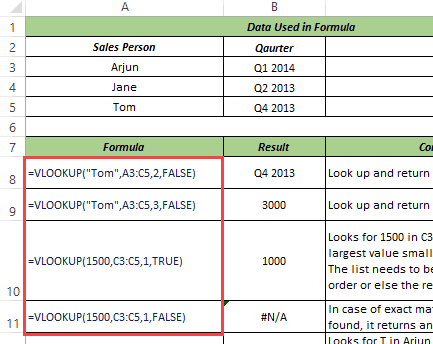
In the following example, we have regular formulas in column C and in column D, we’ve used the FORMULATEXT function:

So in D2, the formula would be =FORMULATEXT(C2).
Bonus: Hiding formulas and locking cells
There is one more method that you can use if you want to really hide formulas and prevent others from unhiding them. You’ll need to choose the Hidden option in the Format Cells dialog box for specific cells and then protect the worksheet.
The first step is to hide the formulas:
- Select the cells with the formulas you wish to hide.
- Right-click the selected cell(s) and choose Format Cells or press Ctrl + 1. The Format Cells dialog appears.
- Click the Protection tab.
- Check Hidden. If you want to protect the cell(s) as well, ensure Locked is checked.
- Click OK. Nothing will appear to occur until you protect the sheet.
Below is the Format Cells dialog box:

The second step is to protect the worksheet:
- Display the worksheet with the cells that have been formatted as Hidden in the Format Cells dialog box.
- Click the Review tab in the Ribbon.
- In the Changes group, click Protect Sheet. A dialog box appears.
- Check or uncheck the desired options (you would usually leave the first two checked).
- Enter a password (you will need to set a password or anyone will be able to unprotect the sheet). Passwords are case sensitive and you should keep a copy of your passwords somewhere else.
- Enter the password again.
- Click OK. All formulas you have marked as Hidden will no longer appear in the Formula Bar.
Below is the Protect Sheet dialog box:

To unhide formulas and unprotect the worksheet:
- Display the desired worksheet.
- Click the Review tab in the Ribbon and click Unprotect Sheet.
- Enter the appropriate password.
- Click OK.
The first two methods are used most often but the last two provide some interesting alternatives.
Subscribe to get more articles like this one
Did you find this article helpful? If you would like to receive new articles, join our email list.
More resources
How to Merge Cells in Excel (4 Ways with Shortcuts)
How to Combine Cells in Excel Using Concatenate (3 Ways)
How to Fill Blank Cells in Excel with a Value from a Cell Above
Automatically Sum Rows and Columns Using the Quick Analysis Tool
How to Use Flash Fill in Excel to Clean or Extract Data (Beginner’s Guide)
Related courses
Microsoft Excel: Intermediate / Advanced
Microsoft Excel: Data Analysis with Functions, Dashboards and What-If Analysis Tools
Microsoft Excel: Introduction to Visual Basic for Applications (VBA)
VIEW MORE COURSES >
Our instructor-led courses are delivered in virtual classroom format or at our downtown Toronto location at 18 King Street East, Suite 1400, Toronto, Ontario, Canada (some in-person classroom courses may also be delivered at an alternate downtown Toronto location). Contact us at info@avantixlearning.ca if you’d like to arrange custom instructor-led virtual classroom or onsite training on a date that’s convenient for you.
Copyright 2023 Avantix® Learning
Microsoft, the Microsoft logo, Microsoft Office and related Microsoft applications and logos are registered trademarks of Microsoft Corporation in Canada, US and other countries. All other trademarks are the property of the registered owners.
Avantix Learning |18 King Street East, Suite 1400, Toronto, Ontario, Canada M5C 1C4 | Contact us at info@avantixlearning.ca
Home / Excel Formulas / How to Hide Formula in Excel
It happens sometimes you send Excel files to others and they made some changes to formulas. Or, sometimes you simply don’t want to show the formula to others.
Hiding a formula is a simple way to do this so that others can’t able to see which formula you have used and how they get calculated.
Now the question is, how can we hide the formula in a cell in Excel?
But before we do that let’s be clear on this point that there are two ways to see a formula from a cell, first, by editing a cell, and second, from the formula bar.
Is there any way you can use to prevent both things? Yes, it’s there. In Excel, there is a simple way for this, and today, I’d like to share with you this simple trick.
Step 1: Un-Protect Worksheet
At this point when you click on a cell, it shows you the entire formula in the formula bar.

- First of all, you need to make sure that your worksheet is unprotected.
- For this, go to the review tab and protect the group.
- If you find an “Unprotect Worksheet” button there, that means your worksheet is protected and you need to unprotect it.

- Click on that button to unprotect it.
If you have the “Protect Sheet” button there that means your worksheet is unprotected. In that case, skip the above steps and start from here.
Step 2: Activate the Hide Formula Option
- Now, select the cell or range of cells, or select all the non-contiguous cells where you want to hide formulas.
- After that, right-click and select the format cells option.

- From the format cells option, go to the Protection tab.
- In the protection tab, you have two checkboxes to mark, the first is locked and the second is hidden.
- Mark both of them and click OK.

These options which you have checked solve both of the problems which we have discussed above.
The locked option restricts the editing of a cell and the hidden option hides a formula from the formula bar. Now the final step is to protect the worksheet.
Step 3: Protect Worksheet
- Right-click on the worksheet tab and then click on “Protect Sheet”.
- Here you need to enter a password. To enter a password (Twice).

- And in the end, click OK.
Now all the cells which you had selected got a formula hidden from the formula bar.

If you send this file to someone they will not be able to see the formula or edit it unless this worksheet is unprotected.
How Do I Find Hidden Formulas?
Once you protect a file using the above steps even you can’t see the formula until you unprotect the worksheet. But if you just want to find them from a protected worksheet where they are, you can use the “Go To Special” option.
- Go to Home Tab -> Editing -> Find & Select -> Go to Special.
- Select the “Formulas” option and it all four sub-option (Numbers, Text, Logical, Errors) and click OK.
- Once you click OK, Excel will select all the cells from the worksheet where you have formulas.
Hide a Formula without Protecting a Worksheet: I’m sure you have this thought in your mind how can I hide a formula without protecting a worksheet? I’m afraid there is no other method for this. You need to go this way. The only possible thing which I know is to create a macro code that runs at the opening of the workbook and hides the formula bar. But, again this is not a permanent solution.
Conclusion
This option not only helps you to hide formulas but also helps if you have any crucial calculations which you want to hide from others.
Until someone has the password, formulas are hidden and safe. I hope this tip will help you to manage your worksheets.
Have you ever tried to hide a formula before? Please share your views with me in the comment section, I’d love to hear from you.
And, make sure to share this tip with your friends.
This tutorial shows how to hide a Formula Bar
Hiding the Formula Bar in Excel comes in useful when a user wants to maximise the workplace in Excel. If you are working with a small screen, want to present a summary of your work or just view more rows without zooming out, than hiding the Formula Bar can give you that extra space you are looking for.
EXCEL METHOD 1. Hide the Formula Bar using a ribbon option
EXCEL
View tab > Show group > Uncheck Formula Bar checkbox
| 1. Select the View tab. |  |
| 2. Click on the Formula Bar checkbox, in the Show group, to unselect the checkbox. |  |
| This image shows the result of these two steps. As you can see the Excel Formula Bar has now been hidden. This will apply to all sheets in the workbook. Note: Excel does not have the ability to hide the Formula Bar in only a specific number of sheets. |
 |
NOTES
This method shows how to hide the Formula Bar by using a checkbox from the excel ribbon, in the View tab. To hide the Formula Bar the checkbox needs to be unchecked and to show the Formula Bar the checkbox needs to be checked. By using this method you can hide the Formula bar in two steps. This example assumes that the Formula Bar is not hidden and therefore the checkbox is originally checked. From the two examples in this tutorial this is the quicker method.
EXCEL METHOD 2. Hide the Formula Bar through Excel Options
EXCEL
VBA METHOD 1. Hide the Formula Bar using VBA
VBA
Sub Hide_the_formula_bar()
‘hide the formula bar
Application.DisplayFormulaBar = False
End Sub
NOTES
Note 1: This VBA code will automatically hide the Formula Bar by setting the Application.DisplayFormulaBar to False. This example assumes that the Formula Bar is originally displayed.
| Related Topic | Description | Related Topic and Description |
|---|---|---|
| Show the Formula Bar | How to show the Formula Bar | |
| Expand the Formula Bar | How to expand the Formula Bar | |
| Collapse the Formula Bar | How to collapse the Formula Bar | |
| What is the Formula Bar? | Explanation about the Formula Bar |
You can better understand what’s going on in your workbooks by showing and highlighting all the formulas in a sheet.
Show/Hide Formulas
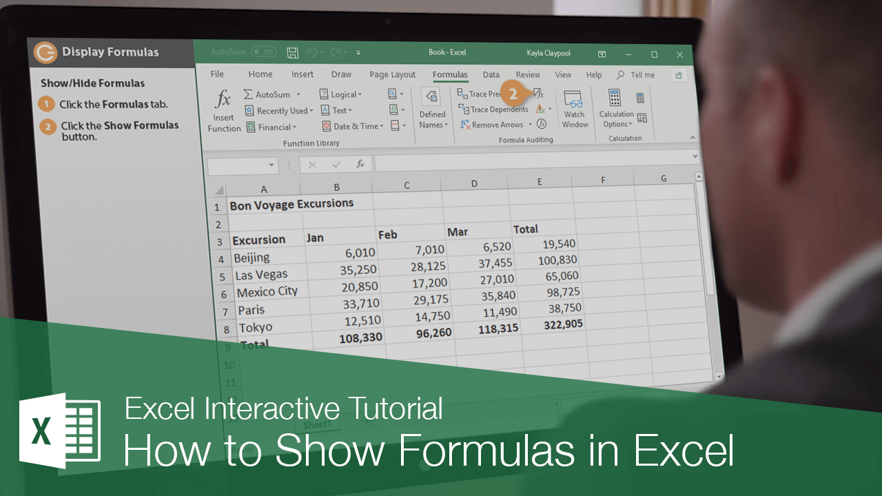
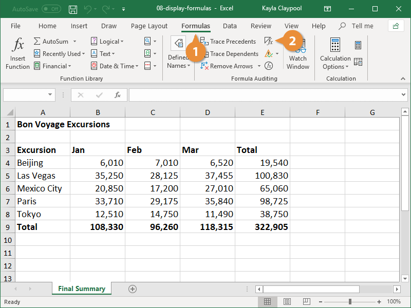
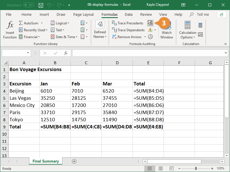
By default, Excel displays the results of formulas in the worksheet instead of showing the actual formulas. However, you can choose to have Excel display the formulas so you can see how they’re put together.
- Click the Formulas tab.
- Click the Show Formulas button.

Formulas are displayed in the worksheet and the columns widen to accommodate the formulas, if necessary.
If you display formulas and then select a cell that contains a formula, colored lines appear around cells that are referenced by the formula.
- Click the Show Formulas button again to hide the formulas.
Formulas are no longer displayed and the columns return to their original sizes.
Highlight Formulas
If you don’t want to see the actual formulas, but want to know which cells contain them, highlight cells with formulas instead.
- Click the Home tab.
- Click the Find & Select button.
- Select Formulas.
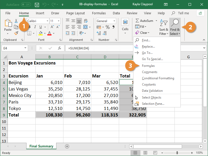
Any cells that contain a formula are highlighted; however, this doesn’t change the cell formatting. When you click any other cell in the worksheet, the highlighted cells are unselected.

FREE Quick Reference
Click to Download
Free to distribute with our compliments; we hope you will consider our paid training.