
Over the years I have seen many things in Excel that have made me go “wow, I won’t do that again in a hurry”. Thankfully as the years have progresses, so has Excel and many of these problem items have been resolved with updates. However, there are still a few things that you should avoid doing in Excel or stop doing altogether. One of these is the use of the popular Merge cells in Excel formatting option. I beg of you, do not merge cells in Excel
Merging cells in Excel cause problems with sorting and moving data. In this article we are going to look at the types of problems that you will encounter when you use merged cells and of course, a solution too 😊
Why you should not Merge cells in Excel
Pretty and all as you would like your spreadsheets to be, if you merge cells in Excel it can cause many different problems. First, if you are ensuring your workbook is accessible for people of all abilities, merging cells may skew layout to a screen reader and users may be given the information in the wrong context. Best practice on spreadsheet accessibility advises against the use of Merged Cells.
You might also find when you merge cells in Excel, some of your formula might not give you the value you expected. This is because merging cells loses the integrity of columns and rows.
Consider the following. We have two columns of data. We have totaled these columns using the SUM function. You can see from the image the SUM formula takes row 1 to row 6.

Let’s say we now merge the column A and B for row 1, Excel will see the value in the left most column. In this case, column A. The result is that column A now includes the 1990 which should be in column B.

Consider the following table of data. This table contains 3 columns merged for 1 row in the table.

If we were to try and sort this table by any of the Products, we would get an error as there are merged columns which breaks the traditional column structure.

Alternative Solution for Merged Cells in Excel.
Do not despair. We can easily apply a different formatting that will keep the appearance of merged cells, yet the cells won’t be merged. That way your workbook and spreadsheet remain pretty. After-all you don’t want to lose that look right! And we can continue to work with our data with out the error we discussed above.
To format cells so there appear as merged, select the cells. Right Click and select Format Cells.

This will open the format cells window. Select the Alignment tab.

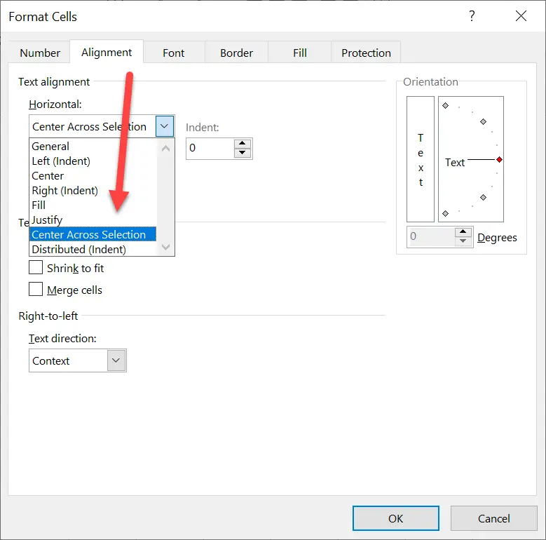
From the Horizontal drop down, select Center Across Selection. The contents of the cell will then appear as if it was merged.

This only works from Left to Right and Excel will assume the value to be contained within the left most column.
Now if we try and sort the table, we do not face the same problem and the data sorts with ease.

Locating Merged Cells in Excel
Now you have read the article you are convinced merged cells are a big no in Excel. That was easy, Job done. But wait. The next problem is locating these cells so we can fix them. To do this, we are going to use Excels Find option.
The keyboard shortcut CTRL + F will open the Find and Replace window.

Once we open Find, we can select Options. Among other things this will allow us select between different formats. Select Format to open the Find Format window.

In the Find Format window, select the Alignment tab and select Merge cells. We do not need to select any other options as we are only searching for merged cells. Pressing OK will close the Find Format box and return us to the Find and Replace window.

By selecting Find All will list all the merged cells. Selecting any of these from the list will make it the active cell in the workbook. This allows you quickly navigate to merged cells.

You can repair your workbook or try converting the table to range
by Sagar Naresh
Sagar is a web developer and technology journalist. Currently associated with WindowsReport and SamMobile. When not writing, he is either at the gym sweating it out or playing… read more
Updated on December 13, 2022
Reviewed by
Alex Serban

After moving away from the corporate work-style, Alex has found rewards in a lifestyle of constant analysis, team coordination and pestering his colleagues. Holding an MCSA Windows Server… read more
- Merging cells makes a dataset look presentable and properly formatted.
- However, often you won’t be able to merge cells because the workbook is protected or it is shared.
- You can first try to remove the protection or convert the table to a range.
XINSTALL BY CLICKING THE DOWNLOAD FILE
This software will repair common computer errors, protect you from file loss, malware, hardware failure and optimize your PC for maximum performance. Fix PC issues and remove viruses now in 3 easy steps:
- Download Restoro PC Repair Tool that comes with Patented Technologies (patent available here).
- Click Start Scan to find Windows issues that could be causing PC problems.
- Click Repair All to fix issues affecting your computer’s security and performance
- Restoro has been downloaded by 0 readers this month.
MS Excel is a powerful tool that comes with a plethora of great features to represent or get meaningful information out of a dataset. Merging cells is another great feature when you want to format the heading or center just to present the dataset in a proper manner.
However, there are reports where users have complained that for them, Excel cells are not merging. In this guide, we will give you five solutions that will help you get rid of the issue. Let us check them out.
Why aren’t the MS Excel cells merging?
After some research, we have found a few reasons that might be restricting you from merging cells in your MS Excel spreadsheet:
- Cells are within a table: This is one of the most common reasons because of why you are coming across MS Excel cells that are not merging issues. Excel table does not allow you to merge cells that are inside a table.
- Your worksheet is protected: For safety reasons and to avoid people from editing your worksheet, chances are the worksheet that isn’t allowing you to merge cells is protected.
- Your worksheet is shared: Do note that along with the protected worksheet, a shared worksheet will also not allow you to merge cells in Excel.
These are the three main reasons why you are facing MS Excel cells not merging issues.
What can I do if Excel cells are not merging?
Here are a few things that you can do before applying the advanced solutions:
- Perform a simple restart. Often if the program fails to load all its files properly, then it can throw up multiple errors.
- Check if you are running the latest version of MS Excel on your PC. This ensures that this error isn’t because of an old version or compatibility issue.
- Make sure that the worksheet that you are working on isn’t corrupt and does not have incompatible values.
Now, let us take a look at the solutions that will help you resolve this problem.
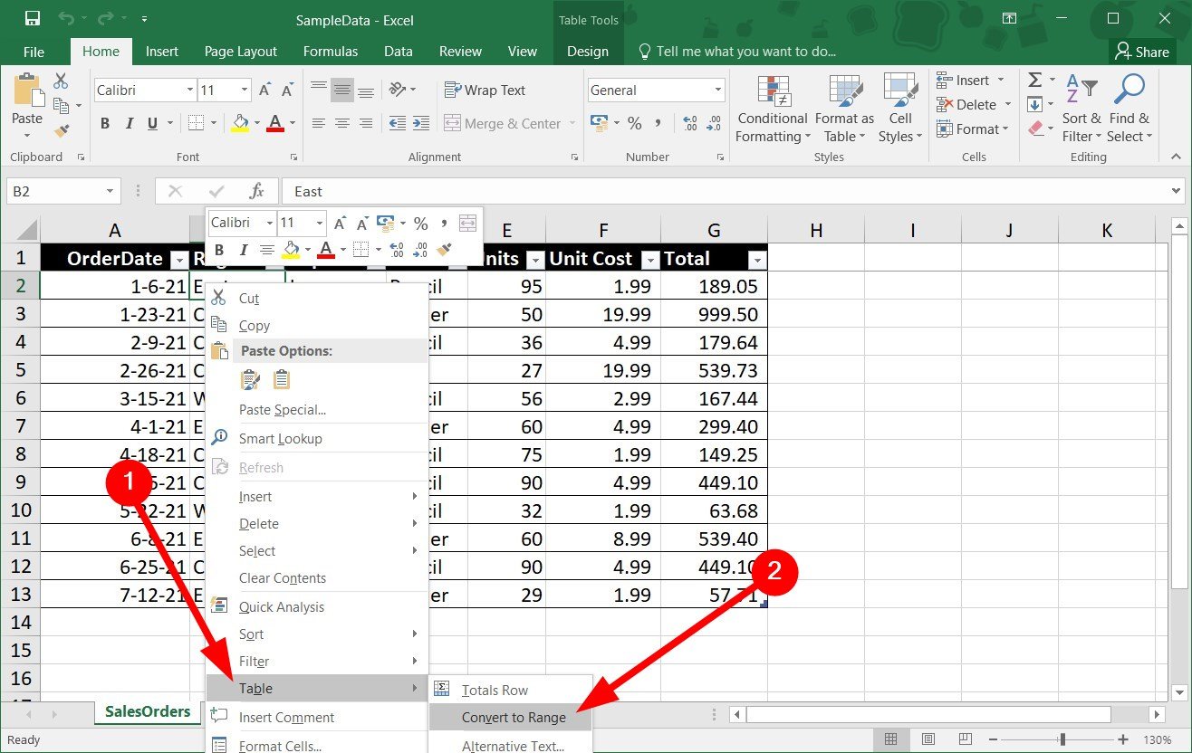
- Select the entire table or click on any cell within the table.
- Right-click, select Table, and click on Convert to Range option from the context menu.

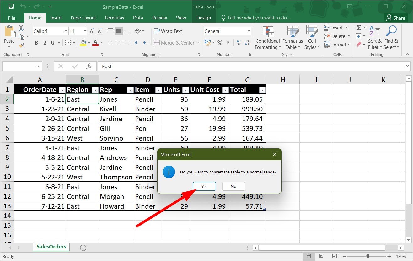
- Excel will show a confirmation window Do you want to convert the table to a normal range?
- Click Yes.
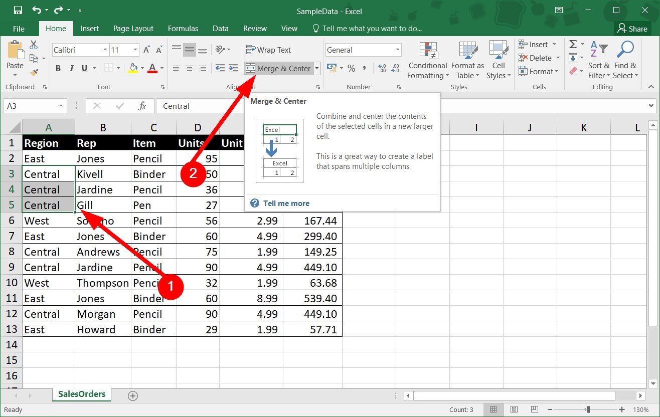
- Now select the cells that you wish to merge.
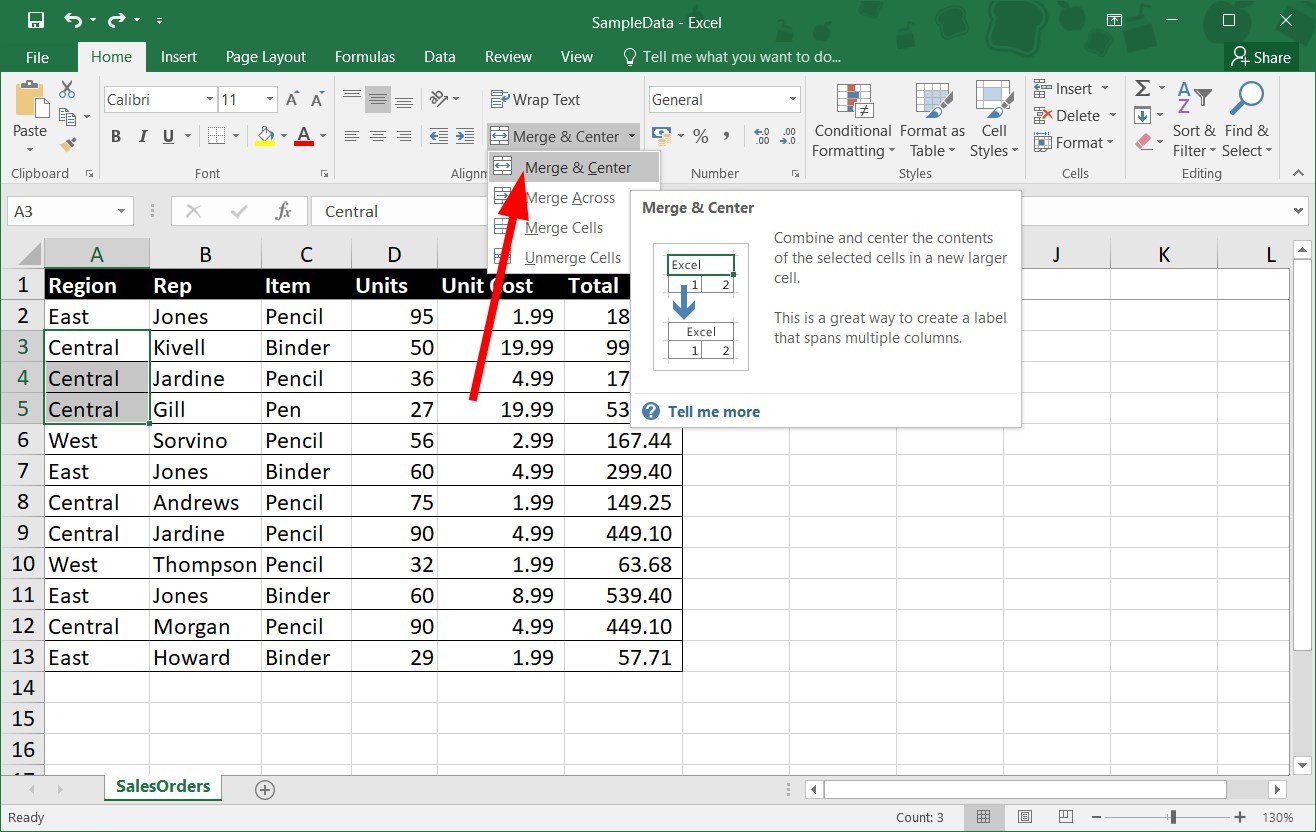
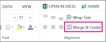
- Click on Merge & Center button at the top menu bar in the Home tab.
- Select Merge & center again from the drop-down menu.
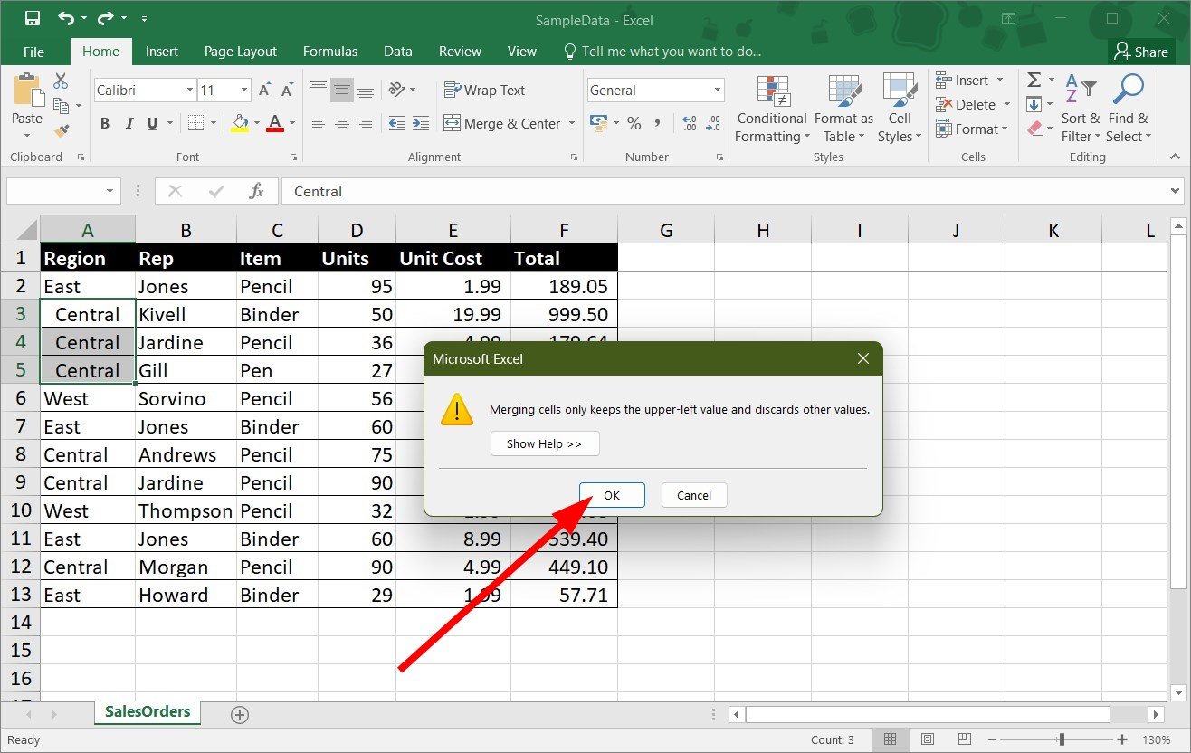
- A pop will show you Merging cells only keeps the upper-left value and discards other values warning. Click Yes.
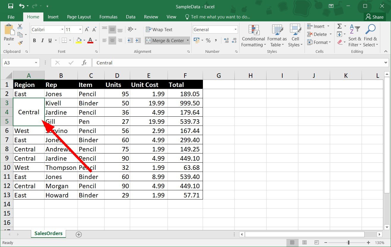
- You will see your selected cells are now merged.
2. Unprotect your workbook
- Open your workbook.
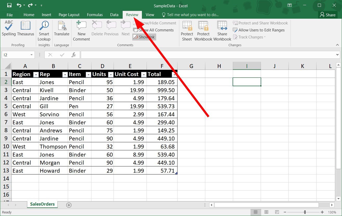
- Click on the Review tab.
- Click on Unprotect Worksheet and Unprotect Workbook.
- Select the cells that you wish to merge.
- Select Merge & Center button at the top menu bar in the Home tab.
- Click on Merge & center again from the drop-down menu.
- A pop will show you Merging cells only keeps the upper-left value and discards other values warning. Click Yes.
- You will see your selected cells are now merged.

The protected workbook will prevent you from editing, let alone merging cells. In such a case, you can follow the steps above and unprotect your cells.
Some PC issues are hard to tackle, especially when it comes to corrupted repositories or missing Windows files. If you are having troubles fixing an error, your system may be partially broken.
We recommend installing Restoro, a tool that will scan your machine and identify what the fault is.
Click here to download and start repairing.
Then you can follow solution 1 and convert the data to the range and then apply the merge function to merge the selected cells.
- Excel Running Slow? 4 Quick Ways to Make It Faster
- Fix: Excel Stock Data Type Not Showing
- Best Office Add-Ins: 15 Picks That Work Great in 2023
- Errors Were Detected While Saving [Excel Fix Guide]
- Excel Not Scrolling Smoothly: Fix It in 5 Simple Steps
3. Unshare your workbook
- Open your workbook.
- Click on the Review tab.
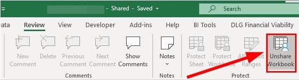
- Under the Protect section, click on Unshare workbook option.

- Now you can go ahead and merge the cells.
4. Disable Add-Ins
- Open your workbook.
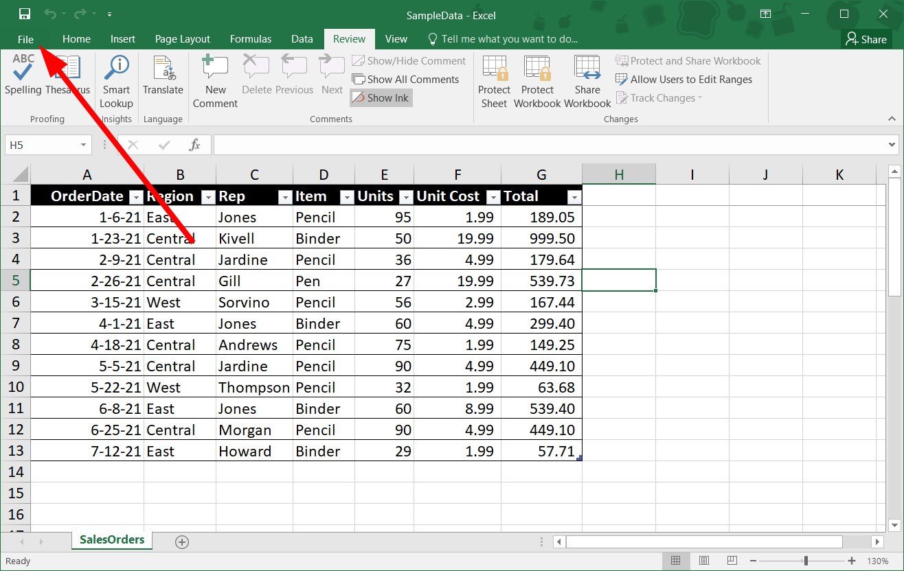
- Click on the File option at the top Menu bar.
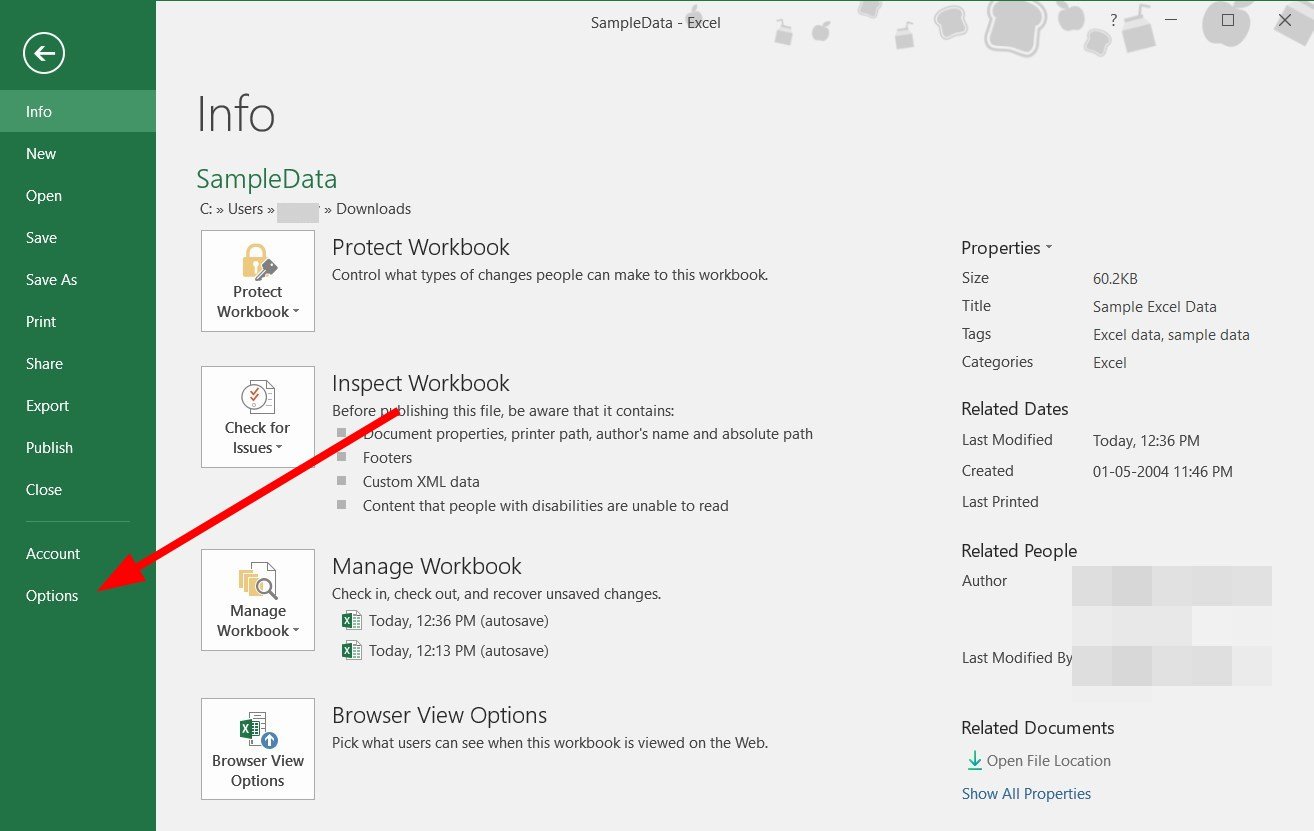
- Select Options from the left panel.

- Click on Add-in.

- Make sure that the add-ins are disabled.
- Go back to your worksheet and check if you can merge cells or not.

Often add-ins can interfere with the smooth functioning of the MS Excel program. While we install add-ins to enhance the functionality of the program, they can cause issues such as Excel cells not merging problems.
In this case, we would suggest you disable all the add-ins by following the above steps and then trying to merge cells in your workbook.
5. Repair your workbook
- Launch MS Excel.
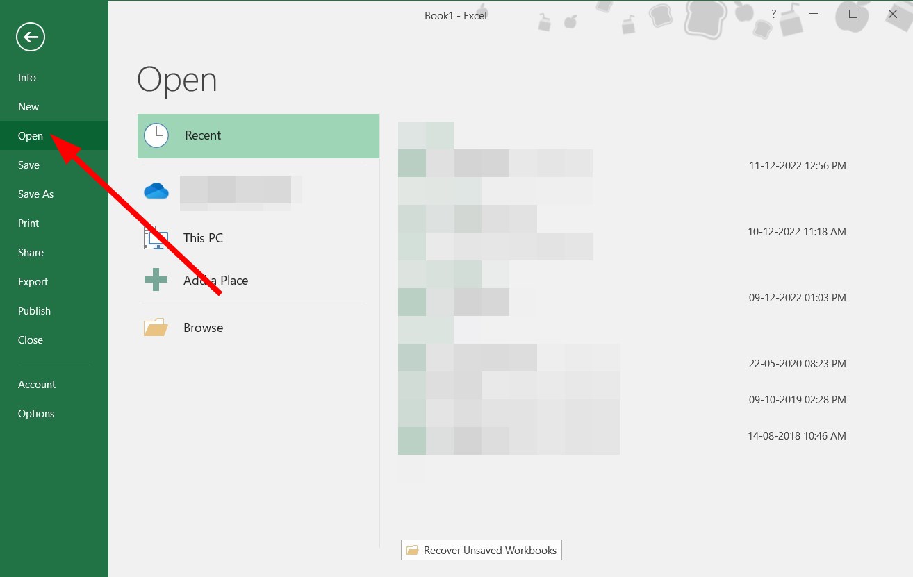
- Click on File.
- Click on Open.
- Select your file and from the Tools drop-down menu, select the Open and Repair option.
- Select Repair on the message that pops up.
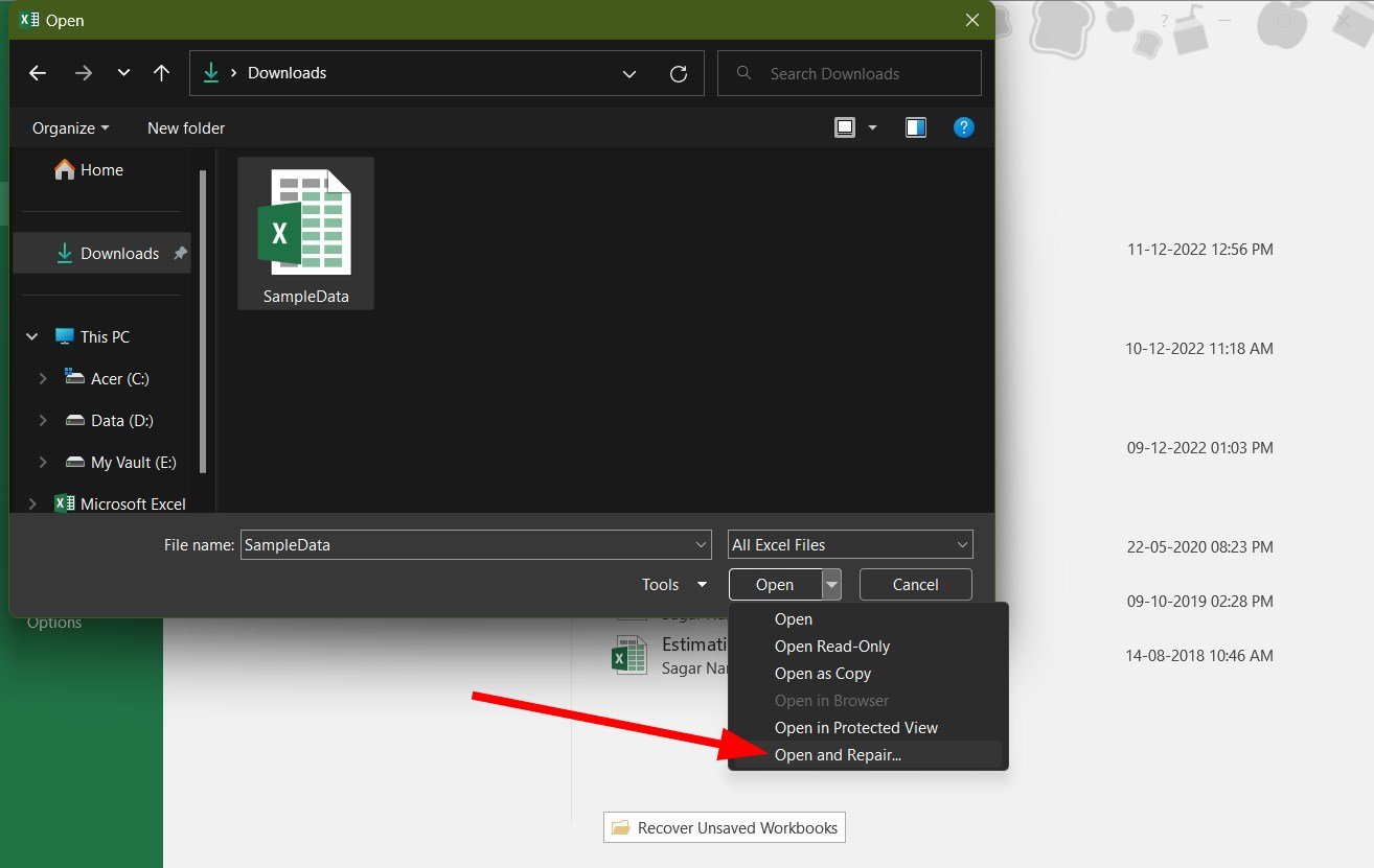
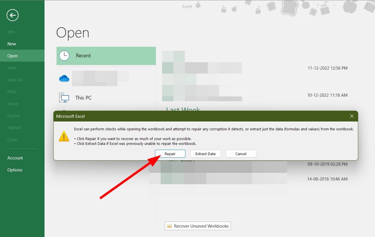
Often workbooks get corrupted, or data in them get lost, which could be an issue if you aren’t able to merge cells in Excel. Simply follow the above steps, repair your workbook, and check if this resolves the issue or not.
These are some of the best solutions to apply when cells are not merging in MS Excel. Well, you will come across other issues with MS Excel as well.
For users facing Excel won’t scroll down errors, we have a guide that lists some effective solutions to resolve it. We also have a guide on the Excel toolbar missing to fix the issue.
Moreover, if you want to know how you can open two Excel side by side to improve efficiency, you can refer to our guide. Also, did you know that you can open multiple Excel files at once?
We also have a dedicated guide for those who aren’t able to open Excel on their Windows 11 PCs. Let us know in the comments below which one of the above solutions helped you fix the cells that are not merging in MS Excel.
Still having issues? Fix them with this tool:
SPONSORED
If the advices above haven’t solved your issue, your PC may experience deeper Windows problems. We recommend downloading this PC Repair tool (rated Great on TrustPilot.com) to easily address them. After installation, simply click the Start Scan button and then press on Repair All.
![]()
Newsletter
Merge and unmerge cells
You can’t split an individual cell, but you can make it appear as if a cell has been split by merging the cells above it.

Merge cells
-
Select the cells to merge.
-
Select Merge & Center.
Important: When you merge multiple cells, the contents of only one cell (the upper-left cell for left-to-right languages, or the upper-right cell for right-to-left languages) appear in the merged cell. The contents of the other cells that you merge are deleted.
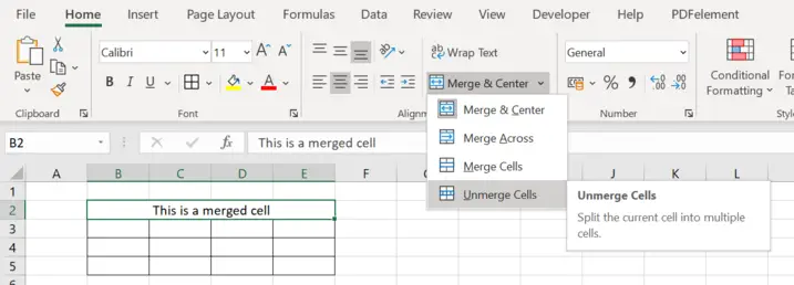
Unmerge cells
-
Select the Merge & Center down arrow.
-
Select Unmerge Cells.
Important:
-
You cannot split an unmerged cell. If you are looking for information about how to split the contents of an unmerged cell across multiple cells, see Distribute the contents of a cell into adjacent columns.
-
After merging cells, you can split a merged cell into separate cells again. If you don’t remember where you have merged cells, you can use the Find command to quickly locate merged cells.
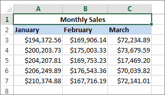
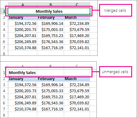
Merging combines two or more cells to create a new, larger cell. This is a great way to create a label that spans several columns.
In the example here, cells A1, B1, and C1 were merged to create the label “Monthly Sales” to describe the information in rows 2 through 7.
Merge cells
Merge two or more cells by following these steps:
-
Select two or more adjacent cells you want to merge.
Important: Ensure that the data you want to retain is in the upper-left cell, and keep in mind that all data in the other merged cells will be deleted. To retain any data from those other cells, simply copy it to another place in the worksheet—before you merge.
-
On the Home tab, select Merge & Center.

Tips:
-
If Merge & Center is disabled, ensure that you’re not editing a cell—and the cells you want to merge aren’t formatted as an Excel table. Cells formatted as a table typically display alternating shaded rows, and perhaps filter arrows on the column headings.
-
To merge cells without centering, click the arrow next to Merge and Center, and then click Merge Across or Merge Cells.
Unmerge cells
If you need to reverse a cell merge, click onto the merged cell and then choose Unmerge Cells item in the Merge & Center menu (see the figure above).
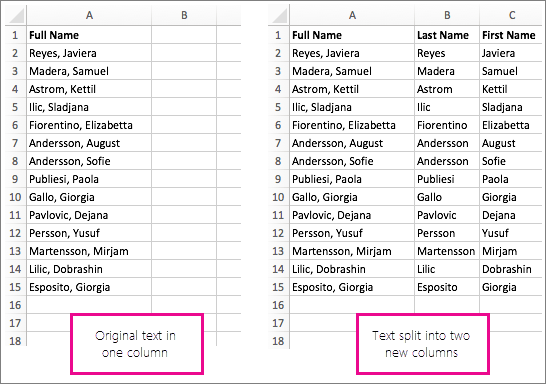
Split text from one cell into multiple cells
You can take the text in one or more cells, and distribute it to multiple cells. This is the opposite of concatenation, in which you combine text from two or more cells into one cell.
For example, you can split a column containing full names into separate First Name and Last Name columns:
Follow the steps below to split text into multiple columns:
-
Select the cell or column that contains the text you want to split.
-
Note: Select as many rows as you want, but no more than one column. Also, ensure that are sufficient empty columns to the right—so that none of your data is deleted. Simply add empty columns, if necessary.
-
Click Data >Text to Columns, which displays the Convert Text to Columns Wizard.
-
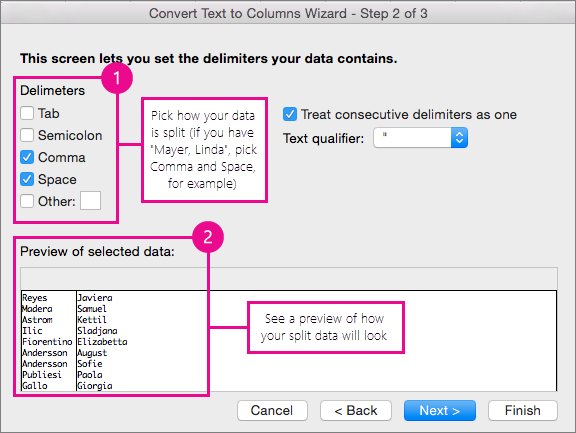
Click Delimited > Next.
-
Check the Space box, and clear the rest of the boxes. Or, check both the Comma and Space boxes if that is how your text is split (such as «Reyes, Javiers», with a comma and space between the names). A preview of the data appears in the panel at the bottom of the popup window.
-
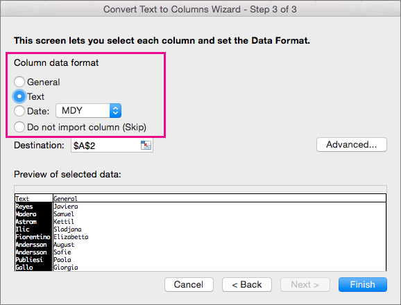
Click Next and then choose the format for your new columns. If you don’t want the default format, choose a format such as Text, then click the second column of data in the Data preview window, and click the same format again. Repeat this for all of the columns in the preview window.
-
Click the
button to the right of the Destination box to collapse the popup window. -
Anywhere in your workbook, select the cells that you want to contain the split data. For example, if you are dividing a full name into a first name column and a last name column, select the appropriate number of cells in two adjacent columns.
-
Click the
button to expand the popup window again, and then click the Finish button.
 button to the right of the Destination box to collapse the popup window.
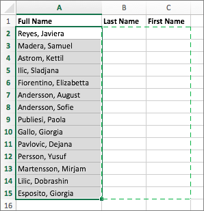
 button to expand the popup window again, and then click the Finish button.
Merging combines two or more cells to create a new, larger cell. This is a great way to create a label that spans several columns. For example, here cells A1, B1, and C1 were merged to create the label “Monthly Sales” to describe the information in rows 2 through 7.
Merge cells
-
Click the first cell and press Shift while you click the last cell in the range you want to merge.
Important: Make sure only one of the cells in the range has data.
-
Click Home > Merge & Center.
If Merge & Center is dimmed, make sure you’re not editing a cell or the cells you want to merge aren’t inside a table.
Tip: To merge cells without centering the data, click the merged cell and then click the left, center or right alignment options next to Merge & Center.
If you change your mind, you can always undo the merge by clicking the merged cell and clicking Merge & Center.
Unmerge cells
To unmerge cells immediately after merging them, press Ctrl + Z. Otherwise do this:
-
Click the merged cell and click Home > Merge & Center.
The data in the merged cell moves to the left cell when the cells split.
Need more help?
You can always ask an expert in the Excel Tech Community or get support in the Answers community.
See Also
Overview of formulas in Excel
How to avoid broken formulas
Find and correct errors in formulas
Excel keyboard shortcuts and function keys
Excel functions (alphabetical)
Excel functions (by category)
Need more help?
Merged cells are one of the most popular options used by beginner spreadsheet users.
But they have a lot of drawbacks that make them a not so great option.
In this post, I’ll show you everything you need to know about merged cells including 8 ways to merge cells.
I’ll also tell you why you shouldn’t use them and a better alternative that will produce the same visual result.
What is a Merged Cell
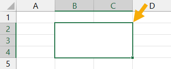
A merged cell in Excel combines two or more cells into one large cell. You can only merge contiguous cells that form a rectangular shape.
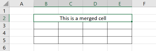
The above example shows a single merged cell resulting from merging 6 cells in the range B2:C4.
Why You Might Merge a Cell
Merging cells is a common technique used when a title or label is needed for a group of cells, rows or columns.
When you merge cells, only the value or formula in the top left cell of the range is preserved and displayed in the resulting merged cell. Any other values or formulas are discarded.
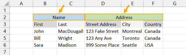
The above example shows two merged cells in B2:C2 and D2:F2 which indicates the category of information in the columns below. For example the First and Last name columns are organized with a Name merged cell.
Why is the Merge Command Disabled?
On occasion, you might find the Merge & Center command in Excel is greyed out and not available to use.
There are two reasons why the Merge & Center command can become unavailable.
- You are trying to merge cells inside an Excel table.
- You are trying to merge cells in a protected sheet.
Cells inside an Excel table can not be merged and there is no solution to enable this.
If most of the other commands in the ribbon are greyed out too, then it’s likely the sheet is protected. In order to access the Merge option, you will need to unprotect the worksheet.
This can be done by going to the Review tab and clicking the Unprotect Sheet command.
If the sheet has been protected with a password, then you will need to enter it in order to unprotect the sheet.
Now you should be able to merge cells inside the sheet.
Merged Cells Only Retain the Top Left Values
Warning before you start merging cells!
If the cells contain data or formulas, then you will lose anything not in the upper left cell.
A warning dialog box will appear telling you Merging cells only keeps the upper-left value and discards other values.
The above example shows the result of merging cells B2:C4 which contains text data. Only the data from cell B2 remains in the resulting merged cells.
If no data is present in the selected cells, then no warning will appear when trying to merge cells.
8 Ways to Merge a Cell
Merging cells is an easy task to perform and there are a variety of places this command can be found.
Merge Cells with the Merge & Center Command in the Home Tab
The easiest way to merge cells is using the command found in the Home tab.
- Select the cells you want to merge together.
- Go to the Home tab.
- Click on the Merge & Center command found in the Alignment section.
Merge Cells with the Alt Hotkey Shortcut
There is an easy way to access the Home tab Merge and Center command using the Alt key.
Press Alt H M C in sequence on your keyboard to use the Merge & Center command.
Merge Cells with the Format Cells Dialog Box
Merging cells is also available from the Format Cells dialog box. This is the menu which contains all formatting options including merging cells.
You can open the Format Cells dialog box a few different ways.
- Go to the Home tab and click on the small launch icon in the lower right corner of the Alignment section.
- Use the Ctrl + 1 keyboard shortcut.
- Right click on the selected cells and choose Format Cells.
Go to the Alignment tab in the Format Cells menu then check the Merge cells option and press the OK button.
Merge Cells with the Quick Access Toolbar
If you use the Merge & Center command a lot, then it might make sense to add it to the Quick Access Toolbar so it’s always readily available to use.
Go to the Home tab and right click on the Merge & Center command then choose Add to Quick Access Toolbar from the options.
This will add the command to your QAT which is always available to use.
A nice bonus that comes with the quick access command is it gets its own hotkey shortcut based on its position in the QAT. When you press the Alt key, Excel will show you what key to press next in order to access the command.
In the above example, the Merge and Center command is the third command in the QAT so the hotkey shortcut is Alt 3.
Merge Cells with Copy and Paste
If you have a merged cell in your sheet already then you can copy and paste it to create more merged cells. This will produce merged cells with the exact same dimensions.
Copy a merged cell using Ctrl + C then paste it into a new location using Ctrl + V. Just make sure the paste area doesn’t overlap an existing merged cell.
Merge Cells with VBA
Sub MergeCells()
    Range("B2:C4").Merge
End Sub
The basic command for merging cells in VBA is quite simple. The above code will merge cells B2:C4.
Merge Cells with Office Scripts
function main(workbook: ExcelScript.Workbook) {
	let selectedSheet = workbook.getActiveWorksheet();
	selectedSheet.getRange("B2:C4").merge(false);
	selectedSheet.getRange("B2:C4").getFormat().setHorizontalAlignment(ExcelScript.HorizontalAlignment.center);
}
The above office script will merge and center the range B2:C4.
Merge Cells inside a PivotTable
We can’t make this change for the selected cells because it will affect a PivotTable. Use the field list to change the report. If you are trying to insert or delete cells, move the PivotTable and try again.
If you try to use the Merge and Center command inside a Pivot Table, you will be greeted with the above error message.
You can’t use the Merge & Center command inside a PivotTable, but there is a way to merge cells in the PivotTable options menu.
In order to avail of this option, you will first need to make sure your Pivot Table is in the tabular display mode.
- Select a cell inside your PivotTable.
- Go to the Design tab.
- Click on Report Layout.
- Choose Show in Tabular Form.
Your pivot table will now be in the tabular form where each field you add to the Rows area will be in its own column with data in a displayed in a single row.
Now you can enable the option to show merge cells inside the pivot table.
- Select a cell inside your PivotTable.
- Go to the PivotTable Analyze tab.
- Click on Options.
This will open up the PivotTable Options menu.
Enable the Merge and center cells with labels setting in the PivotTable Options menu.
- Click on the Layout & Format tab.
- Check the Merge and center cells with labels option.
- Press the OK button.
Now as you expand and collapse fields in your pivot table, fields will merge when they have a common label.
10 Ways to Unmerge a Cell
Unmerging a cell is also quick and easy. Most methods involve the same steps as used to merge the cell, but there are a few extra methods worth knowing.
Unmerge Cells with the Home Tab Command
This is the same process as merging cells from the Home tab command.
- Select the merged cells to unmerge.
- Go to the Home tab.
- Click on the Merge & Center command.
Unmerge Cells with the Format Cells Menu
You can unmerge cells from the Format Cells dialog box as well.
Press Ctrl + 1 to open the Format Cells menu then go to the Alignment tab then uncheck the Merge cells option and press the OK button.
Unmerge Cells with the Alt Hot Key Shortcut
You can use the same Alt hot key combination to unmerge a merged cell. Select the merged cell you want to unmerge then press Alt H M C in sequence to unmerge the cells.
Unmerge Cells with Copy and Paste
You can copy the format from a regular single cell to unmerge merged cells.
Find a single cell and use Ctrl + C to copy it, then select the merged cells and press Ctrl + V to paste the cell.
You can use the Paste Special options to avoid overwriting any data when pasting. Press Ctrl + Alt + V then select the Formats option.
Unmerge Cells with the Quick Access Toolbar
This is a great option if you have already added the Merge & Center command to the quick access toolbar previously.
All you need to do is select the merged cells and click on the command or use the Alt hot key shortcut.
Unmerge Cells with the Clear Formats Command
Merged cells are a type of format, so it’s possible to unmerge cells by clearing the format from the cell.
- Select the merged cell to unmerge.
- Go to the Home tab.
- Click on the right part of the Clear button found in the Editing section.
- Select Clear Formats from the options.
Unmerge Cells with VBA
Sub UnMergeCells()
    Range("B2:C4").UnMerge
End Sub
Above is the basic command for unmerging cells in VBA. This will unmerge cells B2:C4.
Unmerge Cells with Office Scripts
Most methods of merging a cell can be performed again to unmerge cells like a toggle switch to merge or unmerge.
However the code in office scripts doesn’t work like this and instead, you will need to remove formatting to unmerge.
function main(workbook: ExcelScript.Workbook) {
	let selectedSheet = workbook.getActiveWorksheet();
	selectedSheet.getRange("B2:C4").clear(ExcelScript.ClearApplyTo.formats);
}
The above code will clear the format in cells B2:C4 and unmerge any merged cells it contains.
Unmerge Cells with the Accessibility Pane
Merged cells create problems for screen readers which is an accessibility issue. Because of this, they are flagged in the Accessibility window pane.
If you know the location of the merged cells, you can select them and go to the Review tab then click on the lower part of the Check Accessibility button and choose Unmerge Cells.
If you don’t know where all the merged cells are, you can open up the accessibility pane and it will show you where there are and you will be able to unmerge them one by one.
Go to the Review tab and click on the top part of the Check Accessibility command to launch the accessibility window pane.
This will show a Merged Cells section which you can expand to see all merged cells in the workbook. Click on the address and Excel will take you to that location.
Click on the downward chevron icon to the right of the address and the Unmerge option can be selected.
Unmerge Cells inside a PivotTable
To unmerge cells inside a pivot table, you just need to disable the setting in the pivot table options menu.
Now you can enable the option to show merge cells inside the pivot table.
- Select a cell inside your PivotTable.
- Go to the PivotTable Analyze tab.
- Click on Options.
- Click on the Layout & Format tab.
- Uncheck the Merge and center cells with labels option.
- Press the OK button.
Merge Multiple Ranges in One Step
In Excel, you can select multiple non-continuous ranges in a sheet by holding the Ctrl key. A nice consequence of this is you can convert these multiple ranges into merged cells in one step.
Hold the Ctrl key while selecting multiple ranges with the mouse. When you’re finished selecting the ranges you can release the Ctrl key and then go to the Home tab and click on the Merge & Center command.
Each range will become its own merged cell.
Combine Data Before Merging Cells
Before you merge any cells which contain data, it’s advised to combine the data since only the data in the top left cell is preserved when merging cells.
There are a variety of ways to do this, but using the TEXTJOIN function is among the easiest and most flexible as it will allow you to separate each cell’s data using a delimiter if needed.
= TEXTJOIN ( ", ", TRUE, B2:C4 )The above formula will join all the text in range B2:C4 going from left to right and then top to bottom. Text in each cell is separated with a comma and space.
Once you have the formula result, you can copy and paste it as a value so that the data is retained when you merge the cells.
How to Get Data from Merged Cells in Excel
A common misconception is that each cell of in the merged range contains the data entered inside.
In fact, only the top left cell will contain any data.
In the above example, the formula references the top left value in the merged range. The result returned is what is seen in the merged range.
In this example, the formula references a cell that is not the top left most cell in the merged range. The result is 0 because this cell is empty and contains no value.
In order to extract data from a merged range, you will always need to reference the top left most cell of the range. Fortunately, Excel automatically does this for you when you select the merged cell in a formula.
How to Find Merged Cells in a Workbook
If you create a bunch of merged cells, you might need to find them all later. Thankfully it’s not a painful process.
This can be done using the Find & Select command.
Go to the Home tab and click on the Find & Select button found in the Editing section, then choose the Find option. This will open the Find and Replace menu
You can also use the Ctrl + F keyboard shortcut.
You don’t need to enter any text to find, you can use this menu to find cells formatted as merged cells.
- Click on the Format button to open the Find Format menu.
- Go to the Alignment tab.
- Check the Merge cells option.
- Press the OK button in the Find Format menu.
- Press the Find All or Find Next button in the Find and Replace menu.
Unmerge All Merged Cells
Fortunately, unmerging all merged cells in a sheet is very easy.
- Select the entire sheet. You can do this two ways.
- Click on the select all button where the column headings meet the row headings.
- Press Ctrl + A on your keyboard.
- Go to the Home tab.
- Press the Merge & Center command.
This will unmerge all the merged cells and leave all the other cells unaffected.
Why You Shouldn’t Merge Cells
There are a lot of reasons why you shouldn’t merge cells.
- You can’t sort data with merged cells.
- You can’t filter data with merged cells.
- You can’t copy and paste values into merged cells.
- It will create accessibility problems for screen readers by changing the order in which text should be read.
This isn’t an exhaustive list, there are likely many more you will come across should you choose to merge cells.
Alternative to Merging a Cell
Good news!
There is a much better alternative than merging cells.
This alternative has none of the negative features that come with merging cells but will still allow you to achieve the same visual look of a merged cell.
It will allow you to display text centered across a range of cells without merging the cells.
Unfortunately, this technique will only work horizontally with one row of cells. There is no option to do something similar with a vertical range of cells.
Select the horizontal range of cells that you would like to center your text across. The first cell should contain the text which is to be centered while the remaining cells should be empty.
This example shows text in cell B2 and the range B2:C2 is selected as the range to center across.
Go to the Home tab and click on the small launch icon in the lower right corner of the Alignment section. This will open up the Format Cells dialog box with the Alignment tab active.
You can also press Ctrl + 1 to open the Format Cells dialog box and navigate to the Alignment tab.
Select Center Across Selection from the Horizontal dropdown options in the Text alignment section.
The text will now appear as though it occupies all cells but it will only exist in the first cell of the centering selection and each cell is still separate.
Pros
- The text appears centered across the selected range similar to a merged cell.
- No negative effects from merged cells.
- Can be used inside an Excel table.
Cons
- Can not center across a vertical range of cells.
Conclusions
There are lots of ways to merge cells in Excel. You can also easily unmerge cells too if you need to.
There are many things to consider when merging cells in Excel.
As you have seen, there are lots of pitfalls to merged cells that you should consider before implementing them in your workbooks.
Do you have a favorite merge method or warning about the dangers of merged cells that are not listed in the post? Let me know about it in the comments.
About the Author
John is a Microsoft MVP and qualified actuary with over 15 years of experience. He has worked in a variety of industries, including insurance, ad tech, and most recently Power Platform consulting. He is a keen problem solver and has a passion for using technology to make businesses more efficient.

PerfectXL Risk Eliminator
It is so tempting to merge cells in Excel so that they form a header above two or more columns. Yes, we must admit, it looks nice, but resist the temptation because it can be dangerous!
Confusing the database
Firstly, consider merged cells from the perspective of a spreadsheet’s structure. Sheets in a spreadsheet can be thought of like tables in a database, but with much more freedom than with a traditional database, such as an SQL. The columns are variables, the rows are observations. By merging cells, two or more variables suddenly become one. You can imagine that this puts a lot of strain on a database. Which variable does the entered value relate to? if something is customized in column A, but not column B, should the merged cell between columns A and B be included or not?

Try it out!
Excel does its best do to deal with these situations. In principle, Excel always takes the upper left corner of merged cells as the true row and column value. However, to keep possibilities open for the user, Excel will add other values from the range during merging when the top left cell is empty. Try it out. Leave A1 blank, insert a value into B1 and merge the cells. The number from B1 is moved into the merged cell. Now undo the merge, where does the value end up? We also had to test it for a while. The value appears in A1 to be saved, it’s not illogical, but you can see how this might result in some confusion.

Merging cells can be risky
Merging cells involves risks when referenced. The reference may be incorrect if the top left cell is not referenced, also the merged cell often becomes invalid when data is moved. In addition, they are difficult for the layout as they often make it impossible to insert additional rows or columns.
Restrict merges to a few cells
We know that many Excel users merge cells often because it’s an easy way to improve the layout. If you really can’t stop doing it, restrict the merging to, at most, a few cells and even then, only do so in Output Tabs where formatting is very important. They might look good, but they are most definitely not worth the risk in most cases.
How PerfectXL can help you
Our PerfectXL Risk Eliminator tool can easily generate a list for you with all merged cells in a spreadsheet so you can find them easily and decide whether or not you will unmerge them, as we suggest. Here you will also find the distinction between merged cells that are referred to, and those that are stand alone.
- Avoid >70 types of risks
- Improvement suggestions
- Quality reports
Read more about risks in Excel files
PerfectXL Risk Eliminator — Walkthrough
On this page you will find a step-by-step walkthrough of the PerfectXL Risk Eliminator.
PerfectXL Risk Eliminator — Technical information
Here you will find information like system requirements, release notes, and answers to most questions about our software.
PerfectXL Risk Eliminator — Customization
Do you wish to refine PerfectXL Risk Eliminator’s analysis to cater for your specific requirements? PerfectXL allows for full customization of your user interface.
Array functions are past times
Long ago, Excel was not as clever and advanced as today, but the so-called array functions have been around for a long time. However, most people do not know about them, and do not understand them.
Avoid long formulas
Even Thomas Jefferson, 19th century president of the United States, remarked: “The most valuable of all talents is that of never using two words when one will do.”
Calculate formulas only once
You might need to run a calculation for inflation, the result of which is the needed in several other formulas. You might be tempted to calculate this formula twice, but resist the temptation.
Do not merge cells
It is so tempting to merge cells in Excel so that they form a header above two or more columns. Yes, we must admit, it looks nice, but resist the temptation because it can be dangerous!
Don’t neglect Excel errors
It’s a bad idea to leave standard Excel errors in your workbook. Take the time to clean up, because after a while, you no longer know whether you left a mistake consciously or if there is something wrong with your spreadsheet.
(Hidden) circular references in your Excel file
(Hidden) circular references occur when Excel tries to compute a result of a cell that’s already been visited during the calculation round. Excel doesn’t warn us of conditional circular references.
How to keep formulas readable
Sometimes a formula can spill over onto 2 or 3 lines making the standard 1 line formula bar too small to read. So how can you make formulas readable?
Iterative calculation, friend or foe?
Among the infinite number of settings in Excel, one innocent looking option fundamentally changes the way Excel calculates formula results. It goes by the name Iterative calculation. This little known feature has its uses, but it doesn’t come without risk.
Never use hard coded numbers in formulas
The use of hard coded numbers is a bad idea. A future user will not know where the number came from, and hard coded numbers don’t change automatically, and thus might be overlooked when a change is made.
Keep a formula close to its input
Place a formula close to its input variables. You reduce the chance of mistakes, you make optimal use of Excel’s support, and your spreadsheet becomes easier to carry over to someone else.
Pay attention to units and number formats
Excel horror stories are often related to accidentally changing, shifting or changing units or number formats.
Prefer INDEX & MATCH over VLOOKUP
The VLOOKUP and the combination of INDEX and MATCH are well known, and to our great frustration, VLOOKUP is used a lot more often. The combination of INDEX and MATCH is less error prone and a lot more efficient.
Reports
Reporting is an integral part of Excel. Reports are generated in Excel, reports are built in Excel, and in many cases reports are a form of documentation required to properly use certain models in Excel.
Risk inspections
Our software inspects spreadsheets on all kinds of spreadsheet risk. Read more about some of the risks we detect in spreadsheets here.
Risks & suggestions
To be able to trust a spreadsheet, a thorough check for errors and mistakes is essential. There are lots of different ways a simple mistake can destroy the validity of a spreadsheet.
The dangers of hidden information
Do not hide anything except some sheets. Excel has too many attractive options that look good but may be risky in the long run.
Spreadsheet risk detection
Good, error-free spreadsheets are essential for using them reliably in business. This is why risk detection is an important aspect of spreadsheet validation.
VBA risk detection
Excel is a powerful tool. And when it can’t do what you need, VBA can fill the gap. Unfortunately, using VBA can lead to unpredictable behaviour, slow performance, and corrupt Excel files.
What can we do for you?
Share your questions with us, we are more than happy to help you. We will get back to you within 48 hours.
There are various ways you can merge cells in Excel.
One of the most used ways is using the Merge & Center option in the Home tab.
![]()
The issue with using Merge & Center is that it can merge the cells, but not the text within these cells (i.e., you lose some data when you merge the cells).
Let’s say we have a data set as shown below:
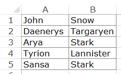
If I select cell A1 and B1 and use the Merge & Center option, it will keep the text from the left-most cell (A1 in this case) and but you will lose the data from all other cells.
Excel is not completely ruthless though – it warns you before this happens.
If you try and merge cells which have text in it, it shows a warning pop-up letting you know of this (as shown below).
If you go ahead and press OK, it will merge the two cells and keep the text from the leftmost cell only. In the above example, it will merge A1 and B1 and will show the text John only.
Merge Cells in Excel Without Losing the Data
If you don’t want to lose the text in from cells getting merged, use the CONCATENATE formula. For example, in the above case, enter the following formula in cell C1: =CONCATENATE(A1,” “,B1)
Here we are combining the cells A1 and B1 and have a space character as the separator. If you don’t want any separator, you can simply leave it out and use the formula =CONCATENATE(A1,B1).
Alternatively, you can use any other separator such as comma or semi-colon.
This result of the CONCATENATE function is in a different cell (in C1). So you may want to copy it (as values) in the cell which you wanted to merge.
You can also use the ampersand sign to combine text. For example, you can also use =A1&” “&B1
The Benefit of Not Merging Cells in Excel
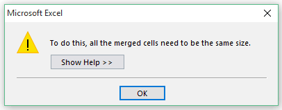
When you use Merge & Center option to merge cells, it robs you of the ability to sort that data set. If you try and sort a data set that has any merged cells, it will show you a pop-up as shown below:
Alternative to Using Merge & Center
If you want to merge cells in different columns in a single row, here is an alternative of Merge & Center – the Center Across Selection option.
Here is how to use it:
- Select the cells that you want to merge.
- Press Control + 1 to open the format cells dialogue box.
- In the Alignment tab, in the Horizontal drop-down, select Center Across Selection.
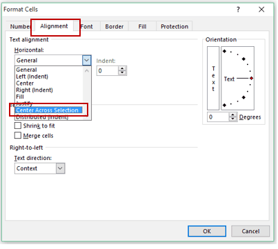
- Click OK.
This would merge the cells in a way that whatever you enter in the leftmost cell gets centered, however, you can still select each cell individually. This also does not show an error when you try and sort the data.
NOTE: For Center to Across to work, make sure only the leftmost cell has data.
You May Also Like the Following Excel Tutorials:
- How to Unmerge Cells in Excel (3 Easy Ways + Shortcut)
- CONCATENATE Excel Range (with and without separator).
- How to Find Merged Cells in Excel.
- How to Combine Cells in Excel.
- How to Combine Multiple Workbooks into One Excel Workbook.
To ensure a formatted and symmetrical look in our worksheets, we often need to merge a few cells together and center the contents of the merged cell.
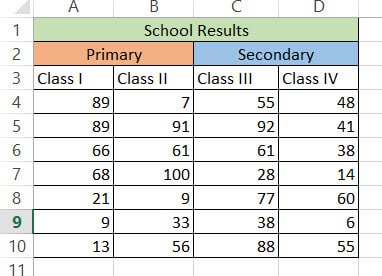
For example, you might have two columns with the same theme, like the ones shown below:
In the above image, columns A and B belong to the Primary section, while columns C and D belong to the Secondary section.
Moreover, all four columns can be grouped under the theme of ‘School Results’.
In this case, you would need to merge the headers for similar columns into one like this (colors have been added to help you see the grouping more clearly):
To bring together these similar column header cells, you might think of clicking the Merge and Center button, which makes sense.
Now, what if you select and highlight the cells you want to merge, but when you go to option to do it, you find that the Merge and Center button is grayed out?

Well, lucky for you, we have some tips that might help get you out of this problem.
In this tutorial, we will help guide you in diagnosing what is causing your Merge and Center button to be grayed out (or deactivated).
Once you’ve found the cause, we will also help you get it reactivated.
Finally, we will demonstrate some alternatives to using Merge and Center because this button is often not the best way to center contents in cells.
What does the Merge and Center Button do?
The Merge and Center button is used to merge two or more consecutive cells together into one large cell.
For example, to merge the cells A1 to D1 in the worksheet shown below, you just need to highlight the cells and click on the merge and center button.

Below is what you will see when you merge these cells

The cells now get merged into one, with the contents centered across the merged cell.
If you want to unmerge the cell back to its original contents, you can simply click on the merged cell and click on the Merge and Center button again.
Therefore, the Merge and Center button lets you do both. You can use it to merge a set of cells into one and you can use the same button to unmerge a merged cell into separate cells.
Where is the Merge and Center Button in Excel?
You will find the Merge and Center button in the ribbon under the Home tab.
If you look in the Alignment group, you will see the Merge and Center button, along with a dropdown arrow.
When you click on the arrow, you will see a number of merging options like:
- Merge and Center
- Merge Across
- Merge Cells
- Unmerge Cells
Why is Merge and Center Grayed Out? – 3 Possible Reasons
You might want to use the Merge and Center button to either merge a set of cells or unmerge an already merged set of cells.
In both cases, it can be awfully frustrating to find the button grayed out.
To solve the problem, it is important to first determine why it happened.
Here are three possible reasons your Merge and Center button might be greyed out:
The worksheet might be protected:
Worksheets or workbooks downloaded from the internet are often in Protected mode.
This is usually done to prevent users from changing, moving, or deleting information from the sheet, either accidentally or deliberately.
An Excel user can also protect a worksheet to disallow users from making selected changes to a sheet, like inserting columns, formatting rows, etc.
Putting a worksheet in protected mode usually allows the user to edit certain parts of the sheet, while most features are disabled to protect the data.
This often includes disabling the Merge and Center button too.
The workbook might be protected:
For the same reason as above, it is possible that the whole workbook itself is in Protected mode.
This could also cause the Merge and Center button to be deactivated.
The workbook might be shared:
Newer versions of Excel (from 2010 onwards) allow users to share workbooks. With the emphasis on remote collaboration, more and more people are making use of these collaboration facilities.
When you share a workbook you are allowing other users to access and make changes to your workbook concurrently.
This is great because both users are working and editing in real-time and there’s no hassle of creating multiple copies of the same workbook.
However, since Excel has to keep track of changes made by both users to a cell, it does not allow any user to merge cells while it is in shared mode.
This is done to minimize the risk of one of the cell references from disappearing
How to Find out why Merge and Center is Greyed Out
So now you know the possible reasons for your Merge and Center button to be grayed out.
It’s time to diagnose which of the three reasons is making this happen on your workbook/ worksheet.
Here’s what you need to do:
Check if the Workbook is Shared
First, check if the Merge and Center button is deactivated because your worksheet is in Protected mode.
For this, follow the steps below:
- Click on the Review tab of your Excel window
- From the ‘Changes’ group click on ‘Share Workbook’.
- This will open the ‘Share Workbook’ dialog box. Select the ‘Editing’ tab in this box.

- Right on the top portion of this window, you will see a checkbox that says ‘Allow changes by more than one user at the same time. This also allows workbook merging’. If the checkbox is checked, that means your workbook is in ‘Shared’ mode.


Check if the Worksheet is Protected
There are a number of ways to tell if your worksheet is protected. Here are the easiest two ways:
- Right-click on the sheet’s tab at the bottom of the Excel Window.
- This will make a popup menu appear.
- If one of the options in the popup menu is ‘Unprotect sheet’, it means the sheet is protected.


Here’s another giveaway:
- Click on the Review tab of your Excel window
- Look at the items under the ‘Changes’ group of this ribbon. If ‘Unprotect Sheet’ is one of the options, then the sheet is protected. If instead, you see a ‘Protect Sheet’ button, that means the sheet is not protected.


Check if the workbook is protected
- Click on the Review tab of your Excel window
- Look at the items under the ‘Changes’ group of this ribbon. If ‘Unprotect Workbook’ is one of the options, that means your workbook is protected. If instead, you see a ‘Protect Workbook’ button, it means the workbook is not protected.
- Sometimes, even if the workbook is protected, it doesn’t show as a button on the Review tab’s ribbon. In such cases, try clicking the Protect Workbook button. If it asks for a password, that means the workbook is protected.

How to Enable Merge and Center if Disabled
Once you have determined the cause of the problem, solving it is only a matter of a few clicks.
Here’s what you need to do to solve each of the above problems.
Unshare Workbook
- Click on the Review tab of your Excel window
- From the ‘Changes’ group click on ‘Share Workbook’.
- This will open the ‘Share Workbook’ dialog box. Select the ‘Editing’ tab in this box.
- Uncheck the box that says ‘Allow changes by more than one user at the same time. This also allows workbook merging’.
- Click OK to close the Share Workbook dialog box.
- You will get a prompt asking you if you are sure you want to remove the workbook from shared use. Click on Yes.
- Your book should now be free from the ‘Shared’ mode.
- Go back to the Home tab to see if the Merge and Center button is reactivated.


Did this solve the problem? If yes, then congratulations! If not, then keep reading.
Disable Protection
If the worksheet or workbook is in ‘Protected’ mode, then follow these steps:
- Click on the Review tab of your Excel window
- Look at the items under the ‘Changes’ group of this ribbon. If you see a button that says ‘Unprotect Workbook’ select it to unprotect it.
- Similarly, if you see a button that says ‘Unprotect Worksheet’ select it to unprotect it too.
- If the sheet or workbook was protected with a password, you will be asked to enter a password. Enter the password (if you know it) or find it out from the person who protected the sheet/ workbook.

- Click OK.
- Once you see the Unprotect button toggled back to ‘Protect Workbook’ or ‘Protect Worksheet’, your job is done.

- You can now go back to the Home tab to see if the Merge and Center button is reactivated.

Why it is better to Avoid using Merge and Center
You may think that Merge and Center is a good formatting tool.
After all, it helps combine multiple cells into a single large one and even centers the text across several columns (or rows).
Unfortunately, merging cells can create a number of problems for you in the long run.
You will notice that you cannot sort, filter, copy, paste or move rows and columns that have merged cells.
If you especially have a large number of merged cells in large datasets, finding out the merged cells can be quite frustrating.

As such, it is generally advised to avoid using Merge and Center as far as possible.
What you Can use Instead of Merge and Center
Due to the issues posed by cells that are merged and centered, more and more Excel experts are advising the use of the “Center across Selection” option instead.
This option gives a similar result to the Merge and Center feature, without posing problems to your spreadsheet.
To use Center Across Selection instead of Merge and Center, here’s what you need to do:
- Select the cells you want to bring together.
- Right-click on your selection.
- This will cause a popup menu to appear. Select the Format Cells option from this menu.
- The Format Cells dialog box should open now. Select the Alignment tab from this dialog box.
- Under the Text Alignment group, select the dropdown below the Horizontal menu.
- Select Center Across Selection from this dropdown.
- Click OK to close the dialog box.

Your selected cells should now look like they have been merged and centered. In essence, though, they are still separate cells.

This means you can work with them as you would work with any regular cell, minus the problems that come with Merge and Center!
Note: Center Across Selection only works horizontally, so for vertical groups of cells you may still need to merge cells.
In this tutorial, we showed you how to find out why the Merge and Center option has been grayed out for you.
We also showed what you can do once you successfully diagnose the cause of the problem.
Finally, we suggested an alternative to using Merge and Center, since this feature usually causes a number of issues when you try to edit cells and columns that they exist in.
We hope this was a helpful tutorial and that we could help you understand in-depth the issue of the Merging and Centering.
Other Excel tutorials you may like:
- How to Merge First and Last Name in Excel
- How to Split One Column into Multiple Columns in Excel
- How to Make all Cells the Same Size in Excel (AutoFit Rows/Columns)
- How to Unmerge All Cells in Excel?
- Can’t Type In Excel: 6 Possible Reasons and Solutions!
- SPILL Error in Excel – How to Fix?
- Excel Shortcuts Not Working – Possible Reasons + How to Fix?
Hello Excellers, and welcome back to another #Excel blog post in my 2021 series. Today I will show you how to achieve the same effect in Excel, without actually merging cells in Excel. Confused?. Don’t be. Do you use merged cells in your Excel worksheets?. Have you come across issues when you try to write formulas such as XLOOKUPS and VLOOKUPS. Well, those merged cells are probably causing the issues. We can use Center Across Selection as a great alternative. This method has the same visual effect, but you can ‘merge’ cells without losing any data.

So, if you want more Excel and VBA tips then sign up for my Monthly Newsletter. I share 3 Tips on the first Wednesday of the month. You will receive my free Ebook, 30 Excel Tips. Just click the link to get immediate access to my download. Keep Excelling.
Some while users love merging cells, some don’t. I admit I am the latter, in fact, I do not like them with a passion. They can be useful sometimes for example in a template or two, to make them look and flow better, but when it comes to functionality I just do not use them.
Problems With Merged Cells.
The risk I find with merging cells are
- Losing the ability to sort your data.
- Affecting the ability to copy and paste.
- You lose the ability to run VBA programming code as it just does not handle the merged well at all. Usually, more code is needed to deal with the issue.
Looks Like Merged Cells.
But, the can add to the look and feel of a spreadsheet solution. So, here is a great alternative. We do not need to compromise on the merged look. There is an alternative. Same look and feel with NO effect on functionality.
Normally a merged cell looks like the screen shot below. The cells B2 to E2 are merged.
Use Center Across Selection.
So, to get the same effect all we need to do is firstly UNMERGE the cells.
- Select the cells.
- Home Tab | Alignment Group.
- Unmerge cells.
You now have normal cell formatting.
- Select the cells that you want to appear ‘merged’. I will select B2 to E2 again.
- Home Tab | Alignment Group | Expand Alignment Settings.
- Select the Alignment Tab | Text Alignment.
- Horizontal | Center Across Selection.
- Hit ok.
Now, see that the text ‘appears’ to be centred. You can still click into the individual cells, however. This means we retain all of the worksheet functionality. Result!.
How To Excel At Excel – Formula Friday Blog Posts.
Table of contents
- Problems With Merged Cells.
- Looks Like Merged Cells.
- Use Center Across Selection.
Friends don’t let friends merge cells! This is something you hear often among Excel enthusiasts. People usually merge cells in an attempt to make a spreadsheet look nicer. That being said… not only is the beauty of a spreadsheet less important than its functionality, which is definitely adversely affected by merged cells… but there is actually a way to alter the appearance identically to merging cells without all of the many disadvantages that come with merged cells. Let’s check it out.

Exercise
If you would like to follow along with my demonstration below, here is an Exercise file: MergedCells
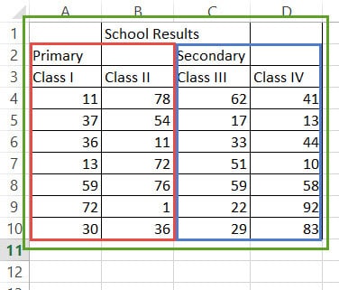
This is a fictional list of students and grades, with some merged cells at the top.
Merged Cells
The first row of data contains 3 sets of merged cells: A1 with B1; C1 with D1; and E1 with F1. If you select any of these, notice in your Alignment group that Merge and Center is selected.
Perhaps someone did this in an attempt to make their spreadsheet look less cluttered? Let’s see why this might have been a bad idea.
Why Merged Cells are Problematic
There are actually quite a few ways that merged cells can be problematic. Here are just a few.
Sort and Filter
Let’s say I would like to use the custom Filter buttons we play with in Excel Essentials. You want to filter by all students with an A.
1. Click anywhere in the top row, and on the right side of the Home tab, select Sort and Filter, and Filter.
 2. Now, Go to the dropdown created next to Grade.

Normally I would have the opportunity to filter by letter grade, but because E1 and F1 were merged cells, Excel instead only offers for you to filter by grade %. Not very helpful.
PivotTables
Maybe instead, we can make a PivotTable from the data, and pivot by the letter grade? Go to the Insert tab, and select PivotTable.

What is this? We are receiving an error because we don’t have true column labels (header row) when cells are merged like they are in our top row.. this means that Excel doesn’t know what our categories are to create a PivotTable.
(Shameless plug: come to an Excel: Pivot Tables training if you would like to learn more.)
Formulas
This is probably the biggest one for me. Let’s say I want to count the number of 22 year old students in my class. No problem! Let’s do a CountIf formula.
In I1 I entered =Countif( … then I tried to select my range, column D…. look what happens:

Excel doesn’t want to allow me to include column D alone… it wants to include Column C as well. How annoying! We could probably find our way around this formula issue, but even then, I guarantee these merged cells will get in your way with a future formula.
Macros
It is worth mentioning that there are macros that can be interfered with when you use merged cells; it depends on what type of macro you are building.
All in all, merged cells are just not worth the trouble.
Another Option: Center Across Selection
If you are truly attached to the look of merged cells, there is another option. It is called Center Across Selection.
- First, let’s undo the merged cells. Select the merged areas, then go to the Home tab, Alignment group, select the dropdown for Merge and Center, and select Unmerge cells.

2. Select A1 and B1, and Right Click on top of them. Select Format Cells.

3. In the popup screen, go to the Alignment tab, and click on the dropdown next to Horizontal. Select Center Across Selection. Click OK.

4. Repeat this step with C1 and D1 selected, then E1 and F1 selected. Appearance wise, it will look just like merged cells.

This still will be somewhat limiting; for instance, you may still have difficulty with a PivotTable unless you convert this to a Table first, but you will not experience nearly as many drawbacks as merged cells.
A Question for You
Whether you choose to center across or merge cells, I think it is an important question to ask yourself, why are you wanting to do this? Is it truly necessary? When at all possible, I would recommend avoiding either of these practices. I understand the desire to beautify a workbook, but clearly labeled columns with long lines of uninterrupted data are the truly beautiful spreadsheets. Their beauty is in their functionality; and when functionality is lost, nobody will really care much about how the top row looks. Just a thought, from someone who has “unmerged” many cells in many peoples’ spreadsheets over the years.
Thoughts?
What do you think? Has this convinced you to unmerge and never merge again? Either way, I will be here to help you.
Congratulations, Power Users!
Congratulations to our newest Power Users! For the full gallery, and more information about the WSU Microsoft Office Power User Program, please visit: wichita.edu/poweruser
Sheree Smith
(First Power User of the decade!)

There are a number of “basic errors users make in Excel” that results in their spreadsheet life being that much more challenging when it doesn’t necessarily need too. One of these, which we are discussing today, is the use (or unnecessary use) of merged cells in an Excel spreadsheet.
Why Merge Cells?
Merging cells in a spreadsheet is a process that allows you to join one or more adjacent cells (horizontally or vertically or both) into one larger cell that is then displayed across multiple columns or rows. One of the main reasons to do this is for reporting or presentation purposes – or simply put, to make a spreadsheet look nice.
If we take a quick look at the example below, you’ll see we have a simple Sales Results spreadsheet, with raw data from a number of different Departments and Divisions. A typical formatting decision for this type of information is to have the heading centred across the top of the table. To achieve this, you could merge all the heading cells to create one large cell and then centre the text. As the information in our example is raw data, we’d discourage you from doing any formatting to it at all.
The purpose of this article is not to teach you how to Merge Cells in Excel, but to provide some practical advice on some issues surrounding using merged cells unnecessarily throughout your spreadsheets.

Sample Sales Report Raw Data
IMPORTANT
- When cells are merged, the contents of only one cell (the upper-left cell) appear in the final merged cell block. The contents of all the other cells, that are being merged, are deleted.
- Excel treats the contents of the merged cell block as being contained in the top left cell of the merged block. For example, if you merged cells A1, A2, B1 and B2, Excel would contain the data in this merged block in cell A1. Important to know if you ever write a formula that involves a merged cell.
Now when it comes to creating a spreadsheet, we at ExcelSuperSite, use what we call the D.A.R.E Methodology.
This methodology breaks the design of a spreadsheet down into separate functions:
D – Data – separate your raw data and DO NOT modify its layout
A – Analysis – separate your calculations and analysis
R – Report – create separate summary/presentation sheets in your workbooks
E – Evaluate – does your information make sense
Following this methodology, merged cells won’t be used in any the Data areas nor Analysis areas of a spreadsheet, but may occasionally be used in the Reporting areas. It is generally not an issue to use merged cells in the Reporting areas of a spreadsheet as these areas are simply presenting the information obtained or analysed elsewhere and should not be used for calculation or analysis of raw data.
So What are the Issues with Merging Cells?
So let’s assume that you don’t follow our D.A.R.E. Methodology for creating your spreadsheets and that your spreadsheets are a mix of data and analysis and presentation/reporting tables. Then just for the fun of it, we also through some merged cells into the mix. Now, when trying to make changes to a spreadsheet that is constructed like this, we are faced with all sorts of complications. These include:
- Data containing merged cells can not be treated like a normal data table – meaning that we can’t use all of the tools that we might want to use for referring to a properly formatted data table, such as pivot tables, SUMIF, etc;
- Copying and pasting cell ranges is restricted to cells that are merged EXACTLY the same way as the cells being copied;
- Fill down doesn’t work if any of the cells in the range to be filled are merged;
- If you unmerge a range of cells, the merged cell contents will be placed in the top left cell of the unmerged cell range – which may not be where you want the contents to be. As a result column headings and data underneath it may now be misaligned;
- Excel won’t apply formats to a merged cell unless you select all the columns or rows that comprise the merged cell range;
- Columns with merged cells can’t be sorted;
- You can not select a single-column range if there is a merged cell in it;
- You cannot put a filter on a column with a merged cell in it;
- Formulas and Functions that refer to merged cells will not work;
The issues mentioned above can result in large amounts of additional effort when working with a spreadsheet that is not well constructed. Our advice is to only use merged cells in sheets that are purely for presentation/reporting purposes and NEVER EVER use merged cells in the Data or Analysis areas of your spreadsheets.
Our advice — only use merged cells in sheets that are purely for presentation purposes and NEVER EVER use them in the Data or Analysis areas of your spreadsheets. Click To Tweet
How Do I Achieve the Same Effect Without Merging Cells?
So how then do you achieve a similar effect without merging the underlying cells? Use the Center Across Selection cell format option.
To apply the Center Across Selection format, select the cells you want to appear merged (cells A1 through to F1 in our example) and then launch the Alignment group dialogue and click the Alignment tab. Center Across Selection is in the Horizontal: drop-down box.
Alignment Group Dialogue
The Alignment Group Dialogue box can be launched in a number of ways
- Press CTRL+1; or
- Click the small arrow in the bottom right hand corner of the Alignment Group in the Ribbon Menu – see the image below; or
- Right click on your selected cells and select “Format Cells…”

Alignment Group Dialogue

Format Cells – Center Across Selection
Using Center Across Selection will achieve a similar formatting effect on your cell selection without having to Merge cells and without any of the complications mentioned above.

Raw Data Heading Centered without Merging Cells
Continue the Discussion
So do you use merged cells in your spreadsheets? If so, do they cause any of the complications mentioned above? How do you get around these issues? Continue the discussion and add your thoughts in the comments section at the bottom of this article.
Please Share
If you liked this article or know someone who could benefit from this information, please feel free to share it with your friends and colleagues and spread the word on Facebook, Twitter and/or Linkedin.