Excel для Microsoft 365 Excel 2021 Excel 2019 Excel 2016 Excel 2013 Excel 2010 Excel 2007 Еще…Меньше
Вы можете очистить ячейки, чтобы удалить содержимое ячеек (формулы и данные), форматы (включая числовые форматы, условные форматы и границы), а также все вложенные комментарии. Очищенные ячейки остаются пустыми или неформатированные ячейки на листе.
-
Вы можете выбрать ячейки, строки или столбцы, которые нужно очистить.
Совет: Чтобы отменить выделение ячеек, щелкните любую ячейку на листе.
-
На вкладке Главная в группе Редактирование щелкните стрелку рядом с кнопкой Очистить
 и сделайте следующее:
-
Чтобы очистить все содержимое, форматы и приметки, содержащиеся в выбранных ячейках, нажмите кнопку Очистить все.
-
Чтобы очистить только форматы, примененные к выбранным ячейкам, нажмите кнопку Очистить форматы.
-
Чтобы очистить только содержимое выбранных ячеек, оставив на месте любые форматы и комментарии, нажмите кнопку Очистить содержимое.
-
Чтобы очистить примечания или заметки, прикрепленные к выбранным ячейкам, нажмите кнопку Очистить примечания и заметки.
-
Чтобы очистить все гиперссылки, прикрепленные к выбранным ячейкам, выберите очистить гиперссылки.
-
 и сделайте следующее:
Примечания:
-
Если щелкнуть ячейку и нажать кнопку DELETE или BACKSPACE, содержимое ячейки будет очищено без удаления форматов и приметок к ячейкам.
-
Если очистить ячейку с помощью окну Очистить все или Очистить содержимое,ячейка больше не содержит значения, а формула, которая ссылается на эту ячейку, получает значение 0 (ноль).
-
Если вы хотите удалить ячейки с таблицы и сдвинуть окружающие ячейки, чтобы заполнить место, вы можете выбрать ячейки и удалить их. На вкладке Главная в группе Ячейки щелкните стрелку рядом с кнопкой Удалитьи выберите удалить ячейки.
Нужна дополнительная помощь?
When working with large data sets, you may have the need to quickly delete rows based on the cell values in it (or based on a condition).
For example, consider the following examples:
- You have sales rep data and you want to delete all the records for a specific region or product.
- You want to delete all the records where the sale value is less than 100.
- You want to delete all rows where there is a blank cell.
There are multiple ways to skin this data cat in Excel.
The method you choose to delete the rows will depend on how your data is structured and what’s the cell value or condition based on which you want to delete these rows.
In this tutorial, I will show you multiple ways to delete rows in Excel based on a cell value or a condition.
Filter Rows based on Value/Condition and Then Delete it
One of the fastest ways to delete rows that contain a specific value or fulfill a given condition is to filter these. Once you have the filtered data, you can delete all these rows (while the remaining rows remain intact).
Excel filter is quite versatile and you can filter based on many criteria (such as text, numbers, dates, and colors)
Let’s see two examples where you can filter the rows and delete them.
Delete Rows that contain a specific text
Suppose you have a data set as shown below and you want to delete all the rows where the region is Mid-west (in Column B).

While in this small dataset you can choose to do delete these rows manually, often your datasets are going to be huge where deleting rows manually won’t be an option.
In that case, you can filter all the records where the region is Mid-West and then delete all these rows (while keeping the other rows intact).
Below are the steps to delete rows based on the value (all Mid-West records):
- Select any cell in the data set from which you want to delete the rows
- Click on the Data tab

- In the ‘Sort & Filter’ group, click on the Filter icon. This will apply filters to all the headers cells in the dataset

- Click on the Filter icon in the Region header cell (this is a small downward-pointing triangle icon at the top-right of the cell)

- Deselect all the other options except the Mid-West option (a quick way to do this is by clicking on the Select All option and then clicking on the Mid-West option). This will filter the dataset and only show you records for Mid-West region.

- Select all the filtered records
- Right-click on any of the selected cells and click on ‘Delete Row’

- In the dialog box that opens, click on OK. At this point, you will see no records in the dataset.

- Click the Data tab and click on the Filter icon. This will remove the filter and you will see all the records except the deleted ones.


The above steps first filter the data based on a cell value (or can be other condition such as after/before a date or greater/less than a number). Once you have the records, you simply delete these.
Some useful shortcuts to know to speed up the process:
- Control + Shift + L to apply or remove the filter
- Control + – (hold the control key and press the minus key) to delete the selected cells/rows
In the above example, I had only four distinct regions and I could manually select and deselect it from the Filter list (in steps 5 above).
In case you have a lot of categories/regions, you can type the name in the field right above the box (that has these region names), and Excel will show you only those records that match entered text (as shown below). Once you have the text based on which you want to filter, hit the Enter key.

Note that when you delete a row, anything that you may have in other cells in these rows will be lost. One way to get around this is to create a copy of the data in another worksheet and delete the rows in the copied data. Once done, copy it back in place of the original data.
Or
You can use the methods shown later in this tutorial (using the Sort method or the Find All Method)
Delete Rows Based on a Numeric Condition
Just as I used the filter method to delete all the rows that contain the text Mid-West, you can also use a number condition (or a date condition).
For example, suppose I have the below dataset and I want to delete all the rows where the sale value is less than 200.
Below are the steps to do this:
- Select any cell in the data
- Click on the Data tab
- In the ‘Sort & Filter’ group, click on the Filter icon. This will apply filters to all the headers cells in the dataset
- Click on the Filter icon in the Sales header cell (this is a small downward-pointing triangle icon at the top-right of the cell)

- Hover the cursor over the Number Filters option. This will show you all the number related filter options in Excel.
- Click on the ‘Less than’ option.

- In the ‘Custom Autofilter’ dialog box that opens, enter the value ‘200’ in the field

- Click OK. This will filter and show only those records where the sales value is less than 200
- Select all the filtered records
- Right-click on any of the cells and click on Delete Row

- In the dialog box that opens, click on OK. At this point, you will see no records in the dataset.
- Click the Data tab and click on the Filter icon. This will remove the filter and you will see all the records except the deleted ones.


There are many number filters that you can use in Excel – such as less than/greater than, equal/does not equal, between, top 10, above or below average, etc.
Note: You can use multiple filters as well. For example, you can delete all the rows where the sales value is greater than 200 but less than 500. In this case, you need to use two filter conditions. The Custom Autofilter dialog box allows having two filter criteria (AND as well as OR).
Just like the number filters, you can also filter the records based on the date. For example, if you want to remove all the records of the first quarter, you can do that by using the same steps above. When you’re working with Date filters, Excel automatically shows you relevant filters (as shown below).

While filtering is a great way to quickly delete rows based on a value or a condition, it has one drawback – it deletes the entire row. For example, in the below case, it would delete all the data which is to the right of the filtered dataset.
What if I only want to delete records from the dataset, but want to keep the remaining data intact.
You can’t do that with filtering, but you can do that with sorting.
Sort the Dataset and Then Delete the Rows
Although sorting is another way to delete rows based on value, but in most cases, you’re better off using the filter method covered above.
This sorting technique is recommended only when you want to delete the cells with the values and not the entire rows.
Suppose you have a dataset as shown below and you want to delete all the records where the region is Mid-west.
Below are the steps to do this using sorting:
- Select any cell in the data
- Click on the Data tab
- In the Sort & Filter group, click on the Sort icon.

- In the Sort dialog box that opens, select Region in the sort by column.

- In the Sort on option, make sure Cell Values is selected
- In Order option, select A to Z (or Z to A, doesn’t really matter).
- Click OK. This will give you the sorted data set as shown below (sorted by column B).

- Select all the records with the region Mid-West (all the cells in the rows, not just the region column)
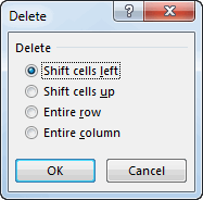
- Once selected, right-click and then click on Delete. This will open the Delete dialog box.
- Make sure the ‘Shift cells up’ option is selected.

- Click OK.


The above steps would delete all the records where the region was Mid-West, but it doesn’t delete the entire row. So, if you have any data on the right or left of your dataset, it will remain unharmed.
In the above example, I have sorted the data based on the cell value, but you can also use the same steps to sort based on numbers, dates, cell color or font color, etc.
Here is a detailed guide on how to sort data in Excel
In case you want to keep the original data set order but remove the records based on criteria, you need to have a way to sort the data back to the original one. To do this, add a column with serial numbers before sorting the data. Once you’re done with deleting the rows/records, simply sort based using this extra column you added.
Find and Select the Cells Based on Cell Value and Then Delete the Rows
Excel has a Find and Replace functionality that can be great when you want to find and select cells with a specific value.
Once you have selected these cells, you can easily delete the rows.
Suppose you have the dataset as shown below and you want to delete all the rows where the region is Mid-West.
Below are the steps to do this:
- Select the entire dataset
- Click the Home tab

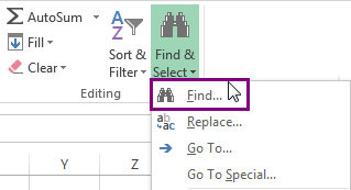
- In the Editing group, click on the ‘Find & Select’ option and then click on Find (you can also use the keyboard shortcut Control + F).

- In the Find and Replace dialog box, enter the text ‘Mid-West’ in the ‘Find what:’ field.

- Click on Find All. This will instantly show you all the instances of the text Mid-West that Excel was able to find.
- Use the keyboard shortcut Control + A to select all the cells that Excel found. You will also be able to see all the selected cells in the dataset.

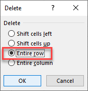
- Right-click on any of the selected cells and click on Delete. This will open the Delete dialog box.

- Select the ‘Entire row’ option
- Click OK.


The above steps would delete all the cells where the region value is Mid-west.
Note: Since Find and Replace can handle wild card characters, you can use these when finding data in Excel. For example, if you want to delete all the rows where the region is either Mid-West or South-West, you can use ‘*West‘ as the text to find in the Find and Replace dialog box. This will give you all the cells where the text ends with the word West.
Delete All Rows With a Blank Cell
In case you want to delete all the rows where there are blank cells, you can easily do this with an inbuilt functionality in Excel.
It’s the Go-To Special Cells option – which allows you to quickly select all the blank cells. And once you have selected all the blank cells, deleting these is super simple.
Suppose you have the dataset as shown below and I want to delete all the rows where I don’t have the sale value.
Below are the steps to do this:
- Select the entire dataset (A1:D16 in this case).
- Press the F5 key. This will open the ‘Go To’ dialog box (You can also get this dialog box from Home –> Editing –> Find and Select –> Go To).
- In the ‘Go To’ dialog box, click on the Special button. This will open the ‘Go To Special’ dialog box

- In the Go To Special dialog box, select ‘Blanks’.

- Click OK.


The above steps would select all the cells that are blank in the dataset.
Once you have the blank cells selected, right-click on any of the cells and click on Delete.

In the Delete dialog box, select the ‘Entire row’ option and click OK. This will delete all rows that have blank cells in it.

If you’re interested in learning more about this technique, I wrote a detailed tutorial on how to delete rows with blank cells. It includes the ‘Go To Special’ method as well as a VBA method to delete rows with blank cells.
Filter and Delete Rows Based On Cell Value (using VBA)
The last method that I am going to show you include a little bit of VBA.
You can use this method if you often need to delete rows based on a specific value in a column. You can add the VBA code once and add it your Personal Macro workbook. This way it will be available for use in all of your Excel workbooks.
This code works the same way as the Filter method covered above (except the fact that this does all the steps in the backend and save you some clicks).
Suppose you have the dataset as shown below and you want to delete all the rows where the region is Mid-West.
Below is the VBA code that will do this.
Sub DeleteRowsWithSpecificText()
'Source:https://trumpexcel.com/delete-rows-based-on-cell-value/
ActiveCell.AutoFilter Field:=2, Criteria1:="Mid-West"
ActiveSheet.AutoFilter.Range.Offset(1, 0).Rows.SpecialCells(xlCellTypeVisible).Delete
End Sub
The above code uses the VBA Autofilter method to first filter the rows based on the specified criteria (which is ‘Mid-West’), then select all the filtered rows and delete it.
Note that I have used Offset in the above code to make sure my header row is not deleted.
The above code doesn’t work if your data is in an Excel Table. The reason for this is that Excel considers an Excel Table as a list object. So if you want to delete rows that are in a Table, you need to modify the code a bit (covered later in this tutorial).
Before deleting the rows, it will show you a prompt as shown below. I find this useful as it allows me to double-check the filtered row before deleting.
Remember that when you delete rows using VBA, you can’t undo this change. So use this only when you’re sure that this works the way you want. Also, it’s a good idea to keep a backup copy of the data just in case anything goes wrong.
In case your data is in an Excel Table, use the below code to delete rows with a specific value in it:
Sub DeleteRowsinTables()
'Source:https://trumpexcel.com/delete-rows-based-on-cell-value/
Dim Tbl As ListObject
Set Tbl = ActiveSheet.ListObjects(1)
ActiveCell.AutoFilter Field:=2, Criteria1:="Mid-West"
Tbl.DataBodyRange.SpecialCells(xlCellTypeVisible).Delete
End Sub
Since VBA considers Excel Table as a List object (and not a range), I had to change the code accordingly.
Where to Put the VBA code?
This code needs to be placed in the VB Editor backend in a module.
Below are the steps that will show you how to do this:
- Open the workbook in which you want to add this code.
- Use the keyboard shortcut ALT + F11 to open the VBA Editor window.
- In this VBA Editor window, on the left, there is a ‘Project Explorer’ pane (which lists all the workbooks and worksheets objects). Right-click on any object in the workbook (in which you want this code to work), hover the cursor over ‘Insert’ and then click on ‘Module’. This will add the Module object to the Workbook and also open the Module code window on the right
- In the module window (that will appear on the right), copy and paste the above code.
Once you have the code in the VB Editor, you can run the code by using any of the below methods (make sure you have the selected any cell in the dataset on which you want to run this code):
- Select any line within the code and hit the F5 key.
- Click on the Run button in the toolbar in the VB Editor
- Assign the macro to a button or a shape and run it by clicking on it in the worksheet itself
- Add it to the Quick Access Toolbar and run the code with a single click.
You can read all about how to run the macro code in Excel in this article.
Note: Since the workbook contains a VBA macro code, you need to save it in the macro-enabled format (xlsm).
You may also like the following Excel tutorials:
- How to Delete Every Other Row in Excel
- How to Delete a Pivot Table in Excel
- How to Delete Every Other Row in Excel
- How to Move Rows and Columns in Excel (The Best and Fastest Way)
- Highlight Rows Based on a Cell Value in Excel (Conditional Formatting)
- How to Insert Multiple Rows in Excel
- Number Rows in Excel
- How to Quickly Unhide COLUMNS in Excel
- Hide Zero Values in Excel
Hello, Excellers. Welcome back to another #ExcelTip blog post in my Excel 2021 series. It is time for a neat Excel trick today in today’s #formulafriday blog post. I will demonstrate how to delete the values from your Excel cells but keep the formulas.

How To Delete Values But Keep Formulas.
One common way to set up a spreadsheet is to have input cells (which the user changes) and formula cells which work in tandem with those user input cells.
But, what if you want to delete all of the data that is in the input cells but keep your formulas intact?. Well there ( of course) is a great simple way to do it in Excel.
- Select the range of cells you want to work with or if you want to delete all non formula value cells select any cell you want.
- Home
- Editing
- Find and Select, Go to Special- which brings up the Go To Special dialog box. (Or hit F5 to use the Keyboard Shortcut).
- Select Constants- Numbers

6. Hit Ok- all of the non formula numeric cells are selected
7. Delete- to delete the values.
If you want to see all of the blog posts in the Formula Friday series you can do so by clicking on the link below.
How To Excel At Excel – Formula Friday Blog Posts.


Содержание
- How to Delete Rows if Cell Contains Specific Text in Excel
- Delete Rows With Specific Text
- Delete Rows Based on Cell Value
- Delete rows based on cell value with Find & Replace feature
- Delete Rows Based on cell value with Excel VBA Macro (VBA code)
- excel delete row if column contains value from to-remove-list
- 5 Answers 5
- New Answer 9/28/2022
- Linked
- Related
- Hot Network Questions
- Subscribe to RSS
- How to delete row based on cell value
- 7 Answers 7
- How to remove rows in Excel based on a cell value
- The fastest Excel shortcut to delete rows in your table
- Remove rows from the entire table
- Delete rows if there is data to the right of your table
- Delete rows that contain certain text in a single column
- How to remove rows in Excel by cell color
- Delete rows that contain certain text in different columns
- Excel VBA macro to delete rows or remove every other row
- You may also be interested in
How to Delete Rows if Cell Contains Specific Text in Excel
This tutorial demonstrates how to delete rows if a cell contains specific text in Excel.
Delete Rows With Specific Text
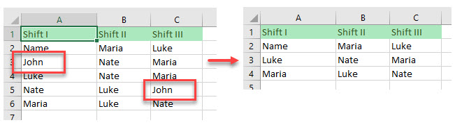
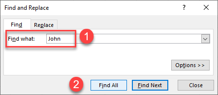
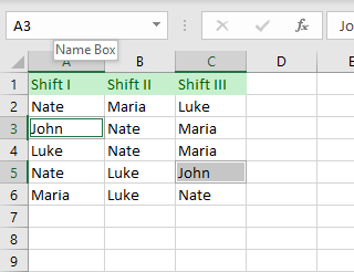
Say you have data set with names in Columns A, B, and C and want to select all cells with the name John, then delete all rows containing those cells.
- First, select the data set (A2:C6). Then in the Ribbon, go to Home > Find & Select > Find.
- The Find and Replace dialog window opens. In Find what box, type the value you are searching for (here, John), then click Find All.
You can also find and replace with VBA.
- The results are listed at the bottom of the Find and Replace window. Select all of them and click Close.
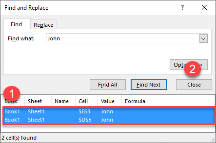
As a result, all cells with the specific value (John) are selected.
- To delete rows that contain these cells, right-click anywhere in the data range and from the drop-down menu, choose Delete.
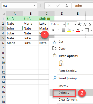
- In the Delete dialog window, choose the Entire row and click OK.
As a result, all the rows with cells that contain specific text (here, John) are deleted.
Note: You can also use VBA code to delete entire rows.
Источник
Delete Rows Based on Cell Value
This post will guide you how to use the Find & Replace feature to delete or remove all rows based on certain cell value in Microsoft Excel. Or how to delete all rows that contain certain value with VBA code in excel, such as, removing all rows if cell contains 0 or any other value.
Assuming that you have a worksheet and you want to delete rows based on cell vlaue if the value is equal to 0. In another word, if the cell value contain 0, then delete that row contain value 0. The first thing you need to do is that how to find rows that contain certain value in your worksheet. And how to solve this problem? You can use the Find & Replace command or VBA code to achieve the result.
Delete rows based on cell value with Find & Replace feature
To delete rows based on a certain cell value with Find & Replace feature, you can refer to the following steps:
1# Select the range of cells that you want to delete rows based on certain cell value.
2# on the HOME tab, click Find & Replace command under Editing group. Or just press Ctrl +F shortcut to open the Find and Replace box.
3# the Find and Replace dialog box will appear on the screen.
4# type the certain value in the Find what: text box, and then click Find All button
5# you will see that the searched result will appear in the Find and Replace window.
6# select all found values in the Find and Replace window and you will see that all cells contain certain value will be highlighted in your selected range.
7# right-click on the selected cells, and select Delete…menu from the drop-down menu list. Then choose Entire row radio button in the Delete dialog box. Click OK button.
Or you can go to HOME tab, click Delete command. Then click Delete Sheet Rows.
So far, all rows contain the certain value are deleted in your selected range. And if you want to remove the columns base on the certain value, just select Entire column radio button in the step 7.
Delete Rows Based on cell value with Excel VBA Macro (VBA code)
If you want to delete rows that contain the certain value in your worksheet with excel VBA Marco, you can refer to the following steps:
1# click on “Visual Basic” command under DEVELOPER Tab.
2# then the “Visual Basic Editor” window will appear.
3# click “Insert” ->”Module” to create a new module
4# paste the below VBA code into the code window. Then clicking “Save” button.
5# back to the current worksheet, then run the above excel macro. Click Run button.
6# select a range that you want to delete rows, click OK button. Then type a text string contained in the range of rows to delete.
Источник
excel delete row if column contains value from to-remove-list
How do I achieve that? Any help would be much appreciated.
5 Answers 5
You can flag the rows in sheet 1 where a value exists in sheet 2:
The resulting data looks like this:
You can then easily filter or sort sheet 1 and delete the rows flagged with ‘Delete’.
I’ve found a more reliable method (at least on Excel 2016 for Mac) is:
Assuming your long list is in column A, and the list of things to be removed from this is in column B, then paste this into all the rows of column C:
Then just sort the list by column C to find what you have to delete.
Here is how I would do it if working with a large number of «to remove» values that would take a long time to manually remove.
- -Put Original List in Column A -Put To Remove list in Column B -Select both columns, then «Conditional Formatting»
-Select «Hightlight Cells Rules» —> «Duplicate Values»
-The duplicates should be hightlighted in both columns
-Then select Column A and then «Sort & Filter» —> «Custom Sort»
-In the dialog box that appears, select the middle option «Sort On» and pick «Cell Color»
-Then select the next option «Sort Order» and choose «No Cell Color» «On bottom»
-All the highlighted cells should be at the top of the list. -Select all the highlighted cells by scrolling down the list, then click delete.
For a more modern answer, bring the data into powerquery, merge the 2nd sheet into the first with a left outer join. Expand. Use drop down filter to remove any rows that don’t match as null. Remove test column and file close and load back to excel
New Answer 9/28/2022
Now you can use FILTER function that simplifies it.

Note: The question requires to modify the original data sheet, this is in a general not recommended, because you are altering the input, better to have a working sheet with the transformations required.

Linked
Hot Network Questions
To subscribe to this RSS feed, copy and paste this URL into your RSS reader.
Site design / logo © 2023 Stack Exchange Inc; user contributions licensed under CC BY-SA . rev 2023.3.20.43331
By clicking “Accept all cookies”, you agree Stack Exchange can store cookies on your device and disclose information in accordance with our Cookie Policy.
Источник
How to delete row based on cell value
I have a worksheet, I need to delete rows based on cell value ..
Cells to check are in Column A ..
If cell contains «-» .. Delete Row
I can’t find a way to do this .. I open a workbook, copy all contents to another workbook, then delete entire rows and columns, but there are specific rows that has to be removed based on cell value.
UPDATE
Sample of Data I have
7 Answers 7
The easiest way to do this would be to use a filter.
You can either filter for any cells in column A that don’t have a «-» and copy / paste, or (my more preferred method) filter for all cells that do have a «-» and then select all and delete — Once you remove the filter, you’re left with what you need.
Hope this helps.
The screenshot was very helpful — the following code will do the job (assuming data is located in column A starting A1):
You could copy down a formula like the following in a new column.
. then sort on that column, highlight all the rows where the value is 1 and delete them.
if you want to delete rows based on some specific cell value. let suppose we have a file containing 10000 rows, and a fields having value of NULL. and based on that null value want to delete all those rows and records.
here are some simple tip. First open up Find Replace dialog, and on Replace tab, make all those cell containing NULL values with Blank. then press F5 and select the Blank option, now right click on the active sheet, and select delete, then option for Entire row.
it will delete all those rows based on cell value of containing word NULL.
If you’re file isn’t too big you can always sort by the column that has the — and once they’re all together just highlight and delete. Then re-sort back to what you want.
Источник
How to remove rows in Excel based on a cell value
 by Alexander Frolov, updated on March 11, 2023
This article lists several ways to delete rows in Excel based on a cell value. In this post you’ll find hotkeys as well as Excel VBA. Delete rows automatically or use the standard Find option in combination with helpful shortcuts.
Excel is a perfect tool to store data that change every now and then. However, updating your table after some changes may need really much time. The task can be as simple as removing all blank rows in Excel. Or you may need to find and delete the duplicated data. One thing we know for sure is that whenever details come or go, you search for the best solution to help you save time on the current work.
For example, you have a marketplace where different vendors sell their products. For some reason one of the vendors closed their business and now you need to delete all rows that contain the vendor’s name, even if they are in different columns.
In this post you’ll find Excel VBA and shortcuts to delete rows based on certain text or value. You’ll see how to easily find and select the necessary information before removing. If your task is not about deleting but adding rows, you can find how to do it in Fastest ways to insert multiple rows in Excel.
The fastest Excel shortcut to delete rows in your table
If you want to use the fastest method of deleting multiple rows according to the cell value they contain, you need to correctly select these rows first.
To select the rows, you can either highlight the adjacent cells with the needed values and click Shift + Space or pick the needed non-adjacent cells keeping the Ctrl key pressed.
You can also select entire lines using the row number buttons. You’ll see the number of the highlighted rows next to the last button.
After you select the necessary rows, you can quickly remove them using an Excel «delete row» shortcut. Below you’ll find how to get rid of the selected lines whether you have a standard data table, or a table that has data to the right.
Remove rows from the entire table
If you have a simple Excel list that has no additional information to the right, you can use the delete row shortcut to remove rows in 2 easy steps:
You’ll see the unused rows disappear in a snap.
Tip. You can highlight only the range that contains the values you want to remove. Then use the shortcut Ctrl + — (minus on the main keyboard) to get the standard Excel Delete dialog box allowing you to select the Entire row radio button, or any other deleting option you may need.
Delete rows if there is data to the right of your table
Ctrl + — (minus on the main keyboard) Excel shortcut is the fastest means to delete rows. However, if there is any data to the right of your main table like on the screenshot below, it may remove rows along with the details you need to keep. 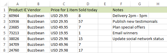
If that’s your case, you need to format your data as Excel Table first.
- Press Ctrl + T , or go to the Home tab -> Format as Table and pick the style that suites you best.
Format as Table button» title=»Go to the Home tab -> Format as Table button» width=»451″ height=»186″>
You will see the Create Table dialog box that you can use to highlight the necessary range. 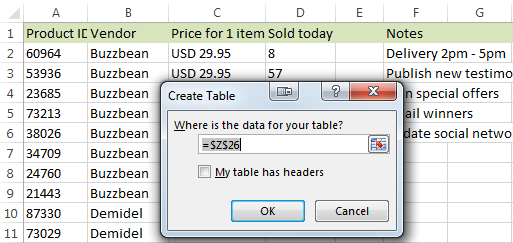
Now that your list is formatted, select the range with the values or rows you want to delete within your table. 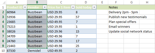
Note. Please make sure you don’t use the row buttons to select the entire rows.
Hope you’ve found this «remove row» shortcut helpful. Continue reading to find Excel VBA for deleting rows and learn how to eliminate data based on certain cell text.
Delete rows that contain certain text in a single column
If the items in the rows you want to remove appear only in one column, the following steps will guide you through the process of deleting the rows with such values.
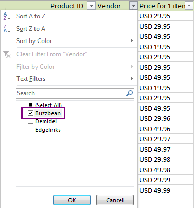
- First you need to apply Filter to your table. To do this, navigate to the Data tab in Excel and click on the Filter icon.
- Filter the column that contains the values for deleting by the needed text. Click on the arrow icon next to the column that contains the needed items. Then uncheck the Select All option and tick the checkboxes next to the correct values. If the list is long, just enter the necessary text in the Search field. Then click OK to confirm.
- Select the filtered cells in the rows you want to delete. It’s not necessary to select entire rows.
- Right-click on the highlighted range and and pick the Delete row option from the menu list.
Finally click on the Filter icon again to clear it and see that the rows with the values disappeared from your table.
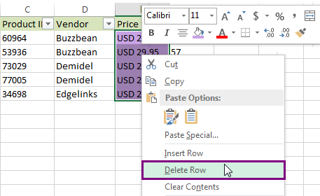
How to remove rows in Excel by cell color
The filter option allows sorting your data based on the color of cells. You can use it to delete all rows that contain certain background color.
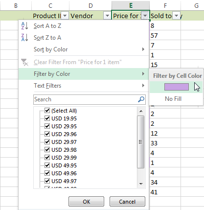
- Apply Filter to your table. Go to the Data tab in Excel and click on the Filter icon.
- Click on the small arrow next to the needed column name, go to Filter by Color and pick the correct cell color. Click OK and see all highlighted cells on top.
- Select the filtered colored cells, right-click on them and pick the Delete Row option from the menu.
That’s it! The rows with identically colored cells are removed in an instant.
Delete rows that contain certain text in different columns
If the values you want to remove are scattered around different columns, sorting may complicate the task. Below you’ll find a helpful tip to remove rows based on the cells that contain certain values or text. From my table below, I want to remove all rows that contain January which appears in 2 columns.
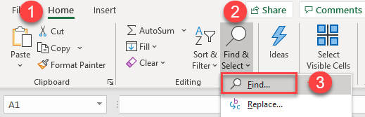
- Start by searching and selecting the cells with the needed value using the Find and Replace dialog. Click Ctrl + F to run it.
Tip. You can find the same dialog box if you go to the Home tab -> Find & Select and pick the Find option from the drop-down list.
 Find & Select and pick the Find option» title=»Go to the Home tab -> Find & Select and pick the Find option» width=»319″ height=»173″>
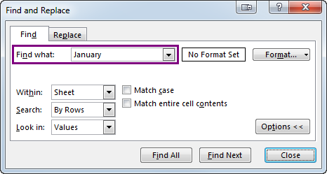
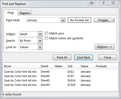
Select the found values in the window keeping the Ctrl key pressed. You will get the found values automatically highlighted in your table. 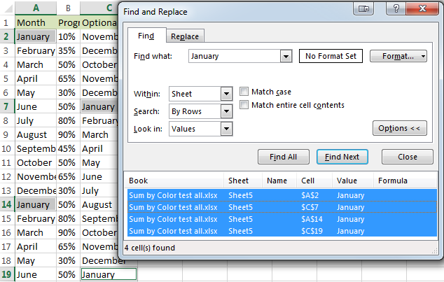
Now navigate to the Home tab -> Delete -> Delete Sheet Rows. 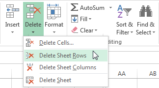 Delete -> Delete Sheet Rows» title=»Navigate to the Home tab -> Delete -> Delete Sheet Rows» width=»324″ height=»179″>
Tip. You can delete the rows with the selected values if you press Ctrl + — (minus on the main board) and select the radio button Entire rows.
Voila! The unwanted rows are deleted.
Excel VBA macro to delete rows or remove every other row
If you always search for a solution to automate this or that Excel routine, grab the macros below to streamline your delete-rows task. In this part you’ll find 2 VBA macros that will help you remove rows with the selected cells or delete every other row in Excel.
The macro RemoveRowsWithSelectedCells will eliminate all lines that contain at least one highlighted cell.
The macro RemoveEveryOtherRow as its name suggests, will help you get rid of every second/third, etc., row according to your settings. It will remove rows beginning with the current mouse cursor location and till the end of your table.
If you don’t know how to insert macros, feel free to look at How to insert and run VBA code in Excel.
Tip. If your task is to color every second/third, etc., row with a different color, you will find the steps in Alternating row color and column shading in Excel (banded rows and columns).
In this article I described how to delete rows in Excel. Now you have several useful VBA macros to delete the selected rows, you know how to remove every other row and how to use Find & Replace to help you search and select all the lines with the same values before eliminating them. Hope the tips above will simplify your work in Excel and let you get more free time for enjoying these last summer days. Be happy and excel in Excel!
You may also be interested in
Table of contents
I have a large spreadsheet, 35000 entries. One column has multiple duplicates. I would like to get rid of the rows those duplicates are in but keep one instance. How, if at all, do I find all the duplicates and keep one instance of each and then delete the rows the remaining duplicates are in? For the most part ALL of the cells in each row are the same except for a few. Example. one column lists 5 instances of RED KIDS STOCKINGS in the TITLE column with different sizes in a different cell named SIZE. I want to keep one of those rows and delete the other 4 that list RED KIDS STOCKINGS in the TITLE cell. Highlighting and clicking on each row I want to delete is very tedious with this many entries.
Hope this makes sense.
Hello!
To extract the first occurrence of a string and remove duplicate rows, you can use one of the instructions:
How to remove duplicate rows in Excel by filtering or
How to delete duplicates in Excel.
The easiest way to remove duplicates is using the Remove Duplicates tool. It is available as a part of our Ultimate Suite for Excel that you can install in a trial mode and check how it works for free.
I have VB based excel file with auto filter and formatting cells,. I want to delete old data. When I tried to put new data I got error message » 1004 application defined» Please advised me.
Hi!
When you use VBA code to select a range that is not on the active worksheet, VBA will show you a runtime error 1004.
Thanks for your reply I am totally new with VB code please help me how to delete my old data?
Can you please tell me how to delete my old data for my VB based excel file with auto filter and conditional formatting?
Hi!
I can’t see your data and your code. I’m really sorry, we cannot help you with this.
I have a spreadsheet having a specific color in column. I want to identify that cell & delete that column using VBA code. How can I do it ?
Is there a way to use a Macro to delete all rows that have a non-colored cell? I need to leave only the row not changed by the conditional formatting in one particular column. Ay help is appreciated.
I have a spreadsheet from an app that transferred all my cell # and added name, phone # address etc.
I would like to:
clean this up big time to make a mailing list.
some contacts have — home address,
Is there a way to remove the entire row if there is no address in a certain cell?
example
a first name
b second name
cell H is primary street no address no further information
I want to weed all of these people out of this excel
am I crazy for wanting this? #55&annoyed
Hello Gina Ann!
You can apply a filter to your table to display only those rows that contain empty cells in a certain column. Please see here how to create and use Excel Advanced Filter.
Then select all the rows you need to delete at once, right-click and choose the Delete option from the context menu.
I also recommend looking through carefully the «Delete rows that contain certain text in a single column» paragraph above on this page.
2016 Excel spreadsheet that has random cells with red font. Those cells are highlighted. Need to preserve the rows if they have a single cell highlighted. If the row does not have any highlighted cell, delete that row. Is that possible?
RemoveRowsWithSelectedCells — like this except RemoveRowsWithoutSelectedCell
This was awesome! saved me a lot of time! thanks!
I have a excel sheet, I have been able to filter the data and get some cells into red (to be deleted) and green (to be used) using macro. I am looking for a macro by which I can delete the complete row if a cell is red.
The red and green colors are same which we get using conditional formatting in excel 2013.
i have 300 column in sheet1,but i need only 3 column from that to sheet2.out of that 3 column i need to filter for some values and the filtered values only need to display other values are not need …that are must hide or delete.. anybody help me………………
Thank you. very helpful!
Hello,
I have a master file with data of various stores which needs to be split into various sheets store wise. I have managed to split it, but I don’t have a code to delete the blank rows in between the data.
Please look at the following video, it should help:
https://www.youtube.com/watch?v=tmA3oI0LhPg
I need to fetch data of a single coloum from a web page,but I am getting the complete page.Please tell me how do I fix it so that i will get only a single data which will update while refreshing.
For me to be able to assist you better, please send me a sample table with your data in Excel and the result you want to get. Thank you.
Copyright © 2003 – 2023 Office Data Apps sp. z o.o. All rights reserved.
Microsoft and the Office logos are trademarks or registered trademarks of Microsoft Corporation. Google Chrome is a trademark of Google LLC.
Источник
See all How-To Articles
This tutorial demonstrates how to clear the contents of multiple cells at once in Excel and Google Sheets.
Clear Cell Contents
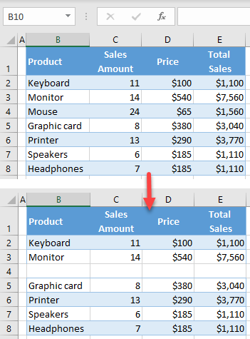
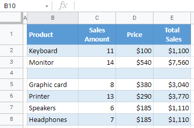
If you delete rows or columns in Excel, all cells are shifted accordingly. However, you can also delete only cells content without shifting. Say you have the following data set.
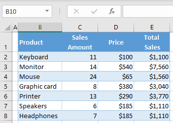
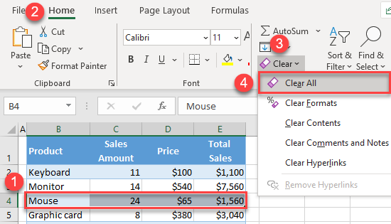
If you want to delete only values from Row 4 (range B4:E4), first select the range to clear (B4:E4). Then in the Ribbon, go to Home > Clear > Clear All (or use keyboard shortcuts).
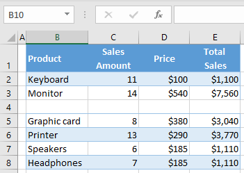
As a result, cells in Row 4 are now cleared, without shifting, so all other cells are unchanged.
Note: You can also use VBA code to clear cell contents.
Clear Contents in Google Sheets
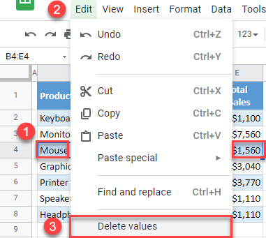
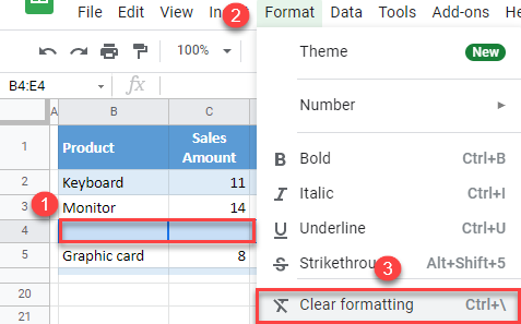
To clear cell contents without shifting in Google Sheets, follow these steps:
Select the data range you want to clear (B4:E4), and in the Menu, go to Edit > Delete values.
In this case, cell content is deleted, but the formatting remains.
To clear all formatting, select the same range (B4:E4), and in the Menu, go to Format > Clear formatting (or use the keyboard shortcut CTRL + ).
Note: This shortcut only works in Google Sheets. In Excel, CTRL + selects row differences.
Now, all content and formatting are cleared from the selected range of cells.