Excel delete all blank rows

Blank rows of data can be a big annoyance.

They’ll make certain things like navigating around our data much more difficult.

But the good news is there are lots of ways to get rid of these unwanted rows and it can be pretty easy to do it.

In this post, we’re going to take a look at 9 ways to remove blank rows from our Excel data.

Delete Blank Rows Manually

The first method is the manual way.

Don’t worry, we’ll get to the easier methods after. But if we only have a couple rows then the manual way can be quicker.

Select the blank rows we want to delete. Hold Ctrl key and click on a row to select it.

When the rows we want to delete are selected then we can right click and choose Delete from the menu.

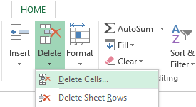
We can also delete rows using a ribbon command. Go to the Home tab ➜ click on the Delete command ➜ then choose Delete Sheet Rows.

There is also a very handy keyboard shortcut to delete rows (columns or cells). Press Ctrl + – on the keyboard.

That’s it! Our blank rows are gone now.

Delete Blank Rows Using Go To Special

Selecting and deleting rows manually is OK if we only have a couple rows to delete.

What if there are many blank rows spread across our data? Manual selection would be a pain!

Don’t worry, there is a command in Excel to select all the blank cells for us.

First, we need to select a column of our data including all the blank rows. The easiest way to do this will be to select the first cell (A1 in this example) then hold the Shift key and select the last cell (A14 in this example).

Now we can use the Go To Special command to select only the blank cells. Go to the Home tab ➜ press the Find & Select command ➜ choose Go To Special from the menu.

There’s also a handy keyboard shortcut for the Go To menu. Press Ctrl + G to open up the Go To menu then click on the Special button to open up the Go To Special menu.

Whether we open up the Go To menu then click Special or we go directly to the Go To Special menu, we will arrive at the same Go To Special menu.

Now all we need to do is select Blanks from the options and press the OK button.  This will select only the blank cells from our initial column selection.

Now we need to delete those selected rows.

1. Use any delete rows method from the Delete Blank Rows Manually section.
   • Right click ➜ Delete
   • Home tab ➜ Delete ➜ Delete Sheet Rows
   • Ctrl + – keyboard shortcut
2. In the Delete menu select Entire row and press the OK button.

Like magic, we can find and delete hundreds of blank rows in our data within a few seconds. This is especially nice when we have a lot of blank rows scattered across a long set of data.

Delete Blank Rows Using Find Command

This method is going to be very similar to the above Delete Blank Rows Using Go To Special method. The only difference is we will select our blank cells using the Find command.

Just like before, we need to select a column in our data.

Go to the Home tab ➜ press the Find & Select command ➜ choose Find from the menu.

There is also a keyboard shortcut we can use to open the Find menu. Press Ctrl + F on the keyboard.

Either way, this will open up the Find & Replace menu for us.

1. Expand the Advanced options in the Find menu.
2. Leave the Find what input box blank.
3. Select the Match entire cell contents option.
4. Search Within the Sheet.
5. Look in the Values.
6. Press the Find All button to return all the blank cells.

This will bring up a list of all the blank cells found in the selected range at the bottom of the Find menu.

We can select them all by pressing Ctrl + A. Then we can close the Find menu by pressing the Close button. Now we can delete all the blank cells like before.

Delete Blank Rows Using Filters

We can also use filters to find blank rows and delete them from our data.

First, we need to add filters to our data.

1. Select the entire range of data including the blank rows.
2. Go to the Data tab.
3. Press the Filter button in the Sort & Filter section.

We can also add filters to a range by using the Ctrl + Shift + L keyboard shortcut.

This will add sort and filter toggles to each of the column headings and we can now use these to filter out the blank.

1. Click on the filter toggle on one of the columns.
2. Use the Select All toggle to de-select all items.
3. Check the Blanks.
4. Press the OK button.

When our data is filtered, the row numbers appear in blue and filtered rows are numbers are missing.

We can now select these blank rows with the blue row numbering and delete them using any of the manual methods.

We can then press the OK button when Excel asks us if we want to Delete entire sheet row.

When we clear the filters, all our data will still be there but without the blank rows!

We can use filters in a slightly different way to get rid of the blank rows. This time we will filter out the blanks. Click on the filter toggle on one of the columns ➜ uncheck the Blanks ➜ press the OK button.

Now all our blank rows are hidden and we can copy and paste our data to a new location without all the blank rows.

Delete Blank Rows Using Advanced Filters

Similar to filter method, we can use the Advanced Filters option to get a copy of our data minus any blank rows.

To use the Advanced Filters feature, we’re going to need to do a bit of setup work.

1. We need to set up a filter criteria range. We are only going to filter based on one column, so we need one column heading from our data (in F1 in this example). Below the column heading we need our criteria (in F2 in this example), we need to enter ="" into this cell as our criteria.
2. Select the range of data to filter.
3. Go to the Data tab.
4. Select Advanced in the Sort & Filter section.

Now we need to configure the Advanced Filter menu.

1. Select Copy to another location.
2. Select the range of data to be filtered. This should already be populated if the range was selected before opening the advanced filters menu.
3. Add the criteria to the Criteria range (F1:F2 in this example).
4. Select where in the sheet to copy the filtered data.
5. Press the OK button.

We now get a copy of our data in its new location without the blanks.

Delete Blank Rows Using The Filter Function

If we are using Excel online or Excel for Office 365, then we can use one of the new dynamic array functions to filter out our blank rows.

In fact, there is a dynamic array FILTER function we can use.

FILTER Function Syntax

= FILTER ( Array, Include, [Empty] )

• Array is the range of data to filter.
• Include is a logical expression indicating what to include in the filtered results.
• Empty is the results to display if no results based on the Include argument are found.

FILTER Function To Filter Blanks

= FILTER ( CarData, CarData[Make]<>"" )

The above function needs to be entered in only one cell and the results will spill into the remaining cells as needed. The function will filter the CarData on the Make column and filter out any blanks.

It’s easy and the great part is it’s dynamic. Because our data is in an Excel table, when we add new data into the CarData table, it will appear in our filtered results.

Delete Blank Rows By Sorting

In addition to all the filtering techniques, we can sort our data to get all the blank rows.

1. Select the range of data.
2. Go to the Data tab.
3. Press the sort command. Either the ascending or descending order will work.

Now all our blank rows will appear at the bottom and we can ignore them.

If we need the original sort order of our data, we can add an index column before sorting. Then we can sort to get the blank rows at the bottom and delete them. Then we sort our data back to the original order based on the index column.

Delete Blank Rows Using Power Query

Power can easily remove blank rows in our data.

This is great is we keep getting updated data with blanks in it and need to include this in our data preparation steps.

Once our data is inside the power query editor, we can easily remove our blank data. Notice, these appear as null values inside the editor.

1. Go to the Home tab in the power query editor.
2. Press the Remove Rows button.
3. Select the Remove Blank Rows option from the menu.

= Table.SelectRows(#"Changed Type", each not List.IsEmpty(List.RemoveMatchingItems(Record.FieldValues(_), {"", null})))

This will generate the above M code using the Table.SelectRows function to select the non-null rows. This will only remove rows where the entire record has null values.

We could also get the same result by filtering out the null values in our data. Right click on any of the sort and filter toggles then uncheck the null value and press the OK button.

= Table.SelectRows(#"Changed Type", each ([Model] <> null))

Power query will again generate a step with the Table.SelectRows function, returning non-null values in a specific column.

Delete Blank Rows Using Power Automate

This one might not be as quick, easy and practical as the other methods but it can be done.

We can use Power Automate to delete blank rows in our Excel tables.

In order to do this with Power Automate, we will need to have our data in an Excel table and it will need an ID column that uniquely identifies each row.

We can set up a small Flow automation to do this.

1. We will use a manual button to trigger our flow, but we could use any number of triggers.
2. We then need to List rows present in a table to get all the rows of data from our Excel table. The best option would also be to use the Odata filters in the Show advanced options section to filter on the blank rows, but this is currently not possible to filter on blanks.
3. Because we can’t filter on the blank values with Odata filters, we need to use a Filter array data operation action to do this. We can filter on the values from the List rows present in a table action and set the condition as Make is equal to blank (leave the value empty). This will get us all the rows with blank cells.
4. We can now use the Delete a row action to delete these blank rows. We can select our ID column as the Key Column and then add the ID field from the Filter array action. This should wrap the action in an Apply to each step to delete all the blanks.

When this automation runs, it will delete any blank rows the table has.

Conclusions

Blank rows in our data can be a nuisance.

Removing them is easy and we have lots of options.

My favourite way is probably the Go To keyboard shortcut method. It’s quick, easy and does the job.

Did I miss any methods? Let me know in the comments below!

Easy Ways to Remove Blank or Empty Rows in Excel

by Avantix Learning Team | Updated April 5, 2021

Applies to: Microsoft^® Excel^® 2010, 2013, 2016, 2019, 2021 and 365 (Windows)

You can delete blank rows in Excel using several tricks and shortcuts. Check out these 5 fast ways to remove blank or empty rows in your worksheets.

In this article, we’ll focus on methods that work with all versions of Excel. In future articles, we’ll take a look at other methods available in Excel 365.

Here, we’re assuming your data is in ranges of cells with data arranged vertically below row headings or field names (and no merged cells). Excel recognizes data arranged in this way as a list or data set (or database). You can also use many of these strategies with Excel tables.

Recommended article: 15 Microsoft Excel Keyboard Shortcuts to Speed Up Formatting

Do you want to learn more about Excel? Check out our virtual classroom or live classroom Excel courses >

If you want to delete one row, you can delete the row manually:

1. Select the row. Click its heading or select a cell in the row and press Shift + spacebar.
2. Right-click the selected row heading. A drop-down menu appears.
3. Select Delete.

1. Deleting blank rows using the context menu

To delete multiple contiguous blank rows using the context menu:

1. Drag across the row headings using a mouse or select the first row heading and then Shift-click the last row heading.
2. Right-click one of the row headings. A drop-down menu appears.
3. Select Delete.

To delete multiple non-contiguous blank rows using the context menu:

1. To select non-contiguous rows, click the heading of the first row and then Ctrl-click the headings of the other rows you want to select.
2. Right-click one of the row headings. A drop-down menu appears.
3. Select Delete.

2. Deleting blank rows using a keyboard shortcut

To delete multiple contiguous blank rows using a keyboard shortcut:

1. Drag across the row headings using a mouse or select the first row heading and then Shift-click the last row heading.
2. Press Ctrl + – (minus sign at the top right of the keyboard) to delete the selected rows.

To delete multiple non-contiguous blank rows using a keyboard shortcut:

1. To select non-contiguous rows, click the heading of the first row and then Ctrl-click the headings of the other rows you want to select.
2. Press Ctrl + – (minus sign at the top right of the keyboard) to delete the selected rows.

3. Deleting blank rows by sorting

An easy way to delete blank rows is to sort the data so that blanks appear at the bottom and you can then ignore them.

To delete blank rows by sorting:

1. Select the entire range of data (not just the column you want to sort).
2. Click the Data tab in the Ribbon.
3. Select Sort in the Sort & Filter group. A dialog box appears. Assuming you have a header row, select My data has headers.
4. Beside Sort by, select the field or column with the blanks you want to remove and then select the appropriate sorting option (such as A-Z, smallest to largest, ascending or descending) to display blanks at the bottom of the data set.
5. Click OK. Blank rows will now appear at the bottom of the data set and can be ignored.

Below is the Sort dialog box:

4. Deleting blank rows using Go to Special to highlight blanks

A great way to remove blank rows in a range of data is to use Go to Special.

The Go To Special dialog box displays the following options:

To find and remove blank rows using Go to Special:

1. Select one column where there are blank cells in the column (we’re assuming here that the rest of the row is blank). If there is sensitive data above or below the list that you don’t want to delete, select the cells in the column from the first cell in the range to the last cell in the range (you could click in the first cell and Shift-click in the last cell).
2. Press Ctrl + G. The Go To dialog box appears.
3. Click Special to display the Go To Special dialog box. Alternatively, you can click the Home tab in the Ribbon and then select Go To Special from the Find & Select drop-down menu.
4. Select Blanks in the Go to Special dialog box and click OK. Excel will select all of the blank cells within the selected range.
5. Right-click one of the selected blank cells and select Delete. A dialog box appears.
6. Select Entire Row.
7. Click OK.

The Delete dialog box appears as follows:

Although you can also use the Find command to find blanks, it’s much easier to use Go to Special.

5. Deleting blank rows using filtering

You can also delete blank rows using filtering (traditionally called AutoFiltering).

To delete blank rows using Filter:

1. Select the range of cells that includes all of the data in the data set (including blank rows).
2. Click the Data tab in the Ribbon.
3. Select Filter in the Sort & Filter group. Alternatively, you can press Ctrl + Shift + L. Arrows appear beside the field names.
4. Click the arrow beside the field name with the blank cells in  rows you want to delete.
5. Turn off or de-select Select All.
6. Select Blanks. You will likely need to scroll down to select Blanks.
7. Select the row headings of the filtered rows by clicking the first row heading and Shift-clicking the last row heading.
8. Right-click one of the selected headings. A drop-down menu appears.
9. Select Delete Row.
10. Click the Data tab in the Ribbon and select Clear in the Sort & Filter group to remove the filtering.

In the example below, the Promotion field is filtered to display blanks:

You will now be able to sort, filter and create pivot tables with the list.

Subscribe to get more articles like this one

Did you find this article helpful? If you would like to receive new articles, JOIN our email list.

More resources

How to Use Flash Fill in Excel (4 Ways with Shortcuts)

How to Lock Cells in Excel (Protect Formulas and Data)

3 Excel Strikethrough Shortcuts to Cross Out Text or Values in Cells

Use Conditional Formatting in Excel to Highlight Dates Before Today (3 Ways)

How to Replace Blank Cells in Excel with Zeros (0), Dashes (-) or Other Values

Related courses

Microsoft Excel: Intermediate / Advanced

Microsoft Excel: Data Analysis with Functions, Dashboards and What-If Analysis Tools

Microsoft Excel: Introduction to Power Query to Get and Transform Data

Microsoft Excel: New and Essential Features and Functions in Excel 365

Microsoft Excel: Introduction to Visual Basic for Applications (VBA)

VIEW MORE COURSES >

Our instructor-led courses are delivered in virtual classroom format or at our downtown Toronto location at 18 King Street East, Suite 1400, Toronto, Ontario, Canada (some in-person classroom courses may also be delivered at an alternate downtown Toronto location). Contact us at info@avantixlearning.ca if you’d like to arrange custom instructor-led virtual classroom or onsite training on a date that’s convenient for you.

Copyright 2023 Avantix^® Learning

Microsoft, the Microsoft logo, Microsoft Office and related Microsoft applications and logos are registered trademarks of Microsoft Corporation in Canada, US and other countries. All other trademarks are the property of the registered owners.

Avantix Learning |18 King Street East, Suite 1400, Toronto, Ontario, Canada M5C 1C4 | Contact us at info@avantixlearning.ca

How To Delete Blank Rows In Excel: Step-by-Step (2023)

How To Delete Blank Rows In Excel: Step-by-Step (2023)

Everyone hates empty rows in their data.

Fortunately, there are 2 ways to remove all the blank rows in your spreadsheet – in just a few clicks.

Which method fits you best comes down to this really important distinction:

1) “I want to delete rows that contain 1 or more blank cells”

2) “I want to delete rows if they only contain blank cells”

Let’s dive in🤿

Oh, and click here to download the Excel file I’m using in this guide.

How to delete blank rows if 1 or more cells are blank

This method deletes rows in your data if they contain 1 or more blank cells.

That means rows like the 3 ones shown in the screenshot would be considered as blanks, and then removed.

If that’s the kind of empty rows you want to remove, follow these steps:

1. In the Home tab, click the ‘Find & Select’ button on the right side of the Ribbon, so you can start to find blank rows.

2. Select ‘Go To Special’.

3. Select Blanks and click OK.

This select only the blank cells in your data.

Now, you need to delete entire rows instead of just the selected cells.

4. From the Home tab, click the arrow below the Delete button and choose ‘Delete Sheet Rows’.

And that’s how to delete blank rows in Excel.

Well…

If blank rows = rows that contain 1 or more blank cells⚠️

This is quite important, as you can accidentally remove empty rows that shouldn’t have been removed if you just blindly use this method.

If you mean blank rows must be completely empty before they should be deleted, use the method below instead.

PRO TIP: Shortcuts

You can use these shortcuts to open the ‘Go To Special’ dialog box instead of the method above:

• Press F5 (for Windows and Mac)
• Press Ctrl + G and click the ‘Special’ button (for Windows and Mac)

And continue with the remaining steps from above to remove blank rows.

How to delete blank rows if all cells are blank

This is what I’d call the proper way to remove blank rows. Although it’s a bit more cumbersome.

It’s more restrictive, meaning that it generally will remove less rows than the method above✂️

This way, a row will only be considered to be blank there are only empty cells in the entire row (within the columns of the data set).

In the screenshot, only 1 row is completely blank, while the other 3 highlighted rows are partially blank.

Now, to remove completely blank rows with this method, follow these steps:

1. Select the relevant columns (A, B, and C).

Make sure you select the entire columns. If you don’t, you won’t filter the entire dataset and you won’t be successful when you remove blank rows in a few seconds.

2. Go to the Data tab and click the Filter button.

And you can see the filter buttons next to each of the column headers.

3. Click the first filter button and make sure there’s only a checkmark in the Blanks checkbox.

You do that by unchecking the ‘Select All’ option before putting the checkmark in Blanks.

Now, only rows that have empty cells in column A are visible.

If you used method 1, row 2 would be considered a blank row and would be deleted🤔

4. Repeat step 3 for all other columns in the data set.

In this case, it’s only column B and C.

So, for each data column, go into the filter, uncheck ‘Select all’ and make sure there’s a checkmark in Blanks.

This leaves only the real empty rows.

5. Select all the blank rows.

6. Click the drop-down arrow below the ‘Delete’ button in the Home tab, and select ‘Delete Sheet Rows’.

And that’s how to remove blank rows in Excel -> the proper way.

7. Remove the filter by clicking the Filter button.

And your blank rows are gone!

Keep in mind the rows partially empty rows are still visible.

Pretty cool, huh?😎

Video guide: Delete blank rows

Want to watch how to remove blank rows on video instead of reading?

Then see my Youtube video and learn everything you need to know about this proper way to delete blank rows.

Delete blank rows individually

If you need to get rid of a small number of blank rows, you can do it manually – one blank row at a time.

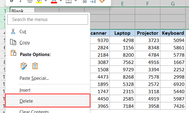
Just right-click on the single row number for the row you want to delete.

And select Delete.

Then it’s gone!

Pretty easy right?

That way, you can assess whether the row is to be considered a blank row or not.

Obviously, this method takes way too long in big spreadsheets⏳

That’s it – Now what?

That’s how to delete blank rows in Excel.

Both ways are fine for deleting blank rows. One is quick and one is thorough.

But be aware that with the quick method (first method), you might remove blank rows that shouldn’t be deleted.

So, while the quick for deleting blank rows works in some scenarios, I definitely recommend learning the “hard” way.

The reason why you’re deleting blank rows in the first place is to ensure there are no gaps in your data.

This helps with calculations!

But you know what also helps with calculations?

Learning the absolute best functions Microsoft Excel has to offer.

Click here to read more about my free training that teaches you IF, SUMIF, VLOOKUP, and pivot tables.

It’ll make you an Excel wizard in just 30 minutes.

Kasper Langmann2023-01-19T12:25:51+00:00

When importing and copying tables in Excel, empty strings and cells can be formed. They always district and interfere with the work.

Some formulas may not work correctly. It is impossible to use a number of tools for an incompletely filled range. We will learn how to quickly delete empty cells at the end or middle of a table. We will use simple tools available to the user of any level.



How to remove empty rows in the Excel table?

To show you how to delete extra lines, to illustrate the order of actions, take a table with conditional data:

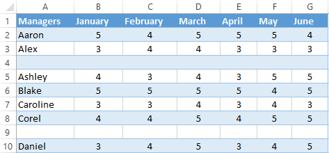
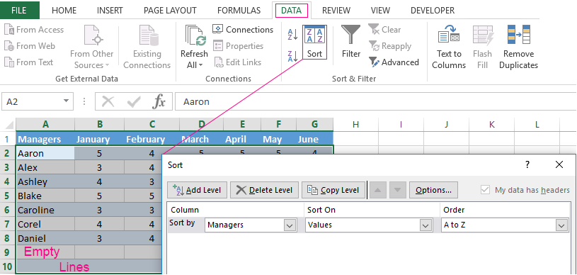
Example 1: Sorting data in a table. Select the entire table. Open the «DATA» tab — «Sort and Filter» tool — press the «Sort» button. Another way is to right-click on the selected range and do the sorting «A to Z».

Empty rows after sorting in ascending order are at the bottom of the range.

If the order of the values is important, then before the sorting, you need to insert an empty column, make a through numbering. After sorting and deleting blank lines, sort the data by the inserted column with the numbering again.

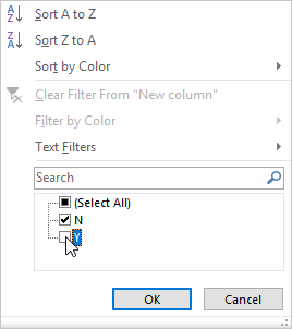
Example 2: Filter. The range must be formatted as a table with headers. We select the «cap». On the «DATA» tab, we click the «Filter» button («Sort and Filter»). A down arrow appears to the right of each column name. Push — opens the filtering window. Remove the selection in front of the name «Empty».

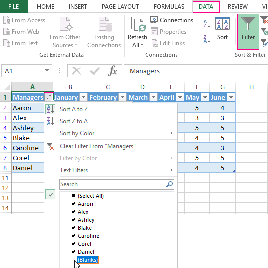
You can delete empty cells in the Excel line the same way. Select the required column and filter its data.

Example 3: Selecting a group of cells. Select the entire table. In the main menu on the «Edit» tab we click the button «Find and Select». Select the «Go To Special» tool. In the window that opens, select the «Blanks».

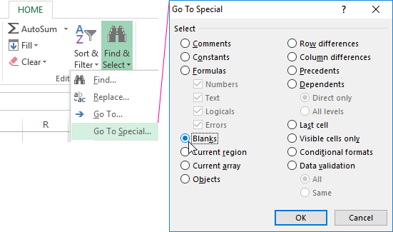
The program marks empty cells. On the main page we find the «HOME»-«Delete»-«Delete Cells».

The result is a filled range of «no voids».

Attention! After the removal, some of the cells jump upwards — the data can be messed up. Therefore, for the overlapping ranges, the instrument is not suitable.

Helpful advice! The shortcut to delete the selected row in Excel is CTRL + «-«. And for its selection, you can press the hotkey combination SHIFT + SPACEBAR.



How to remove repeated rows in Excel?

To remove the same rows in Excel, select the entire table. Go to the tab «DATA»-«Data Tool»-«Delete Duplicates».

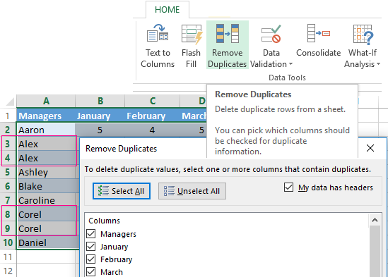
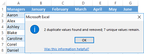
In the window that opens, select those columns that contain duplicate values. Since you need to delete duplicate rows, all columns should be highlighted. After clicking OK Excel creates a mini-report of the form:

How to remove each second line in Excel?

You can use the macro to break the table. For example, this:

Sub Delete_Every_Other_Row()
' Dimension variables.
Y = False ' Change this to True if you want to
' delete rows 1, 3, 5, and so on.
I = 1
Set xRng = Selection
' Loop once for every row in the selection.
For xCounter = 1 To xRng.Rows.Count
' If Y is True, then...
If Y = True Then
' ...delete an entire row of cells.
xRng.Cells(I).EntireRow.Delete
' Otherwise...
Else
' ...increment I by one so we can cycle through range.
I = I + 1
End If
' If Y is True, make it False; if Y is False, make it True.
Y = Not Y
Next xCounter
End Sub


And you can do it by hand. We offer a simple way, accessible to each user.

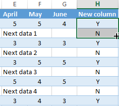
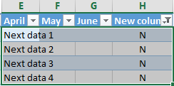
1. At the end of the table, make an auxiliary column. Fill with alternate data. For example, «N Y N Y», etc. We enter values in the first four cells. Then select them. «We catch» for the black cross in the lower right corner and copy the letters to the end of the range.



2. Install the «Filter». Filter the last column by the value of «Y».



3. Select all that is left after filtering and delete.



4. We remove the filter — only cells with «N» will remain.

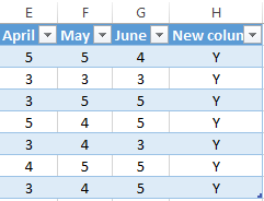
The auxiliary column can be eliminated and operated with a «decimated table».

How to delete hidden rows in Excel?

When the user had hidden some information in the rows he was not distracted from his work. I thought that later the data would be needed. It is not needed — hidden rows can be deleted: they affect the formulas, interfere.

In the training table are hidden rows 5, 6, 7:

We will remove them.

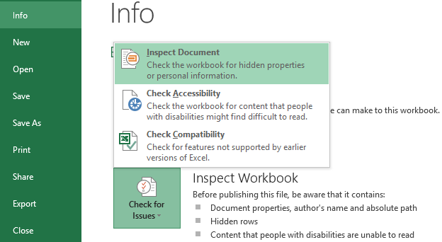
1. Go to «FILE»-«Info»-«Check for Issues» the tool «Inspect Document».



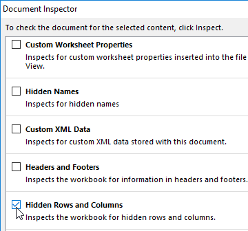
2. In the opened window, put a tick in front of the «Hidden Rows and Columns». Click «Inspect».



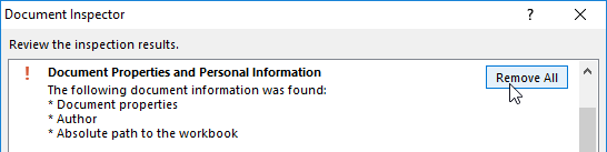
3. After a few seconds, the program displays the result of the test.



4. Click «Remove All». A corresponding notification will appear on the screen.

As a result of the work done, the hidden cells are deleted, the numbering is restored.

Thus, remove the empty, repeating or hidden cells of the table using the built-in functionality of the Excel program.

While working with large datasets in Excel, you may need to clean the data to use it further.

One common data cleaning step is to delete blank rows from your data in Excel.

In this tutorial, I will show you how to remove blank rows in Excel using different methods.

While there is no in-built feature in Excel to do this, it can quickly be done using simple formula techniques or using features such as Power Query or Go-To Special.

And for VBA aficionados, I’ll also give you a simple VBA code that you can use to quickly remove all blank rows from your data set in Excel.

Delete Blank Rows Using the SORT Functionality

One of the easiest ways to quickly remove blank rows is by sorting your data set so that all the blank rows are stacked together.

Once all the empty rows are together, you can manually select and delete them in one go.

However, you cannot simply apply the sorting on your existing dataset (as it can alter your data set by rearranging the rows while sorting). We will need to add a helper column which we will use to sort the data and then delete the blank rows.

Let me show you how it works using a simple example.

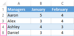
Below I have a data set where I have some blank rows that I want to remove from this data set:

Here are the steps to remove the blank columns using a helper column and sort functionality:

1. We first need to insert a helper column to the left of the data set. To do this, select the column header of the first column, right click and then click on insert

1. Now enter the below formula in cell A1, and then copy this for all the cells in the column

=IF(COUNTA(B1:XFD1)=0,"Blank","Not Blank")

This above formula would give us the result “Blank” when the row is empty and the result “Not Blank” when the row is not empty.

1. Select the entire dataset (including the helper column)
2. Click the Data tab

1. Click on the Sort icon (in the Sort & Filter group)

1. In the Sort dialog box that opens, unchecked the option ‘My data has Headers’

1. Open the Sort By drop-down and select Column A (which is our helper column)

1. Keep the ‘Sort On’ and ‘Order’ values as is
2. Click OK

The above steps would sort your data set so that all the blank rows are stacked up together at the top, and the remaining data set is below the blank rows.

1. Select all the blank rows, right click and delete

1. Once done, feel free to remove the helper column

Note: When we sort our data set using the steps above, it will not mess with the original order of the rows. It will only bring all the blank rows at the top while keeping your original data set intact.

For this method to work, every cell in the blank row needs to be actually blank. If it has a space character or null string, it would not be considered blank.

Delete Blank Rows Using Find and Replace

Another smart way to quickly delete blank rows from your data set is by using the Find and Replace functionality.

Let me show you how it works with an example.

Below have a data set where I have some blank crows that I want to delete:

Here are the steps to do this using a helper column with Find and Replace functionality:

1. The first step is to add a helper column to our dataset. To do this, select the column header of the first column, right-click, and then click on insert. This will insert a blank column to the left of the data set

1. Now enter the below formula in cell A1, and then copy this for all the cells in the column

=IF(COUNTA(B1:XFD1)=0,"Blank","Not Blank")

This above formula would give us the result “Blank” when the row is empty and the result “Not Blank” when the row is not empty.

1. Select the helper column (not the entire dataset).
2. Hold the Control key and press the F key. This will open the Find and Replace dialog box. You can also do this by clicking the Home tab, clicking on the Find & Replace icon in the Editing group, and then clicking on the Find option.
3. In the Find and Replace dialog box, enter ‘Blank’ in the Find what field

1. Check the option – Match entire cell contents

1. In the Look in drop-down, select Values.

1. Click on the Find all button.

1. This will find all the cells that have the value blank in them and show the list below the find and replace dialog box.

1. Hold the Control key and Press the A key once. This will select all the cells that have been found by the Find and Replace option.

1. Right-click on any of the selected cells and then click the Delete option.

1. In the Delete dialog box that opens up, select the Entire row option

1. Click OK. This should remove all the blank rows from your data set
2. Once done, feel free to remove the helper column.

For this method to work, every cell in the blank row needs to be actually blank. If it has a space character or null string, it would not be considered blank.

Also read: Delete Blank Columns in Excel (3 Easy Ways + VBA)

Delete Blank Rows Using Go To Special (Use with Caution)

Let me also show you how to remove blank rows in Excel by using the Go-to special technique.

However, let me warn you that there is a possibility that this may end up deleting some of the rows that may not be completely blank (and may only have a few cells that are blank).

I recommend you do not use this method with large data sets.

Below I have a data set where I have some blank rows that I want to remove:

Here are the steps to do this using the Go To Special technique:

1. Select the entire data set
2. Press F5 on your keyboard to open the Go To dialog box.

1. Click on the Special button. This will open the Go To Special Dialog box. Alternatively, you can click the Home tab, then click the Find & Replace icon in the Editing group, and then click the ‘Go To Special’ option.

1. In the Go To Special dialog box that opens up, click on the Blank option

1. Click OK.

The above steps would select all the cells that are blank in the data set. Since all the cells in a blank row would be empty, this would end up selecting all the blank rows.

1. Right-click on any of the selected blank cells and click on the Delete option

1. In the Delete dialog box that opens, select the Entire row option

1. Click OK

The above steps would remove all the rows that contain blank cells.

CAUTION: This method should only be used if you are sure that there are no blank cells in your data set except the ones that are in the blank rows. In case there are blank cells in an otherwise non-blank row, even these rows would be deleted, as this method works by selecting the blank cells and then deleting the entire row of that blank cell.

Remove Blank Rows Using VBA Macro

If you need to delete blank rows often, you can also consider using a simple VBA macro code to do this.

Even if you are an absolute beginner with Excel VBA macros, don’t worry. I will show you how to set it up properly so that you can use it again and again.

But let me first give you the VBA code.

Below is the VBA code that will go through your entire data set and delete all the blank rows:

'Code Developed by Sumit Bansal from https://TrumpExcel.com

Sub DeleteBlankRows()

Dim EntireRow As Range
On Error Resume Next
MsgBox Selection.Row.Count

Application.ScreenUpdating = False

        For i = Selection.Rows.Count To 1 Step -1
            Set EntireRow = Selection.Cells(i, 1).EntireRow
            If Application.WorksheetFunction.CountA(EntireRow) = 0 Then
                EntireRow.Delete
            End If
        Next

Application.ScreenUpdating = True

End Sub

The above VBA code uses a simple For Next loop to go through each row in your data set and check whether the row is empty or not using the COUNTA function.

As soon as it finds an empty row, it deletes it and moves to the next one.

Now let me show you the steps on how to set up this VBA code to use it in Excel:

1. Select the dataset that has the blank rows that you want to remove
2. Click the Developer tab in the ribbon. If you do not see the developer tab, click here to find out how to get it.
3. Click on the Visual Basic option. This will open the VB editor, where we are going to add the VBA code that I’ve given above.

Excel Tip: You can also use the keyboard shortcut ALT + F11 to open the VB editor

1. In the VB editor, click on the Insert option in the menu.

1. Click on the module option. This will insert a new module and open the module code window.

1. Copy and paste the VBA code I’ve given above in the module code window.

1. Place your cursor anywhere within the code and click on the Run Sub/Userform icon in the toolbar (or press the F5 key)

1. Close the VB Editor

The above steps would remove all the blank rows from your data set.

Here are a few things you need to know when using this macro in Excel:

• Once you have added the VBA code to your Excel file, you need to save your Excel file as a Macro-enabled file (with a .XLSM extension)
• If you follow the steps above to insert a module and then add this code to the module, it is only going to work in the workbook where it has been added.
• If you want this code to work on all your Excel workbooks, you should save this in your personal macro workbook. Once the code has been saved in the Personal Macro Workbook, you can use it in any Excel workbook on your system.

Note: Remember that any changes done through a VBA code are irreversible, and you will not be able to get your original data back after you have run the macro code. So it’s always a good idea to make a backup copy of your data just in case you need it in the future.

Delete Blank Rows Using Power Query (Get & Transform)

Another really quick way to remove blank rows from a dataset Excel is by using Power Query.

With Power Query, you can open your data set in the Power Query Editor and delete all the blank rows with a few clicks. When you have the desired result in the Power Query Editor, you can quickly get this data back in Excel as a new table.

Let me show you how it works.

Below I have the same data set where I have some blank rows that I want to remove.

Here are the steps to delete blank rows using Power Query:

1. The first step would be to convert your data into an Excel table (if it’s not in the Excel table format already). To do this, select the dataset, then click on the Insert tab in the ribbon, and then click on the Table icon. Or you can use the keyboard shortcut Control + T

1. In the Create Table dialog box, make sure that the range is correct and the ‘My Table has headers’ option is checked.

1. Click Ok. Doing this would convert our dataset into an Excel Table that we can use in Power Query.
2. Select any cell in the Excel Table
3. Click the Data tab
4. In the Get & Transform Data group, click on the From Table/Range option. This will open the Power Query Editor.

1. In the Table that shows in the Power Query Editor, click on the first column filter icon.

1. Click on Remove Empty. This will remove all the blank cells from the data set.

1. Click on the Close & Load option in the ribbon.

The above steps would insert a new worksheet in your workbook where the resulting table would be inserted.

One huge benefit of using Power Query is that when you have set the process once, you can reuse this query again and again.

For example, in case you change your original data set, or add more rows to your data set, then you do not need to repeat the same steps. you can simply go to the resulting table you got after step 9, right-click on any of the cells and then click on Refresh.

When you refresh the query, it repeats the same steps in the back end, where it goes back to the original table, checks the data, removes the blank rows, and updates the resulting table in a few seconds.

In this tutorial, I showed you five different ways to delete blank rows from your data set in Excel.

The easiest would be to use a helper column and then and then either use the sort functionality to stack all the blank rows together and delete them, or use Find and Replace to find all the blank rows and delete them manually.

Another easy and popular way to remove blank rows is by using the Go To Special technique. However, you should use it cautiously as it can also end up deleting those rows that are not completely empty.

If you’re comfortable using VBA, you can also use a simple macro code I have given in this article to quickly all the blank rows.

And finally, I have also covered how to do this using Power Query.

Other Excel articles you may also like:

• How to Delete Alternate Rows in Excel
• Delete Blank Columns in Excel
• The Ultimate Guide to Find and Remove Duplicates in Excel.
• Remove Spaces in Excel – Leading, Trailing, and Double.
• How to Insert Multiple Rows in Excel.
• Insert a Blank Row after Every Row in Excel (or Every Nth Row)
• 7 Quick & Easy Ways to Number Rows in Excel.
• Useful Excel Macro Examples.
• Delete rows based on cell value in Excel