Use the DATEDIF function when you want to calculate the difference between two dates. First put a start date in a cell, and an end date in another. Then type a formula like one of the following.
Warning: If the Start_date is greater than the End_date, the result will be #NUM!.
Difference in days
In this example, the start date is in cell D9, and the end date is in E9. The formula is in F9. The “d” returns the number of full days between the two dates.
Difference in weeks
In this example, the start date is in cell D13, and the end date is in E13. The “d” returns the number of days. But notice the /7 at the end. That divides the number of days by 7, since there are 7 days in a week. Note that this result also needs to be formatted as a number. Press CTRL + 1. Then click Number > Decimal places: 2.
Difference in months
In this example, the start date is in cell D5, and the end date is in E5. In the formula, the “m” returns the number of full months between the two days.
Difference in years
In this example, the start date is in cell D2, and the end date is in E2. The “y” returns the number of full years between the two days.
Calculate age in accumulated years, months, and days
You can also calculate age or someone’s time of service. The result can be something like “2 years, 4 months, 5 days.”
1. Use DATEDIF to find the total years.
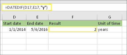
In this example, the start date is in cell D17, and the end date is in E17. In the formula, the “y” returns the number of full years between the two days.
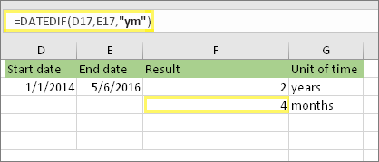
2. Use DATEDIF again with “ym” to find months.
In another cell, use the DATEDIF formula with the “ym” parameter. The “ym” returns the number of remaining months past the last full year.
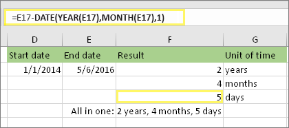
3. Use a different formula to find days.
Now we need to find the number of remaining days. We’ll do this by writing a different kind of formula, shown above. This formula subtracts the first day of the ending month (5/1/2016) from the original end date in cell E17 (5/6/2016). Here’s how it does this: First the DATE function creates the date, 5/1/2016. It creates it using the year in cell E17, and the month in cell E17. Then the 1 represents the first day of that month. The result for the DATE function is 5/1/2016. Then, we subtract that from the original end date in cell E17, which is 5/6/2016. 5/6/2016 minus 5/1/2016 is 5 days.
Warning: We don’t recommend using the DATEDIF «md» argument because it may calculate inaccurate results.
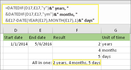
4. Optional: Combine three formulas in one.
You can put all three calculations in one cell like this example. Use ampersands, quotes, and text. It’s a longer formula to type, but at least it’s all in one. Tip: Press ALT+ENTER to put line breaks in your formula. This makes it easier to read. Also, press CTRL+SHIFT+U if you can’t see the whole formula.
Download our examples
Other date and time calculations
As you saw above, the DATEDIF function calculates the difference between a start date and an end date. However, instead of typing specific dates, you can also use the TODAY() function inside the formula. When you use the TODAY() function, Excel uses your computer’s current date for the date. Keep in mind this will change when the file is opened again on a future day.
Please note that at the time of this writing, the day was October 6, 2016.
Use the NETWORKDAYS.INTL function when you want to calculate the number of workdays between two dates. You can also have it exclude weekends and holidays too.
Before you begin: Decide if you want to exclude holiday dates. If you do, type a list of holiday dates in a separate area or sheet. Put each holiday date in its own cell. Then select those cells, select Formulas > Define Name. Name the range MyHolidays, and click OK. Then create the formula using the steps below.
1. Type a start date and an end date.
In this example, the start date is in cell D53 and the end date is in cell E53.
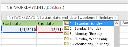
2. In another cell, type a formula like this:
Type a formula like the above example. The 1 in the formula establishes Saturdays and Sundays as weekend days, and excludes them from the total.
Note: Excel 2007 doesn’t have the NETWORKDAYS.INTL function. However, it does have NETWORKDAYS. The above example would be like this in Excel 2007: =NETWORKDAYS(D53,E53). You don’t specify the 1 because NETWORKDAYS assumes the weekend is on Saturday and Sunday.
3. If necessary, change the 1.
If Saturday and Sunday are not your weekend days, then change the 1 to another number from the IntelliSense list. For example, 2 establishes Sundays and Mondays as weekend days.
If you are using Excel 2007, skip this step. Excel 2007’s NETWORKDAYS function always assumes the weekend is on Saturday and Sunday.
4. Type the holiday range name.
If you created a holiday range name in the “Before you begin” section above, then type it at the end like this. If you don’t have holidays, you can leave the comma and MyHolidays out. If you are using Excel 2007, the above example would be this instead: =NETWORKDAYS(D53,E53,MyHolidays).
Tip: If you don’t want to reference a holiday range name, you can also type a range instead, like D35:E:39. Or, you could type each holiday inside the formula. For example if your holidays were on January 1 and 2 of 2016, you’d type them like this: =NETWORKDAYS.INTL(D53,E53,1,{«1/1/2016″,»1/2/2016»}). In Excel 2007, it would look like this: =NETWORKDAYS(D53,E53,{«1/1/2016″,»1/2/2016»})
You can calculate elapsed time by subtracting one time from another. First put a start time in a cell, and an end time in another. Make sure to type a full time, including the hour, minutes, and a space before the AM or PM. Here’s how:
1. Type a start time and end time.
In this example, the start time is in cell D80 and the end time is in E80. Make sure to type the hour, minute, and a space before the AM or PM.
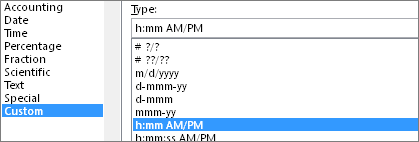
2. Set the h:mm AM/PM format.
Select both dates and press CTRL + 1 (or 
3. Subtract the two times.
In another cell, subtract the start time cell from the end time cell.
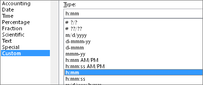
4. Set the h:mm format.
Press CTRL + 1 (or 
To calculate the time between two dates and times, you can simply subtract one from the other. However, you must apply formatting to each cell to ensure that Excel returns the result you want.
1. Type two full dates and times.
In one cell, type a full start date/time. And in another cell, type a full end date/time. Each cell should have a month, day, year, hour, minute, and a space before the AM or PM.
2. Set the 3/14/12 1:30 PM format.
Select both cells, and then press CTRL + 1 (or 
3. Subtract the two.
In another cell, subtract the start date/time from the end date/time. The result will probably look like a number and decimal. You’ll fix that in the next step.
4. Set the [h]:mm format.
Press CTRL + 1 (or 
Related Topics
DATEDIF function
NETWORKDAYS.INTL function
NETWORKDAYS
More date and time functions
Calculate the difference between two times
Watch Video – Calculate the Number of Workdays Between Two Dates
Excel has some powerful functions to calculate the number of days between two dates in Excel. These are especially useful when you’re creating Gantt charts or timelines for a proposal/project.
In this tutorial, you’ll learn how to calculate the number of days between two dates (in various scenarios):
Calculating the Total Number of Days Between Two Dates in Excel
Excel has multiple ways to calculate the days between two dates.
Using the DAYS Function
Excel DAYS function can be used to calculate the total number of days when you have the start and the end date.
You need to specify the ‘Start Date’ and the ‘End Date’ in the Days function, and it will give you the total number of days between the two specified dates.
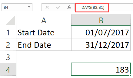
For example, suppose you have the start date is in cell B1 and End Date is in cell B2 (as shown below):
The following formula will give you the total number of days between the two dates:
=DAYS(B2,B1)
Note that you can also manually specify the dates in the Days function by putting it in double-quotes. Just make sure these dates in double-quotes is in an accepted date format in Excel.
Days function gives you the number of days between two dates. This means that if the dates are 1 Dec 2017 and 2 Dec 2017, it will return 1. If you want both the days to be counted, you need to add 1 to the result of Days function. You can read more about the Days function here.
Using the DATEDIF Function
DATEDIF function (derived from Date Difference) also allows you to quickly get the number of days between two dates. But unlike the DAYS function, it can do more than that.
You can also use the DATEDIF function to calculate the number of months or years that have elapsed in the two given dates.
Suppose you have the below dataset and you want to get the number of days between these two dates:
You can use the below DATEDIF formula to do this:
=DATEDIF(B1,B2,"D")
The above DATEDIF formula takes three arguments:
- The start date – B1 in this example
- The end date – B2 in this example
- “D” – the text string that tells the DATEDIF function what needs to be calculated.
Also note that unline the other Excel functions, when you type the DATEDIF function in Excel, it will not show the IntelliSense (the autocomplete option that helps you with the formula arguments).
If you only want to calculate the number of days between two given dates, then it’s better to use the DAYS function. DATEDIF is more suited when you want to calculate the total number of years or months that have passed in between two dates.
For example, the below formula would give you the total number of months between the two dates (in B1 and B2)
=DATEDIF(B1,B2,"M")
Similarly, the below formula will give you the total number of years between the two dates:
=DATEDIF(B1,B2,"Y")
You can read more about the DATEDIF function here. One of the common uses of this function is when you need to calculate age in Excel.
Number of Working Days Between Two Dates in Excel
Excel has two functions that will give you the total number of working days between two dates and will automatically account for weekends and specified holidays.
- Excel NETWORKDAYS function – you should use this when the weekend days are Saturday and Sunday.
- Excel NETWORKDAYS INTERNATIONAL function – use this when the weekend days are not Saturday and Sunday.
Let’s first quickly have a look at NETWORKDAYS Function syntax and arguments.
Excel NETWORKDAYS Function – Syntax & Arguments
=NETWORKDAYS(start_date, end_date, [holidays])
- start_date – a date value that represents the start date.
- end_date – a date value that represents the end date.
- [holidays] – (Optional) It is a range of dates that are excluded from the calculation. For example, these could be national/public holidays. This could be entered as a reference to a range of cells that contains the dates, an array of serial numbers that represent the dates, or a named range.
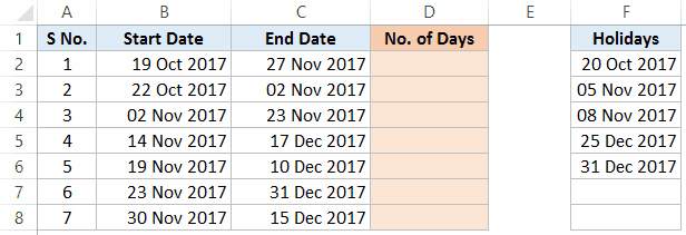
Let’s first look at an example where you want to calculate the number of working days (business days) between two dates with Saturday and Sunday as weekends.
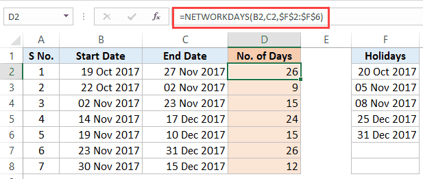
To calculate the number of working days (Column D) – when the start date, end date, and holidays are specified – use the below formula in D3 and copy for all cells:
=NETWORKDAYS(B2,C2,$F$2:$F$6)
This function works great in most cases, except the ones where the weekends are days other than Saturday and Sunday.
For example, in middle-eastern countries, the weekend is Friday and Saturday, or in some jobs, people may have a six-day workweek.
To tackle such cases, Excel has another function – NETWORKDAYS.INTL (introduced in Excel 2010).
Before I take you through the example, let’s quickly learn about the syntax and arguments of Excel NETWORKDAY INTERNATIONAL function
Excel NETWORKDAYS INTERNATIONAL Function – Syntax & Arguments
=NETWORKDAYS.INTL(start_date, end_date, [weekend], [holidays])
- start_date – a date value that represents the start date.
- end_date – a date value that represents the end date.
- [weekend] – (Optional) Here, you can specify the weekend, which could be any two days or any single day. If this is omitted, Saturday and Sunday are taken as the weekend.
- [holidays] – (Optional) It is a range of dates that are excluded from the calculations. For example, these could be national/public holidays. This could be entered as a reference to a range of cells that contains the dates or could be an array of serial numbers that represent the dates.
Now let’s see an example of calculating the number of working days between two dates where the weekend days are Friday and Saturday.
Suppose you have a dataset as shown below:
To calculate the number of working days (Column D) with the weekend as Friday and Saturday, use the following formula:
=NETWORKDAYS.INTL(B2,C2,7,$F$2:$F$6)
The third argument in this formula (the number 7) tells the formula to consider Friday and Saturday as the weekend.
Number of Weekends Between Two Dates in Excel
We can use the NETWORKDAYS function to calculate the number of weekends between two dates.
While the Networkdays function calculates the number of working days, we can also use to get the number of weekend days between two dates.
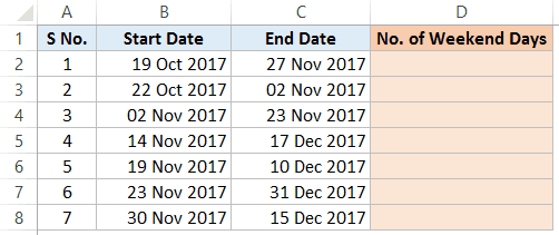
Suppose we have a dataset as shown below:
Here is the formula that will give you the total number of weekends days between the two dates:
=DAYS(C2,B2)+1-NETWORKDAYS(B2,C2)
Number of Work Days in a Part-time Job
You can use Excel NETWORKDAYS.INTL function to calculate the number of workdays in a part-time job as well.
Let’s take an example where you are involved in a project where you have to work part-time (Tuesday and Thursday only).
Here is the formula that will get this done:
=NETWORKDAYS.INTL($B$3,$C$3,"1010111",$E$3:$E$7)
Note that instead of choosing the weekend from the drop-down that’s inbuilt in the function, we have used “1010111” (in double quotes).
- 0 indicates a working day
- 1 indicates a non-working day
The first number of this series represents Monday and the last number represents Sunday.
So “0000011“ would mean that Monday to Friday are working days and Saturday and Sunday are non-working (weekend).
With the same logic, “1010111” indicates that only Tuesday and Thursday are working, and rest 5 days are non-working.
In case you have holidays (which you don’t want to get counted in the result), you can specify these holidays as the fourth argument.
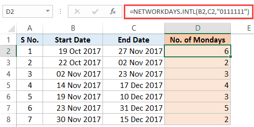
Number of Mondays Between Two Dates
To find the number of Mondays between two dates (or any other day), we can use the same logic as used above in calculating part-time jobs.
Suppose you have a dataset as shown below:
Here is the formula that will give you the number of Mondays between the two dates:
=NETWORKDAYS.INTL(B2,C2,"0111111")
In this formula, ‘0’ means a working day and ‘1’ means a non-working day.
This formula gives us the total number of working days considering that Monday is the only working day of the week.
Similarly, you can also calculate the number of any day between two given dates.
You May Also Like the Following Tutorials:
- Excel Timesheet Calculator Template.
- Convert Date to Text in Excel.
- How to Group Dates in Pivot Tables in Excel.
- How to Automatically Insert Date and Time Stamp in Excel.
- Convert Time to Decimal Number in Excel (Hours, Minutes, Seconds)
- How to SUM values between two dates in Excel
- Get Day Name from Date in Excel
- Check IF a Date is Between Two Given Dates in Excel
- How to Add Week to Date in Excel?
Summary
The Excel DAYS function returns the number of days between two dates. With a start date in A1 and end date in B1, =DAYS(B1,A1) will return the days between the two dates.
Purpose
Return value
A number representing days.
Arguments
- end_date — The end date.
- start_date — The start date.
Syntax
=DAYS(end_date, start_date)
Usage notes
The DAYS function returns the number of days between two dates. Both dates must be valid Excel dates or text values that can be coerced to dates. The DAYS function only works with whole numbers, fractional time values that might be part of a date are ignored. If start and end dates are reversed, DAYS returns a negative number. The DAYS function returns all days between two dates, to calculate working days between dates, see the NETWORKDAYS function.
Examples
With a start date in A1 and end date in A2:
=DAYS(A2,A1)
Will return the same result as:
=A2-A1
Unlike the simple formula above, the DAYS function can also handle dates in text format, as long as the date is recognized by Excel. For example:
=DAYS("7/15/2016","7/1/2016") // returns 14
The DAYS function returns the number of days between two dates. For example:
=DAYS("1-Mar-21","2-Mar-21") // returns 1
To include the end date in the count, add 1 to the result:
=DAYS("1-Mar-21","2-Mar-21")+1 // returns 2
Storing and parsing text values that represent dates should be avoided, because it can introduce errors and parsing problems. Working with native Excel dates (which are numbers) is a better approach. To create a numeric date from scratch in a formula, use the DATE function.
Notes
- The DAYS function only works with whole numbers and ignores time.
- If dates are not recognized, DAYS returns the #VALUE! error.
- If dates are out of range, DAYS returns the #NUM! error.
Author
Dave Bruns
Hi — I’m Dave Bruns, and I run Exceljet with my wife, Lisa. Our goal is to help you work faster in Excel. We create short videos, and clear examples of formulas, functions, pivot tables, conditional formatting, and charts.
Greetings, Excel pupils. Today’s class will make you Excel maestros on calculating days between two dates in Excel. Often basic tasks are trouble creators in spreadsheets and you can’t seem to find the right button, formula, or feature to smooth work out. Luckily, that bad luck charm has run out for today and we have some pretty decent formulas lined up to help us out.
Calculating days between dates is not a very foreign concept and may surface as a need for calculating lead time, timelines, deadlines, etc. In this tutorial, we have 3 easy formulas (simple subtraction and the DAYS and DATEFIF functions) for calculating the days between two dates. You will also be briefed on how to use the NETWORKDAYS function to compute weekend days and weekdays and how to include certain holidays in the computations.
Our guide includes practical application of these formulas using a dummy case example. Lead with example they say and lead with example we shall.
Example
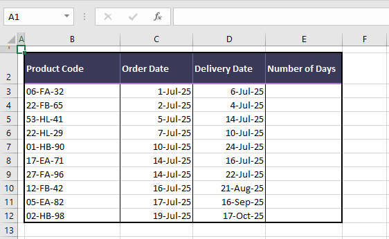
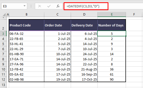
Here is the example using which we will test all our formulas. We have 10 products with their order dates in column C and delivery dates in column D.
The aim is to calculate the number of days between the customer placing the order and the product being delivered.
Pro Tip: For working dynamically with the current date, you can use the TODAY function in place of the date in any formula. The argument to use the TODAY function in place of a date is:
=TODAY()
The ease of using the TODAY function is that it will be a dynamic argument, updating with the current date and recalculating the formula accordingly.
Now ready to see what’s in store today?
Let’s get calculating!
Subtracting the Dates
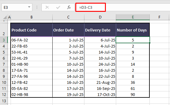
Here begin our experiments to calculate days between two dates in Excel. We’ll give the first go to the simplest of all the formulas as it uses no functions; just elementary math. Narrowing that down even further, we will subtract the dates to find the days between them. This is how we’re doing it:
=D3-C3
As a rule of thumb of subtraction, the smaller number is deducted from the larger number. This also goes for our dates; the order date in cell C3 is subtracted from the delivery date in D3 which is the later date. This gives us an outcome of ‘5’ i.e. 5 days.
Since the first pair of dates have behaved, let’s apply the formula to the rest of the dates to calculate the days between the two dates:
Using DAYS Function
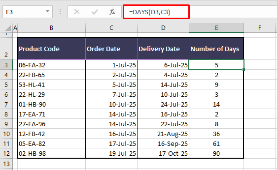
The next method of calculating days between two dates uses the DAYS function. The DAYS function takes the end date and start date to return the number of days between the two dates. That suits us! Let’s apply the following DAYS function formula to our example:
=DAYS(D3,C3)
D3 makes the end date and C3 makes the start date for the DAYS function. DAYS calculates the days between the two dates and returns 5 as the result. No fuss, no frills, we have the results of the DAYS function in our case example:
Using DATEDIF Function
Now we’ll see what the DATEDIF function can do for us while we’re trying to calculate the days between two dates. This elusive function can compute the number of days, months, or years between two dates. Along with the two dates, the DATEDIF function takes one more argument i.e. the unit which defines what the function should return (e.g. “D” for returning the number of days, “M” for returning the number of complete months).
Since it seems to get the job done, what’s so elusive about this function? Being an undocumented function, the DATEDIF function makes no effort to appear in the Excel Formula AutoComplete. If this piques your curiosity, the syntax and the ins and outs of the DATEDIF function can be found here.
Got the idea? Now we can show you how to apply DATEDIF to our case example and calculate the days between two dates:
=DATEDIF(C3,D3,"D")
Following the syntax, we’ve given the DATEFIF function a start date (C3), an end date (D3), and a unit (D) so that DATEDIF calculates the number of days between the two given dates. The formula has been extended to the list of dates and we have the output below:
Calculating the Number of Working Days Between Two Dates
When trying to get the number of days between two dates, you may be calculating from a work point of view. Hence, it will be important to take the weekends into account (or out of account, actually) and deduct them to arrive at the number of working days between two dates.
Thankfully, that’s not something you need to do yourself; we have the NETWORKDAYS functions for that. Now it depends what day(s) the weekend falls for you. That’s still not a problem. The NETWORKDAYS function by default considers Saturday and Sunday as the weekend days. For any other weekend days, we will show you how to use the NETWORKDAYS.INTL function.
Calculating the Number of Working Days (Weekend is Saturday and Sunday)
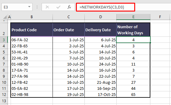
The NETWORKDAYS function returns the number of whole workdays between two dates. Let’s give this formula a run and see how things turn out:
=NETWORKDAYS(C3,D3)
The two dates given to NETWORKDAYS are C3 and D3. Now, we can end the formula here and we’d have the number of working days computed like below:
But let’s throw another spanner into the works which is an optional feature of NETWORKDAYS itself. The new formula only adds the third argument and will be:
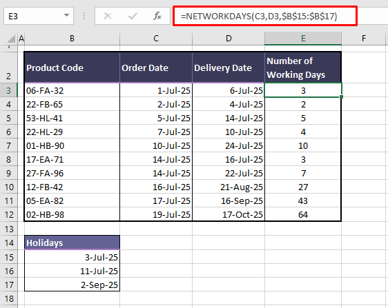
=NETWORKDAYS(C3,D3,$B$15:$B$17)
If NETWORKDAYS is supplied with a range of dates as a reference, the function can also exclude them from the count. Therefore, we have a small list of holidays in B15:B17 and we have referred this range in the formula as a third argument. The range is locked into an absolute reference in the formula with $ signs (to apply, position the blinking cursor before, after, or in the middle of the cell reference and press the F4 key).
Now the results will change slightly, the NETWORKDAYS function having to exclude holidays from the calculation of days between the dates:
Notice the change? The number of working days in the instances where the holidays are falling, is a day less than before the holidays were included.
Calculating the Number of Working Days (Weekend is not Saturday and Sunday)
Your weekend may not fall on Saturday and Sunday or you may have a single-day weekend depending on your job or location. Excel has understanding of these (and sympathizes with the latter) and therefore has the NETWORKDAYS.INTL function for accommodating weekends falling on different days.
The NETWORKDAYS.INTL function requires one more argument than the NETWORKDAYS function and that is the weekend parameter. NETWORKDAYS.INTL will return the number of full workdays between two dates according to the selected weekend parameter. Let’s have the formula:
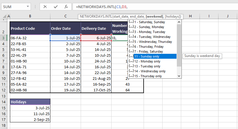
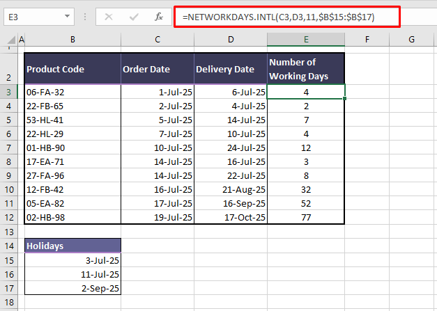
=NETWORKDAYS.INTL(C3,D3,11,$B$15:$B$17)
The formula is a copy of the one used for NETWORKDAYS except for the added argument for the weekend days. The NETWORKDAYS.INTL function will calculate the days between C3 and D3, taking into account e.g. Sunday as the weekend days and the given holidays in B15:B17. When typing the formula, the Formula AutoComplete will display the parameters for the selection of the weekend days:
The formula returns these results with our case example:
Recommended Reading: How to calculate business days between two dates
Calculating the Number of Weekends (Weekend is Saturday and Sunday)
We just saw how to calculate the number of weekdays and now we will calculate the number of weekend days between two dates. This will require the NETWORKDAYS function with the DAYS function.
The concept is to calculate the total number of days between two dates using the DAYS function and deduct the number of working days from it, computed using the NETWORKDAYS function. By now we know how both functions work so let’s move onto the formula:
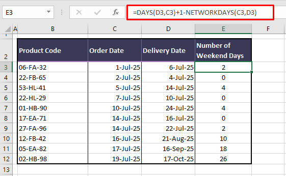
=DAYS(D3,C3)+1-NETWORKDAYS(C3,D3)
The DAYS function starts off by calculating the number of days between the dates in C3 and D3. This part of the formula returns 5 as the total days. We are adding 1 day here as the DAYS function calculates the difference between the two dates without including a full day. 5+1 brings us to 6 days.
In the next part of the formula, we calculate the working days between C3 and D3 using the NETWORKDAYS function. This gives us 4 working days. The result of NETWORKDAYS is deducted from that of DAYS i.e. 6-4 and we arrive at the weekend days as 2 days.
Our case example with this formula looks like:
Calculating the Number of Weekends (Weekend is not Saturday and Sunday)
And again, if your weekend falls on a different day, the NETWORKDAYS.INTL function can be used interchangeably in this formula. The new formula would be:
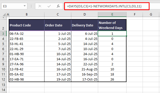
=DAYS(D3,C3)+1-NETWORKDAYS.INTL(C3,D3,11)
The NETWORKDAYS function has been swapped for the NETWORKDAYS.INTL function and the weekend parameter has been added, making Sundays the only weekend day. This is how the results change using the above formula:
Class dismissed! That’s what we had on easy ways to calculate days between two dates in Excel. We also covered excluding holidays from the count and how to calculate working days and weekend days between the dates. We’d like to see you back for the next lesson. Topic hint: Excel matter!
Calculating the number of days between two dates in Excel is a popular operation performed in different scenarios.
For example, project managers use it to measure performance against milestones and accountants use it to track aging receivables.
This tutorial shows you how to calculate the number of days between two dates in Excel in different situations.
How to Calculate the Overall Number of Days Between Two Dates
In this first scenario, I will show you how to calculate the total number of days between two given dates. These would include all days, i.e., working days, weekends, and holidays.
Method #1: Use the Subtraction Method
Excel stores dates as sequential serial numbers.
This allows us to subtract the start date from the end date to get the total number of days between the two dates.
Below I have a data set where I have the start date and the end date, and I’ll create the total number of days between these two dates

We use the following steps:
- Select cell D2 and type in the following formula:
=C2-B2

- Press Enter on the keyboard or click the Enter button on the Formula Bar.

- Double-click the fill handle or drag down the fill handle to copy the formula down the column.

Also read: How to Get Total Days in Month in Excel?
Method #2: Use the DATEDIF Function
The DATEDIF function is a legacy function maintained in Excel for the purpose of compatibility with Lotus 1-2-3.
The function calculates the number of years, days, or months between two dates. When you start to type it in a cell it does not appear as part of IntelliSense and must be entered manually.
Using the dataset in the previous illustration, we proceed as follows:
- Select cell D2 and type in the following formula:
=DATEDIF(B2,C2,"d")

- Press Enter key on the keyboard or click the Enter button on the Formula Bar.
- Double-click or drag down the fill handle to copy the formula down the column.

Let me quickly explain how this works.
Below is the syntax of the DATEDIF function
DATEDIF(start_date,end_date,unit)
The DATEDIF function has the following arguments:
- The start_date is a required argument and stands for the starting date of a given period. In our example, it represents the start date of the project.
- The end_date is a required argument and stands for the last date of a given period. In our example, it stands for the last date of the project.
- The unit argument is a required argument, and it stands for the type of data you want the function to return. In our example, we want the function to return the number of days and therefore we use the “d” unit.
Note: You can also use the DATEDIF function to calculate the total number of months or number of years between two given dates. to do this, instead of using “d”, you can use “m” or “y”
Also read: Calculate Days Left in the Year (Formula)
Method #3: Use the DAYS Function
The DAYS function returns the overall number of days between two date values.
Using the dataset in the previous illustration, we proceed as follows:
- Select cell D2 and type in the following formula:
=DAYS(C2,B2)

- Press Enter key on the keyboard or click the Enter button on the Formula Bar.
- Double-click the fill handle or drag down the fill handle to copy the formula down the column.

Below is the syntax of the DAYS function
DAYS(end_date,end_date)
The DAYS function has the following arguments:
- The start_date. It is a required argument and stands for the starting date of a given period. In our illustration, it represents the start date of the project.
- The end_date. It is a required argument and stands for the last date of a given period. In our illustration, it stands for the last date of the project.
How to Compute the Overall Number of Workdays Between Two Dates
Operations are normally shut down during weekends. You would want to exclude weekends when figuring out the number of workdays between two dates.
Below is the data set that I’m going to use for the illustration. It has the start date and the end date, and I want to calculate the total number of working days between these two dates (excluding the weekend dates).

Method #1: Use the NETWORKDAYS Function to Exclude Saturdays and Sundays
The NETWORKDAYS function returns the number of days between two dates excluding Saturdays and Sundays. It can also optionally exclude specified holidays but we shall illustrate that in the next method.
Below are steps to get the total number of days between two dates while excluding Saturday and Sunday:
- Select cell D2 and type in the following formula:
=NETWORKDAYS(B2,C2)

- Press Enter key on the keyboard or click the Enter button on the Formula Bar.
- Double-click the fill handle or drag down the fill handle to copy the formula down the column.

Below is the syntax of the NETWORKDAYS function:
NETWORKDAYS(start_date,end_date,[holidays])
The NETWORDAYS function has the following arguments:
- The start_date. It is a required argument and stands for the starting date of a given period. In our illustration, it represents the start date of the project.
- The end_date. This argument is a required argument and stands for the last date of a given period. In our illustration, it stands for the last date of the project.
- The [holidays]. This argument is an optional argument. It represents a range of one or more dates such as federal and state holidays that are excluded from the working calendar. The dates to be excluded can be entered as a named range, a range of cells containing the dates, or a list of serial numbers representing the dates.
Method #2: Use the NETWORKDAYS Function to Exclude Saturdays, Sundays, and Holidays
The NETWORDAYS function by default excludes Saturdays and Sundays in its calculation.
If you want it to also exclude holidays, you have to pass to the function the dates to exclude.
The dates to be excluded can be entered as a named range, a range of cells containing the dates, or a list of serial numbers representing the dates.
Below I have a data set where I have the start date and the end date, and I also have a list of holidays. I want to calculate the total number of days between the start and the end date while excluding the holidays and weekend days.

Below are the steps to do this:
- Select cell D2 and type in the formula below:
=NETWORKDAYS(B2,C2,$F$2:$F$5)
Note: Press F4 after typing in range F2:F5 to lock it down and make it an absolute reference.

- Press Enter key on the keyboard or click the Enter button on the Formula Bar.
- Double-click the fill handle or drag down the fill handle to copy the formula down the column.

While the NETWORKDAYS function is already built to take the start date and the end date and give you the total number of days between these two dates while excluding Saturdays and Sundays.
In this above example, we have also used the third optional argument that refers to the dates that are holidays.
So the final result that we get would give us the total number of days between the start date and the end date while excluding the weekend days and the holidays.
In case a holiday occurs on a weekend day, the function is smart enough to only recognize this and not exclude it twice.
Method #3: Use the NETWORKDAYS.INTL Function to Exclude Custom Weekends
One limitation of using the NETWORKDAYS function is that it defaults to excluding Saturday and Sunday.
In some countries or regions, weekends are Fridays and Saturdays or another combination of days.
In other situations, the weekend may be only Sunday or some other day. The NETWORKDAYS.INTL function takes care of such scenarios.
The NETWORKDAYS.INTL function returns the number of days between two dates excluding custom weekends. It can also optionally exclude holidays.
The syntax of the NETWORKDAYS.INTL function:
NETWORKDAYS.INTL(start_date,end_date,[weekend],[holidays])
The function has the following arguments:
- start_date. It is a required argument. It represents a date value that is the starting date of a given period.
- end_date. It is a required argument. It represents a date value that is the ending date of a given period.
- [weekend]. It is an optional argument. It specifies the days of the week that are weekend days. The days can be specified by a weekend number or a string that shows when weekends occur. If this argument is omitted, the weekend days of Saturday and Sunday are assumed.
The weekend numbers range from 1 to 17. Each number represents a weekend day or weekend day.


- [holidays]. It is an optional argument. It represents a range of one or more dates such as federal and state holidays that are excluded from the working calendar. The dates to be excluded can be entered as a named range, a range of cells containing the dates, or a list of serial numbers representing the dates.
We give an example of calculating the number of working days between two dates excluding Friday and Saturday as weekend days.
We use the following dataset:

We use the steps below:
- Select cell D2 and type in the formula below:
=NETWORKDAYS.INTL(B2,C2,7)
Note: The third argument is weekend number 7 which represents the weekend days of Friday and Saturday.

- Press Enter key on the keyboard or click the Enter button on the Formula Bar.
- Double-click the fill handle or drag down the fill handle to copy the formula down the column.

The above formula gives us the total number of days between the start and the end date, while excluding all the Fridays and Saturdays.
Method #4: Use the NETWORKDAYS.INTL to Exclude Custom Weekends and Holidays
The NETWORKDAYS.INTL function returns the number of days between two dates excluding custom weekends. It can also optionally exclude holidays.
We give an example of calculating the number of working days between two dates excluding the weekend days of Wednesday and Thursday and holidays in a given range.
We use the following dataset:

We use the following steps:
- Select cell D2 and type in the following formula:
=NETWORKDAYS.INTL(B2,C2,5,$F$2:$F$5)

- Press Enter key on the keyboard or click the Enter button on the Formula Bar.
- Double-click the fill handle or drag down the fill handle to copy the formula down the column.

The above formula gives us the total number of days between the start and the end date, while excluding the days that occur on Wednesdays and Thursdays and holidays
How to Calculate the Number of Custom Workdays Between Two Dates
We can use the NETWORKDAYS.INTL function to calculate the number of custom workdays between two dates.
Custom workdays could be the number of days one works at a part-time job.
Method #1: Use the NETWORKDAYS.INTL Function to Calculate the Number of Part-time Workdays
We give an example of calculating the number of custom workdays between two dates where an employee works part-time at a job on Mondays and Fridays only.
The dataset below is used in our example:

- Select cell D2 and type in the following formula:
=NETWORKDAYS.INTL(B2,C2,"0111011")
Note: Instead of entering a weekend number in the third argument, we enter a string of seven characters. Each character stands for a day of the week beginning with Monday. Character 1 stands for a non-workday and 0 represents a workday. Therefore “0111011” represents the workdays of Monday and Friday.

- Press Enter key on the keyboard or click the Enter button on the Formula Bar.
- Double-click the fill handle or drag down the fill handle to copy the formula down the column.

Note: If we have holidays we want to be excluded from the number of part-time workdays, we can pass the days to the function as the fourth argument.
Method #2: Use NETWORKDAYS.INTL Function to Calculate the Number of Fridays (or any other day) Between Two Dates
We can use the NETWORKDAYS.INTL function to calculate the number of specified days of the week between two dates.
Suppose we want to find out the number of Fridays between two dates. We use the following dataset to explain how this can be achieved.

We use the steps below:
- Select cell D2 and type in the following formula:
=NETWORKDAYS.INTL(B2,C2,"1111011")
Note: Instead of entering a weekend number in the third argument, we enter a string of seven characters. Each character stands for a day of the week beginning with Monday. Character 1 stands for a non-workday and 0 represents a workday. Therefore “1111011” represents the workday of Friday.

- Press Enter key on the keyboard or click the Enter button on the Formula Bar.
- Double-click the fill handle or drag down the fill handle to copy the formula down the column.

Note: The logic behind the argument of the seven-character string can be applied to calculate the total number of any other day between two dates.
How to Compute the Overall Number of Weekend Days Between Two Dates
Sometimes we may want to find out the number of weekend days between two dates.
We can use the combination of the DAYS function and the NETWORKDAYS function to calculate the number of weekend days between two dates.
The syntax of these two functions and their arguments have been explained previously in this tutorial.
The dataset below is used in our illustration:

We proceed as follows:
- Select cell D2 and type in the following formula:
=DAYS(C2,B2)+1-NETWORKDAYS(B2,C2)
Note: We add 1 to the days returned by the DAYS function so as to include both the start date and the end date.
The logic of the formula is that the total number of workdays between two dates is subtracted from the total number of days between the two dates (the start date and end date inclusive).
The result is the number of weekend days between the two dates.

- Press Enter key on the keyboard or click the Enter button on the Formula Bar.
- Double-click the fill handle or drag down the fill handle to copy the formula down the column.

In this tutorial, I showed you different scenarios where you can use different formulas to calculate the number of days between two given dates.
I covered how you can calculate the total number of days between us start and the end date, or you can calculate only the working days using functions such as NETWORKDAYS and NETWORKDAYS.INTL.
I also covered how to calculate the number of working days when you’re in a part-time job, or you want to only calculate the number of specific days between the two dates (such as the number of Fridays or the number of Mondays between two given dates).
Other articles you may also like:
- How to Calculate the Number of Months Between Two Dates in Excel?
- How to Change Date and Time to Date in Excel (4 Easy Ways)
- Find Last Monday of the Month Date in Excel (Easy Formula)
- Using IF Function with Dates in Excel (Easy Examples)
- How to Convert Days to Years in Excel (Simple Formulas)
- How to Convert Date to Day of Week in Excel (3 Easy Ways)
- How to Add Days to a Date in Excel









![Format Cells dialog, Custom command, [h]:mm type](https://support.content.office.net/en-us/media/2edbd461-d4c5-49a7-a5a2-b6d9329c0411.png)

