
Excel for Microsoft 365 Excel for Microsoft 365 for Mac Excel for the web Excel 2021 Excel 2021 for Mac Excel 2019 Excel 2019 for Mac Excel 2016 Excel 2016 for Mac Excel 2013 Excel 2010 Excel 2007 Excel for Mac 2011 Excel Starter 2010 More…Less
Use Excel’s DATE function when you need to take three separate values and combine them to form a date.
The DATE function returns the sequential serial number that represents a particular date.
Syntax: DATE(year,month,day)
The DATE function syntax has the following arguments:
-
Year Required. The value of the year argument can include one to four digits. Excel interprets the year argument according to the date system your computer is using. By default, Microsoft Excel for Windows uses the 1900 date system, which means the first date is January 1, 1900.
Tip: Use four digits for the year argument to prevent unwanted results. For example, «07» could mean «1907» or «2007.» Four digit years prevent confusion.
-
If year is between 0 (zero) and 1899 (inclusive), Excel adds that value to 1900 to calculate the year. For example, DATE(108,1,2) returns January 2, 2008 (1900+108).
-
If year is between 1900 and 9999 (inclusive), Excel uses that value as the year. For example, DATE(2008,1,2) returns January 2, 2008.
-
If year is less than 0 or is 10000 or greater, Excel returns the #NUM! error value.
-
-
Month Required. A positive or negative integer representing the month of the year from 1 to 12 (January to December).
-
If month is greater than 12, month adds that number of months to the first month in the year specified. For example, DATE(2008,14,2) returns the serial number representing February 2, 2009.
-
If month is less than 1, month subtracts the magnitude of that number of months, plus 1, from the first month in the year specified. For example, DATE(2008,-3,2) returns the serial number representing September 2, 2007.
-
-
Day Required. A positive or negative integer representing the day of the month from 1 to 31.
-
If day is greater than the number of days in the month specified, day adds that number of days to the first day in the month. For example, DATE(2008,1,35) returns the serial number representing February 4, 2008.
-
If day is less than 1, day subtracts the magnitude that number of days, plus one, from the first day of the month specified. For example, DATE(2008,1,-15) returns the serial number representing December 16, 2007.
-
Note: Excel stores dates as sequential serial numbers so that they can be used in calculations. January 1, 1900 is serial number 1, and January 1, 2008 is serial number 39448 because it is 39,447 days after January 1, 1900. You will need to change the number format (Format Cells) in order to display a proper date.
Syntax: DATE(year,month,day)
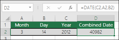
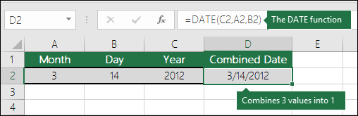
For example: =DATE(C2,A2,B2) combines the year from cell C2, the month from cell A2, and the day from cell B2 and puts them into one cell as a date. The example below shows the final result in cell D2.
Need to insert dates without a formula? No problem. You can insert the current date and time in a cell, or you can insert a date that gets updated. You can also fill data automatically in worksheet cells.
-
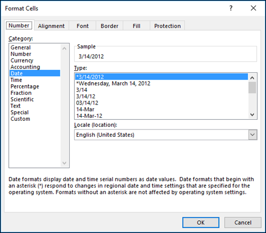
Right-click the cell(s) you want to change. On a Mac, Ctrl-click the cells.
-
On the Home tab click Format > Format Cells or press Ctrl+1 (Command+1 on a Mac).
-
3. Choose the Locale (location) and Date format you want.
-
For more information on formatting dates, see Format a date the way you want.

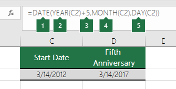
You can use the DATE function to create a date that is based on another cell’s date. For example, you can use the YEAR, MONTH, and DAY functions to create an anniversary date that’s based on another cell. Let’s say an employee’s first day at work is 10/1/2016; the DATE function can be used to establish his fifth year anniversary date:
-
The DATE function creates a date.
=DATE(YEAR(C2)+5,MONTH(C2),DAY(C2))
-
The YEAR function looks at cell C2 and extracts «2012».
-
Then, «+5» adds 5 years, and establishes «2017» as the anniversary year in cell D2.
-
The MONTH function extracts the «3» from C2. This establishes «3» as the month in cell D2.
-
The DAY function extracts «14» from C2. This establishes «14» as the day in cell D2.
If you open a file that came from another program, Excel will try to recognize dates within the data. But sometimes the dates aren’t recognizable. This is may be because the numbers don’t resemble a typical date, or because the data is formatted as text. If this is the case, you can use the DATE function to convert the information into dates. For example, in the following illustration, cell C2 contains a date that is in the format: YYYYMMDD. It is also formatted as text. To convert it into a date, the DATE function was used in conjunction with the LEFT, MID, and RIGHT functions.

-
The DATE function creates a date.
=DATE(LEFT(C2,4),MID(C2,5,2),RIGHT(C2,2))
-
The LEFT function looks at cell C2 and takes the first 4 characters from the left. This establishes “2014” as the year of the converted date in cell D2.
-
The MID function looks at cell C2. It starts at the 5th character, and then takes 2 characters to the right. This establishes “03” as the month of the converted date in cell D2. Because the formatting of D2 set to Date, the “0” isn’t included in the final result.
-
The RIGHT function looks at cell C2 and takes the first 2 characters starting from the very right and moving left. This establishes “14” as the day of the date in D2.
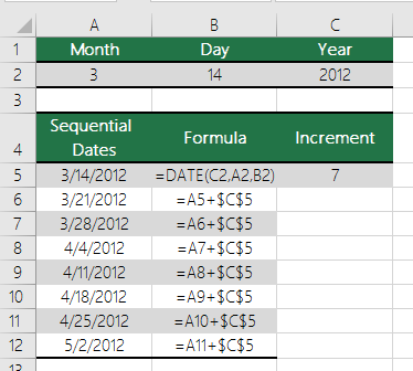
To increase or decrease a date by a certain number of days, simply add or subtract the number of days to the value or cell reference containing the date.
In the example below, cell A5 contains the date that we want to increase and decrease by 7 days (the value in C5).
See Also
Add or subtract dates
Insert the current date and time in a cell
Fill data automatically in worksheet cells
YEAR function
MONTH function
DAY function
TODAY function
DATEVALUE function
Date and time functions (reference)
All Excel functions (by category)
All Excel functions (alphabetical)
Need more help?
Want more options?
Explore subscription benefits, browse training courses, learn how to secure your device, and more.
Communities help you ask and answer questions, give feedback, and hear from experts with rich knowledge.
Excel spreadsheets provide the ability to work with various types of textual and numerical information. Date processing is also available. In this case, there may be a need to extract from the general meaning of a specific number, for example, a year. There are separate functions for this: YEAR, MONTH, DAY and DAY.
Examples of using functions for date processing in Excel
Excel tables store dates that are presented as a sequence of numeric values. It begins on January 1, 1900. This date will correspond to the number 1. At the same time, January 1, 2009 is laid down in the tables, as the number 39813. This is the number of days between the two designated dates.
The function YEAR is used similarly to the adjacent:
- MONTH;
- DAY;
- WEEKDAY.
All of them display numerical values corresponding to the Gregorian calendar. Even if in the Excel spreadsheet, the Hijra calendar was chosen to display the entered date, then when isolating the year and other composite values by functions, the application will present a number that is equivalent to the Gregorian system of chronology.
To use the YEAR function, you need to enter into the cell the following function formula with one argument:
=YEAR(cell address with date in numeric format)
The function argument is required. It can be replaced by «date_number_number». In the examples below, you can clearly see this. It is important to remember that when displaying the date as text (automatic orientation on the left edge of the cell), the YEAR function will not be executed. Its result will be the # SIGN. Therefore, formatted dates must be presented in a numerical version. Days, months and year can be separated by a dot, slash or comma.
Consider an example of working with the YEAR function in Excel. If we need to get a year from the original date, the function AVAILABLE will not help us since it does not work with dates, but only with text and numeric values. To separate the year, month or day from the full date for this, Excel provides functions for working with dates.
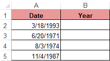
Example: There is a table with a list of dates and in each of them it is necessary to separate the value of only the year.
We introduce the original data in Excel.
To solve the problem, it is necessary to enter the formula in the cells of column B:
=YEAR(the address of the cell, from the date of which you need to isolate the year value)
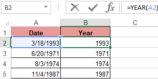
As a result, we extract years from each date.
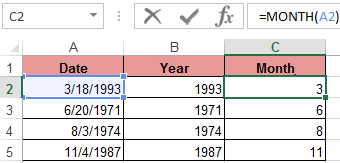
A similar example of the MONTH function in Excel:
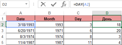
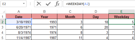
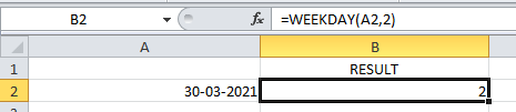
An example of working with functions DAY and WEEKDAY. The DAY function gets to calculate from the date the number of any day:
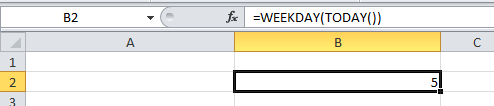
WEEKDAY function returns the number of the day of the week (1-Monday, 2-Tuesday …, etc.) for any date:
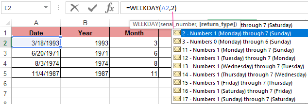
In the second optional argument of the WEEKDAY function, the number 2 may specified for our day of the week countdown format (Monday-1 through Sunday-7):
If you omit the second optional argument, then the default format will be used (English from Sunday-1 to Saturday-7).
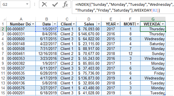
Create a formula of the combination of the functions INDEX and WEEKDAY:
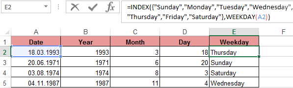
We obtain a more understandable form of the implementation of this function.
Examples of the practical use of functions for working with dates
These primitive functions are very useful when grouping data by: years, months, days of the week, and specific days.
Suppose we have a simple sales report:
We need to quickly organize data for visual analysis without using pivot tables. To do this, we will bring the report into a table where it is convenient and quickly to group data by year, month and day of the week:
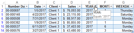
Now we have a tool to work with this sales report. We can filter and segment data by specific time criteria:
In addition, you can make a histogram to analyze the best-selling days of the week, to understand which day of the week has the largest number of sales:
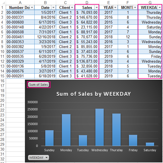
In this form, it is very convenient to segment sales reports for long, medium and short periods of time.
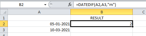
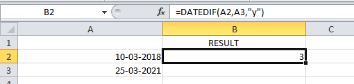
It should be immediately noted that in order to get the difference between the two dates, none of the above functions will help us. For this task, you should use a specially designed function DATEDIF:
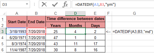
Download examples fo functions YEAR MONTH DAY WEEKDAY and DATEDIF
The type of values in the date cells requires a special approach to data processing. Therefore, you should use the appropriate type of function in Excel.
The DATE function creates a date using individual year, month, and day arguments. Each argument is provided as a number, and the result is a serial number that represents a valid Excel date. Apply a date number format to display the output from the DATE function as a date.
In general, the DATE function is the safest way to create a date in an Excel formula, because year, month, and day values are numeric and unambiguous, in contrast to text representations of dates which can be misinterpreted.
Note: to move an existing date forward or backward in time, see the EDATE and EOMONTH.
Example #1 — hard-coded numbers
For example, you can use the DATE function to create the dates January 1, 1999, and June 1, 2010 with the following syntax:
=DATE(1999,1,1) // returns Jan 1, 1999
=DATE(2010,6,1) // returns Jun 1, 2010
Example #2 — cell reference
The DATE function is useful for assembling dates that need to change dynamically based on other inputs in a worksheet. For example, with 2018 in cell A1, the formula below returns the date April 15, 2018:
=DATE(A1,4,15) // Apr 15, 2018
If A1 is then changed to 2019, the DATE function will return a date for April 15, 2019.
Example #3 — with SUMIFS, COUNTIFS
The DATE function can be used to supply dates as inputs to other functions like SUMIFS or COUNTIFS, since you can easily assemble a date using year, month, and day values that come from a cell reference or formula result. For example, to count dates greater than January 1, 2019 in a worksheet where A1, B1, and C1 contain year, month, and day values (respectively), you can use a formula like this:
=COUNTIF(range,">"&DATE(A1,B1,C1))
The result of COUNTIF will update dynamically when A1, B1, or C1 are changed.
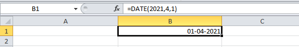
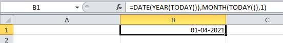
Example #4 — first day of current year
To return the first day of the current year, you can use the DATE function like this:
=DATE(YEAR(TODAY()),1,1) // first of year
This is an example of nesting. The TODAY function returns the current date to the YEAR function. The YEAR function extracts the year and returns the result to the DATE function as the year argument. The month and day arguments are hard-coded as 1. The result is the first day of the current year, a date like «January 1, 2021».
Note: the DATE function actually returns a serial number and not a formatted date. In Excel’s date system, dates are serial numbers. January 1, 1900 is number 1 and later dates are larger numbers. To display date values in a human-readable date format, apply the number format of your choice.
Notes
- The DATE function returns a serial number that corresponds to an Excel date.
- Excel dates begin in the year 1900. If year is between zero and 1900, Excel will add 1900.
- The DATE function accepts numeric input only and will return #VALUE if given text.
There are many functions in Microsoft Excel that may be used to work with dates and timings in Excel. Each function completes a straightforward task, but by combining numerous functions into a single formula, you may handle trickier and more complicated problems. The purpose of discussing DATE functions in Excel is to help different people to perform more complex and challenging tasks by combining several functions within one formula.
The DATE function is used to calculate dates in Excel. Excel provides different functions to work with dates & times such as TODAY, NOW, WEEKDAY, EOMONTH, etc. which we will discuss here with examples.
1. DATE Function in Excel
It will return the date in serial number based on the year, month, or day value as provided.
Syntax:
DATE(year,month,day)
Arguments:
- Year – This argument includes – 1 to 4-digit values. Excel understands this ‘year’ argument according to the date system of the local computer which we use. For example- Excel windows uses the 1900 date system by default which means DATE (21,2,6) gives the result as 06-02-1921.
- Month – This argument includes a positive or negative integer that represents the month of the year from January to December.
- Day – This argument also includes a positive or negative integer representing the day of the month from 1 to 31.
Excel Date Function Example 1:
Excel Date Function Example 2:
It will return on the first day of the current year & month.
Excel Date Function Example 3:
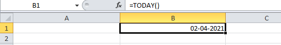
2. TODAY Function in Excel
The TODAY() function name suggests it will return today’s date, and it has no arguments.
Syntax:
TODAY()
Example1:
Here we will print the current date and also add 10 days to the current date.
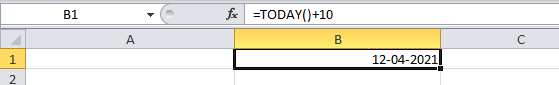
Example 2:
To add 10 days to Today’s date.
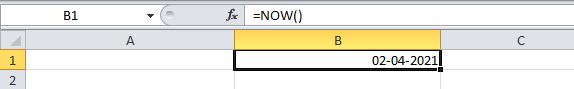
3. NOW Function in Excel
This function returns the current date as well as the time & doesn’t have any arguments.
Syntax:
NOW()
Example:
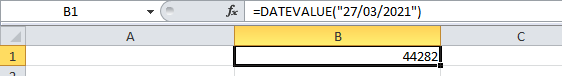
4. DATEVALUE Function
It converts the date in text format to a serial number, which can be represented as a date.
Syntax:
DATEVALUE(date_text)
Arguments:
1. date_text – This argument is a text that represents the date in Excel date format.
Example:
5. TEXT Function
It converts any numeric value not only dates to a text string. Through this function, we can change the date to text strings in a variety of formats.
Syntax:
TEXT(value,format_text)
Arguments:
1. value: The value that is to be converted.
2. format_text: The format in which you want to output the date value.
These are the different formats used in the TEXT function to change dates to text strings.
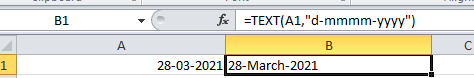
Example 1:
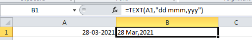
Example 2:
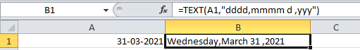
Example 3:
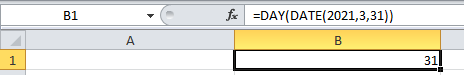
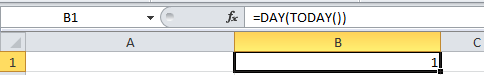
6. DAY Function
It returns the day of a month, i.e. integer from 1 to 31.
Syntax:
DAY(serial_number)
Arguments:
1. serial_number: This value represents the day of the month you want to find. E.g: 5th day of June
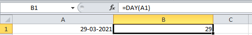
Example 1:
Example 2:
The DAY(TODAY()) function returns the day of today’s date, as shown below:
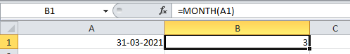
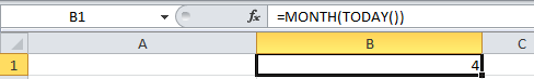
7. MONTH Function
This function returns the month of the given date as an integer from 1 to 12 (January to December).
Syntax:
MONTH(serial_number)
Arguments:
1. serial_number: This value represents the date for which you want to find the month.
Example:
The MONTH(TODAY()) function returns the month of today’s date.
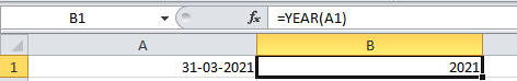
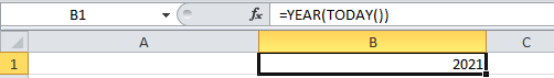
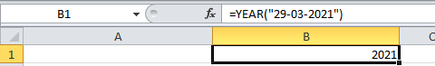
8. YEAR Function
It returns the year of a specified date.
Syntax:
YEAR(serial_number)
Arguments:
1. serial_number: The date to be specified.
Example 1:
Example 2:
Example 3:
9. EOMONTH Function
This function returns the last day of the month after adding a specified number of months to a given date.
Syntax:
EOMONTH(start_date,months)
Arguments:
1. start_date: In this argument, the date should be written in date format, not in the text.
2. months: In this argument, if a positive integer is given then corresponding months can be added to the start date & if a negative integer is given then the corresponding months can be subtracted from the start date.
Example 1:
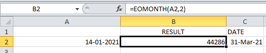
Example 2:
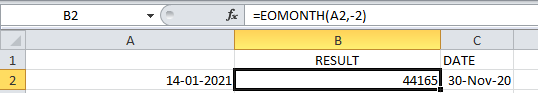
Example 3:
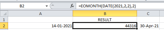
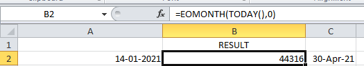
The EOMONTH(TODAY(),0) function returns the last day of the current month.
10. WEEKDAY Function
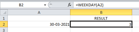
This function returns the day of the week as a number from 1 to 7 (Sunday to Saturday) according to the specified date.
Syntax:
WEEKDAY(serial_number,return_type)
Arguments:
1. serial_number: It can be a date or the cell that contains the date.
2. return_type: It is optional, as it specifies which day should be considered as the first day of the week.
NOTE: 1st day of the week is by default Sunday.
Example 1:
Example 2:
In the below example, 2 is given as return_type i.e. Monday is referred to as the first day of the week.
Example 3:
Here the day of today’s (01-04-2021) date is the result & the default value (Sunday) is considered here because no return_type is given.
11. DATEDIF Function
This function calculates the difference between two dates in days, months, or years. For calculating the difference b/w dates which time interval should be used depends on the letter which we specify in our last argument i.e. at the unit.
Syntax:
DATEDIF(start_date,end_date,unit)
Arguments:
1. start_date: The start date for evaluating the difference.
2. end_date: The end Date for evaluating the difference.
Example 1:
Example 2:
Example 3:
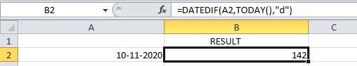
Here “m”,”y”,”d” means month, year & date. In the first example, the difference between dates is calculated by months, second by year & third by date.
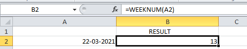
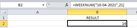
12. WEEKNUM Function
It returns the week number based on the specified date, i.e. from 1 to 52 weeks of the year.
Syntax:
WEEKNUM(serial_number,firstday_ofweek)
Arguments:
1. serial_number: This is the date for which we want the week number.
2. firstday_ofweek: This is an optional argument that specifies which numbering system should be considered & which day of the week can be treated as the start of the week, Default(omitted) is 1. The table below is the parameters that can be given in firstday_ofweek argument.
First Day of the Week Start Table:
| 1 | Sunday | 1 |
| 2 | Monday | 1 |
| 11 | Monday | 1 |
| 12 | Tuesday | 1 |
| 13 | Wednesday | 1 |
| 14 | Thursday | 1 |
| 15 | Friday | 1 |
| 16 | Saturday | 1 |
| 17 | Sunday | 1 |
| 21 | Monday | 2 |
Example 1:
Example 2:
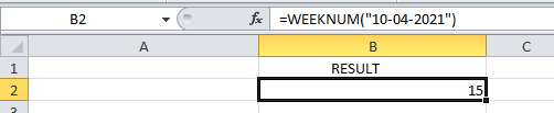
Example 3:
In the below example,21 is given as the second argument which means Monday is taken as the first day of the week & in the above example, the result shown is 15 but taking 21 as the first_dayofweek means Monday is the first day, the result is 14.
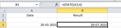
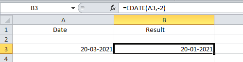
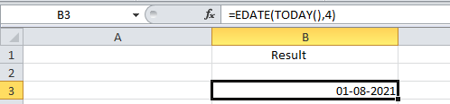
13. EDATE Function
This function adds or subtracts the specified month to a given date.
Syntax:
EDATE(start_date,months)
Arguments:
1. start_date: This is an initial date on which the months are added or subtracted.
2. months: This is the number of months which is to be added or subtracted in the specified date.
Example 1:
Example 2:
Example 3:
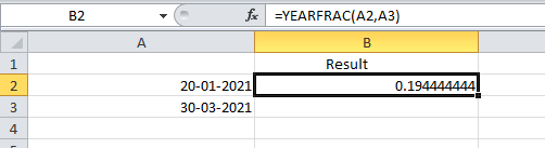
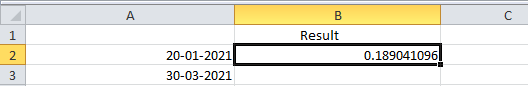
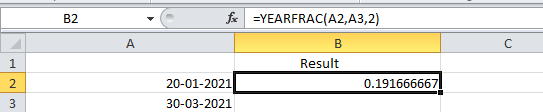
14. YEARFRAC Function
This function returns the fraction of the year which represents the number of whole days between the start & end date.
Syntax:
YEARFRAC(start_date,end_date,[basis])
Arguments:
1. start_date: This is the start date in the serial number.
2. end_date: This is the end date in the serial number.
3. basis: This is the optional argument that specifies the day count method.
| Basis | Day count method |
|---|---|
| 0(default) | US 30/360 |
| 1 | actual/actual |
| 2 | actual/360 |
| 3 | actual/365 |
| 4 | European 30/360 |
Example 1:
Using someday count methods.
Example 2:
Example 3:
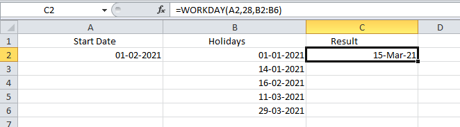
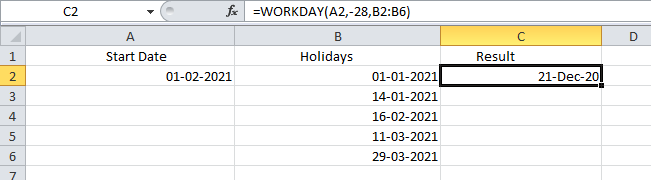
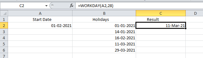
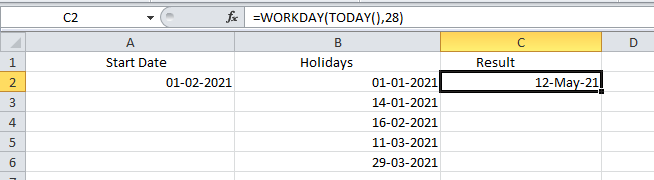
15. WORKDAY Function
This function helps if we exactly know how many working days we have & want to find out the date when the number of working will skip. This function always includes working days & excludes weekend days.
Syntax:
WORKDAY(start_date,days,holidays)
Arguments:
1. start_date: This argument is the date from which the counting of weekdays begins. Excel doesn’t include start_date as a working day.
2. days: This is the number of working days.
3. holidays: This is an optional argument. If the days mentioned include any holidays, then we need to make a list of holidays separately for this, and mention it here.
Example 1:
28 workdays from the start date, excluding holidays.
Example 2:
28 workdays before the start date, excluding holidays
Example 3:
28 workdays from the start date, no holidays.
Example 4:
28 workdays from today’s date, no holidays.
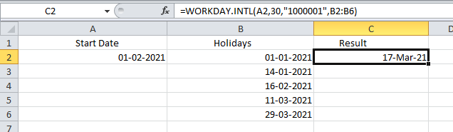
16. WORKDAY.INTL Function
This is a modification of the WORKDAY function as it provides a custom weekend parameter that distinguishes this from the WORKDAY function.
Syntax:
WORKDAY.INTL(start_date,days,[weekends],holidays)
Arguments:
1. start_date: This argument is the date from which the counting of weekdays begins. Excel doesn’t include start_date as a working day.
2. days: This is the number of working days.
3. holidays: This is an optional argument. If the days mentioned include any holidays, then we need to make a list of holidays separately for this and mention it here.
4. weekends: Through this argument, we can specify which days of the week to be treated as non-working days, either by weekend number or specific character string.
Weekend Number:
| Numbers | Days |
|---|---|
| 1 (default) | Saturday, Sunday |
| 2 | Sunday, Monday |
| 3 | Monday, Tuesday |
| 4 | Tuesday, Wednesday |
| 5 | Wednesday, Thursday |
| 6 | Thursday, Friday |
| 7 | Friday, Saturday |
| 11 | Sunday |
| 12 | Monday |
| 13 | Tuesday |
| 14 | Wednesday |
| 15 | Thursday |
| 16 | Friday |
| 17 | Saturday |
If this weekend argument is blank in this function, then it will automatically take the combination of Saturday & Sunday.
For instance:
- “0000011”-Saturday & Sunday are weekends(non-working days)
- “1000010”-Monday & Saturday are weekends(non-working days)
Example 1:
30 days from the start date, excluding holidays & Sunday, and Monday as weekends (by giving weekend number 2 as arguments).
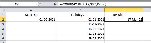
Example 2:
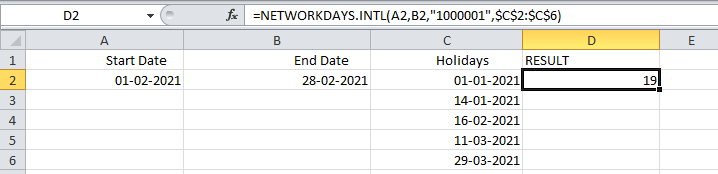
30 days from the start date, excluding holidays & Sunday, Monday as weekends(by giving weekend string “1000001” as arguments).
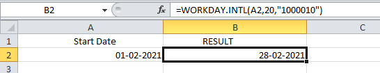
Example 3:
20 days from the start date, no holidays & Monday, Saturday as weekends (by giving weekend string “1000010” as arguments).
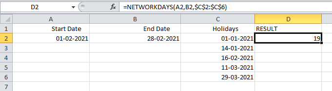
17. NETWORKDAYS Function
This function returns the number of working days between two dates, excluding weekends & holidays are as optional arguments.
Syntax:
NETWORKDAYS(start_date,end_date,holidays)
Arguments:
1. start_date: The initial date to start evaluation.
2. end_date: The last date to end the evaluation.
4. holidays: Used to specify holidays.
Example 1:
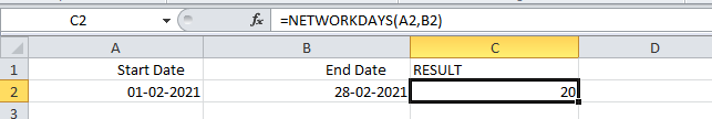
Example 2:
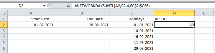
18. NETWORKDAYS.INTL Function
This function also returns the number of working days between two dates but provides the additional argument weekend to specify which days should be counted as weekend days.
The structure of the weekend argument is the same as for WORKDAY.INTL i.e. we can use either the weekend number or character string.
Syntax:
NETWORKDAYS.INTL(start_date,end_date,[weekend],holidays)
Arguments:
1. start_date: The initial date to start the evaluation.
2. end_date: The last date to end the evaluation.
3. weekend: Use to specify the weekends.
4. holidays: Used to specify holidays.
Example 1:
Here, the weekend argument is given in the form of a number.
Example 2:
Here, the weekend argument is given in the form of a character string of 0’s & 1’s.
Hopefully, this extensive overview of Excel’s date functions has given you a general idea of how date formulas in Excel operate. I advise you to read more articles on Excel if you want to understand more. I appreciate your time and look forward to hearing from you soon!
FAQs on DATE Functions in Excel
Here are some of the most frequently asked questions on DATE Functions in Excel
1. What is a Date function?
The DATE function in Excel combines the three independent values of year, month, and day to create a date.
Syntax: DATE(year,month,day)
2. How do I get DD MMM YYYY in Excel?
- Pick the cell that contain the date>right-click and select Format Cells
- Select Custom in the Number Tab>type ‘dd-mmm-yyyy’ in the Type text box>click OK.
The DATE function is a financial analyst’s best pal and categorized as a Date/Time function in Excel. The criticality of the DATE function’s role is sourced from Excel’s reluctance to keep the day, month, and year as a date. Instead, Excel stores them as a serial number.
Directly handing over dates as a text string may not work well for all Excel functions. So, we will supply the dates as a serial number using the DATE function to ensure that Excel and our worksheet formulas understand the instructions properly.

Syntax
The syntax of Excel Date function is as follows:
=DATE(year, month, day)
Arguments:
year – This is a required argument that represents the year component in the date. Enter it as a 4 digit number; entering a single digit will result in Excel automatically adding 1900 to it.
For example, entering year as ’10’ will instruct the formula to interpret the year argument as ‘1910’.
Excel refers to your computer’s date system set up to interpret the Year argument. Note that entering a negative value or a value greater than 9999 will return a #NUM! error.
month – This is a required argument that represents the month component in the date. Ideally, it must be an integer from 1 to 12 (January to December).
Alternatively, if you input a number greater than 12, Excel will count that many months starting from January of the year specified in the year argument. For example, entering year as 2001 and month as 18 will return a serial number that represents June 01, 2002. Note that Excel will return the date as the first date of the interpreted month (June 01 in our case), regardless of what you input in the date argument.
On the other hand, if you enter a value less than 1, Excel will reduce that many months from January of the year specified, plus 1. For example, if you enter month as -10 and year as 2001, Excel will return a serial number that represents February 01, 2000.
day – This is a required argument that represents the day component of the date. While in an ideal case, you will enter an integer from 1 to 31 as the date argument, it can be supplied as any other positive or negative integer and Excel will apply the same principles to compute the date as it does for the month argument.
Important characteristics of the DATE function
- DATE function returns a #NUM! error when
yearargument is supplied with a negative number or a number greater than 9999. - DATE function returns a #VALUE! error when any of its three arguments is supplied with a non-numeric value.
- If you see the Excel DATE function is returning a serial number like 36557 instead of a date, you will need to change the cell’s format. To do this, select the cell containing the returned date and search for the ‘Short Date’ option in the drop-down menu of cell formatting options in the ‘Number group’. These options sit on Excel’s Home Tab that appears at the top left.
Examples of the DATE function
Now let’s have a look at some of the examples of the DATE function in Excel.
Example 1 – The Plain – Vanilla DATE formula
In its purest form, this is what a DATE formula looks like:
=DATE(2001, 3, 15)

This formula returns a serial number that corresponds to the date March 15, 2001.
However, the formula can be slightly tweaked to incorporate the TODAY function encapsulated inside the YEAR function in Excel as well, like so:
=DATE(YEAR(TODAY()), 3, 15)

This formula will fetch the serial number for the current year (and the specified month and day), and return 03/15/2021.
Much the same way, you can use the TODAY function for the month argument as well, like so:
=DATE(YEAR(TODAY()), MONTH(TODAY()), 15)

This formula will fetch the serial number for the current year as well as the current month (and the specified day), and return 02/15/2021.
Example 2 – Using Cell References in DATE function Arguments
If the values you want to supply in the arguments are stored in cells on your spreadsheet, you can reference those cells, like so:
=DATE(A2, B2, C2)

With the values supplied from column A, the DATE function returns 04/30/2001.
Example 3 – Converting a number into a date using the DATE function
Let’s say you scalped the internet and landed on a large data set with dates written in a format that Excel does not understand (for example, 20052005).
In that (or similar) case, we can use the following formula to help Excel make sense of the data and interpret these numbers appropriately as dates:
=DATE(RIGHT(A2, 4), MID(A2, 3, 2), LEFT(A2, 2))

Recommended Reading: Excel MID Function
Addition and Subtraction of Dates With DATE function
We discussed earlier how Excel store dates as serial numbers. There is of course a logical reason why Excel does this – it enables us to add or subtract a specified number of days from a given date.
To illustrate how this works, we plugged the following formula into our sheet:
=DATE(2001, 3, 15) + 20

When you add a +20 at the end of this DATE formula, Excel will return the date 20 days after 03/15/2001, which is 04/04/2001.
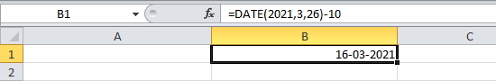
Alternatively, to subtract a certain number of days, all you need to do is use a minus sign, like so:
=DATE(2001, 3, 15) - 10

But, let’s say you want to compute the number of days between today and another date. In that case, we will subtract both dates, like so:
=TODAY() - DATE(2021, 2, 20)

The formula will return the number of days between today (whenever that may be) and March 15, 2001.
Changing DATE format With DATE function
So, you added some neat formulas to your Excel sheet and everything worked out fine. But, let’s say you want to use different separators for the days (for example, ‘/’ instead of ‘-‘), or you want to use the name of the month instead of a number (for example, January instead of 01).
We discussed earlier that Excel will refer to your computer’s date format and uses the same format for displaying dates in a worksheet.
To change this format, you do not need a formula. Instead, you need to tweak some settings.
Select the cell that contains the output from the DATE function. Right-click, and choose «Format Cells». You should see the following dialogue box:

Choose the format of your preference and click «OK».
Conditional Formatting with DATE function
Let’s say you have a large data set and you want to separate the data points occurring before and after a certain date.
To do this, we will use Excel’s conditional formatting rules and instruct Excel to shade these 2 cells with 2 separate colors so it becomes easy for us to discern.
We have our dates listed out in column A, and we want to shade the dates occurring before 12/31/2012 in green, and the ones occurring after in red.
To illustrate the entire process, we will use the following formula as a starting point:
=$A2 < DATE(2012, 12, 31)

Notice how this formula returns a Boolean value but does not shade any cells.
Let’s move a step further and apply a shade.
Select the range A2:A8 and navigate to the «Conditional Formatting» drop-down menu in the «Styles» group under the «Home» tab, and select «Manage Rules»:

On the «Conditional Formatting Rules Manager» click the «New Rule» button.

After clicking on the «New Rule» you will see a list of Rule Types. Scroll over to «Use a formula to determine which cells to format» and choosing it will reveal a formula box. In this box, plug in the formula we used to fetch Boolean values and select the desired formatting, like so:

Click «OK» and you should return to the Conditional Formatting Rules Manager dialog box.
To shade the dates occurring after 12/21/2012 red, we will add another rule following the same process. The only difference, obviously, will be in the formula. Instead of using a ‘<‘, we will use a ‘>=’, like so: =$A2>=DATE(2012,12,31)

This is what the Rules Manager box should look like at this point. Make sure that the «Applies to» box contains the appropriate range.

As your final step, click on «Apply» and watch your date list switch colors.

I hope the guide gives you a confidence boost the next time you use DATE formulas in your worksheet. Remember, practice is key. By the time you are done practicing, we will have another Excel function for you to explore.