Excel date month extract

Given a date value in Excel, is it possible to extract the month name?

For example, given the 2020-04-23 can you return the value April?

Yes, of course you can! Excel can do it all.

In this post you’ll learn 8 ways you can get the month name from a date value.

Long Date Format

You can get the month name by formatting your dates!

Good news, this is super easy to do!

Format your dates:

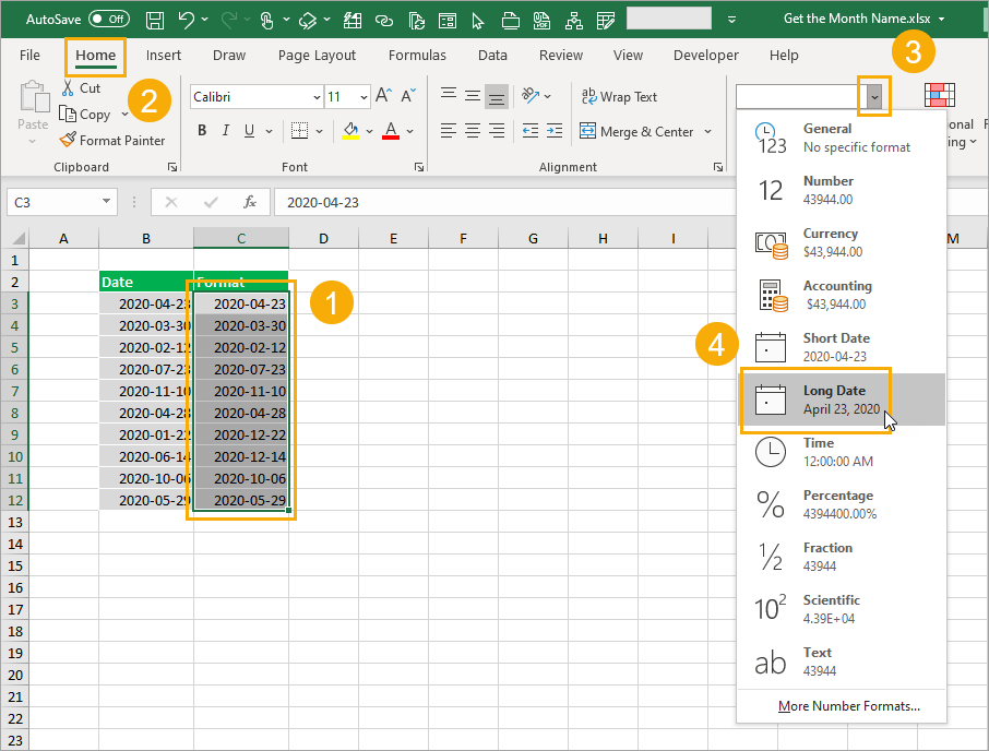
1. Select the dates you want to format.
2. Go to the Home tab in the ribbon commands.
3. Click on the drop-down in the Numbers section.
4. Select the Long Date option from the menu.

This will format the date 2020-04-23 as April 23, 2020, so you’ll be able to see the full English month name.

This doesn’t change the underlying value in the cell. It is still the same date, just formatted differently.

Custom Formats

This method is very similar to the long date format, but will allow you to format the dates to only show the month name and not include any day or year information.

Select the cells you want to format ➜ right click ➜ select Format Cells from the menu. You can also use the Ctrl + 1 keyboard shortcut to format cells.

In the Format Cells dialog box.

1. Go to the Number tab.
2. Select Custom from the Category options.
3. Enter mmmm into the Type input box.
4. Press the OK button.

This will format the date 2020-04-23 as April, so you’ll only see the full month name with no day or year part.

Again, this formatting won’t change the underlying value, it will just appear differently in the grid.

You can also use the mmm custom format to produce an abbreviated month name from the date such as Apr instead of April.

Flash Fill

Once you’ve formatted a column of date values in the long date format shown above, you’ll be able extract the name into a text value using flash fill.

Start typing a couple examples of the month name in the adjacent column to the formatted dates.

Excel will guess the pattern and fill its guess in a light grey. You can then press Enter to accept these values.

This way the month names will exist as text values and not just formatted dates.

TEXT Function

The previous formatting methods only changed the appearance of the date to show the month name.

With the TEXT function, you’ll be able to convert the date into a text value.

= TEXT ( B3, "mmmm" )

The above formula will take the date value in cell B3 and apply the mmmm custom formatting. The result will be a text value of the month name.

MONTH Functions

Excel has a MONTH function which can extract the month from a date.

MONTH and SWITCH

This is extracted as a numerical value from 1 to 12, so you will also need to convert that number into a name somehow. To do this you can use the SWITCH function.

= SWITCH (
    MONTH(B3),
    1,"January",
    2,"February",
    3,"March",
    4,"April",
    5,"May",
    6,"June",
    7,"July",
    8,"August",
    9,"September",
    10,"October",
    11,"November",
    12,"December"
)

The above formula is going to get the month number from the date in cell B3 using the MONTH function.

The SWITCH function will then convert that number into a name.

MONTH and CHOOSE

There’s an even more simple way to use the MONTH function as Wayne pointed out in the comments.

You can use the CHOOSE function since the month numbers can correspond to the choices of the CHOOSE function.

= CHOOSE (
    MONTH(B3),
    "January",
    "February",
    "March",
    "April",
    "May",
    "June",
    "July",
    "August",
    "September",
    "October",
    "November",
    "December"
)

The above formula is will get the month number from the date in cell B3 using the MONTH function, CHOOSE then returns the corresponding month name based on the number.

Power Query

You can also use power query to transform your dates into names.

First you will need to convert your data into an Excel table.

Then you can select your table and go to the Data tab and use the From Table/Range command.

This will open up the power query editor where you’ll be able to apply various transformation to your data.

Transform the date column to a month name.

1. Select the column of dates to transform.
2. Go to the Transform tab in the ribbon commands of the power query editor.
3. Click on the Date button in the Date & Time Column section.
4. Choose Month from the Menu.
5. Choose Name of Month from the sub-menu.

This will transform your column of dates into a text value of the full month name.

= Table.TransformColumns ( #"Changed Type", {{"Date", each Date.MonthName(_), type text}} )

This will automatically create the above M code formula for you and your dates will have been transformed.

You can then go to the Home tab and press Close & Load to load the transformed data back into a table in the Excel workbook.

Pivot Table Values

If you have dates in your data and you want to summarize your data by month, then pivot tables are the perfect option.

Select your data then go to the Insert tab and click on the Pivot Table command. You can then choose the sheet and cell to add the pivot table into.

Once you have your pivot table created, you will need to add fields into the Rows and Values area in the PivotTable Fields window.

Drag and drop the Date field into the Rows area and the Sales field into the Values area.

This will automatically create a Months field that summarizes the sales by month in you pivot table and the abbreviated month name will appear in your pivot table.

Power Pivot Calculated Column

You can also create calculated columns with pivot tables and the data model.

This will calculate a value for each row of data and create a new field for use in the PivotTable Fields list.

Follow the same steps as above to insert a pivot table.

In the Create Pivot Table dialog box, check the option to Add this data to the Data Model and press the OK button.

After creating the pivot table, go to the Data tab and press the Manage Data Model command to open the power pivot editor.

= FORMAT ( Table1[Date], "mmmm" )

Create a new column with the above formula inside the power pivot editor.

Close the editor and your new column will be available for use in the PivotTable Fields list.

This calculated column will show up as a new field inside the PivotTable Fields window and you can use it just like any other field in your data.

Conclusions

That’s 8 easy ways to get the month name from a date in Excel.

If you just want to display the name, then the formatting options might be enough.

Otherwise, you can convert the dates into names with flash fill, formulas, power query or even inside a pivot table.

What is your favourite method?

Dates are an important part of data. There are a few times when we need to use only a part from a date. Take an example of the month. Sometimes you only need a month from a date.

A month is one of the useful components of a date that you can use to summarize data and when it comes to Excel we have different methods to get a month from a date.

I’ve found a total of 5 methods for this. And today, in this post, I’d like to share with you all these methods to get/extract a month from a date. So let’s get down to the business.

1. MONTH Function

Using the MONTH function is the easiest method to extract a month from a date. All you need to do is just refer to a valid date in this function and it will return the number of the month ranging from 1 to 12.

=MONTH(A2)

You can also insert a date directly into the function using the correct date format.

Pro	Con
It’s easy to apply and there is no need to combine it with other functions.	Month number has limited use, most of the time it’s better to present the month name instead of numbers and if you want the month name then you need a different method.

2. TEXT Function

As I said, it’s better to use a month name instead of a month number. Using the TEXT function is a perfect method to extract the month name from a date. The basic work of the text function here is to convert a date into a month by using a specific format.

=TEXT(A2,"MMM")

By default, you have 5 different date formats which you can use in the text function. These formats will return the month name as a text. All you need to do is refer to a date in the function and specify a format. Yes, that’s all. And, make sure the date you are using should be a valid date as per Excel’s date system.

Pros	Cons
You have the flexibility to choose a format among 5 different formats and the original date column will remain the same.	It will return the month name which will be a text and using a custom abbreviation for the month name is not possible.

3. CHOOSE Function

Let’s say you want to get a custom month name or maybe a name in a different language instead of a number or a normal name. In that situation, CHOOSE function can help you. You need to specify a custom name for all 12 months in the function and need to use the month function to get the month number from the date.

=CHOOSE(MONTH(A1),"Jan","Feb","Mar","Apr","May","Jun","Jul","Aug","Sep","Oct","Nov","Dec")

When the month function returns a month number from the date, choose function will return the custom month name instead of that number.

Related: Formula Bar

Pros	Cons
It allows you more flexibility and you can specify a custom month name for each month.	It’s a time-consuming process to add all the values in the function one by one.

4. Power Query

If you want to get a month’s name from a date in a smart way then power query is your calling. It can allow you to convert a date into a month and extract a month number or a month name from a date as well. Power Query is a complete package for you to work with dates. Here you have the below data and here you need months from dates.

• First of all, convert your data into a table.
• After that, select any of the cells from the table and go to the data tab.
• From the data tab, click on “From Table”.

• It will load your table in the power query editor.

From here, you have two different options one is to add a new column with the month name or month number or convert your dates into a month name or month number. Skip the next two steps if you just want to convert your dates into months without adding a new column.

• First of all, right-click on the column heading.
• And after that, click “Duplicate Column”.

• Select the new column from the heading and right-click on it.
• Go to Transform ➜ Month ➜ Name of Month or Month.

• It will instantly convert dates into months.

• Just one more thing, right-click on the column heading and rename the column to “Month”.
• In the end, click on “Close & Load” and it will load your data into a worksheet.

Pro	Con
It’s a dynamic and one-time set-up. Your original data will not get impacted.	You should have a power query in your Excel version and the name of the month will be as a full name.

5. Custom Formatting

If you don’t want to get into any formula method, the simple way you can use it to convert a date into a month is by applying custom formatting. Follow these simple steps.

1. Select the range of cells or the column.
2. Press the shortcut key Ctrl + 1.
3. From the format option, go to “Custom”.
4. Now, in the “Type” input bar enter “MM”, “MMM”, or “MMMMMM”.
5. Click OK.

Pros	Cons
It’s easy to apply and doesn’t change the date but its format.	As the value is a date, when you copy and paste it somewhere else as a value it will be a date, not text. If someone changes the format, the month’s name will be lost.

Conclusion

All the above methods can be used in different situations. But some of them are more frequently used.

TEXT function is applicable in most situations. On the other hand, you also have a power query to get months in a few clicks. If you ask me, I use the text function but these days I am more in love with power query so I would also like to use it.

In the end, I just want to say, you can use any of these methods according to your need. But you need to tell me one thing.

Which one is your favorite method?

Please share with me in the comment section, I’d love to hear from you. And, don’t forget to share this with your friends.

This post will guide you how to extract month and year from a date in excel. How do I get month and year from date cells  with a formula in Excel. How to convert date to month and year in Excel.

---

If you want to extract month and year from a date in Cell, you can use a formula based on the TEXT function.
Assuming that you have a list of data in range B1:B4 that contain dates, and you want to convert the normal excel date into year and month format (yyyymm), How to achieve it. You can use the following format:

=TEXT(B1,"yyyymm")

Type this formula into a blank cell and then press Enter key in your keyboard. and drag the AutoFill Handle over other cells to apply this formul.

This formula will get a date with the year and month only from the orignial date in Cells.

If you only want to extract month from a date, and you can use the following formula:

=TEXT(B1,"mmm")

If you want to convert date to year format only, you can use the following formula:

=TEXT(B1,"yyyy")

 

---

• Excel Text function
  The Excel TEXT function converts a numeric value into text string with a specified format. The TEXT function is a build-in function in Microsoft Excel and it is categorized as a Text Function. The syntax of the TEXT function is as below: = TEXT (value, Format code)…

How to Use Excel > Excel Formula > How to Extract Day, Month and Year from Date in Excel

How to Extract Day, Month and Year from Date in Excel

Table of contents :

• Extract Day from Date in Excel
• Extract Month from Date in Excel
• Extract Year from Date in Excel

Excel provides three different functions to extract a day, month, and year from date. The following is an explanation of each function to extract each value.

Extract Day from Date in Excel

The formula

=DAY(A2)

The result

If you want to extract the day from the date, you can use the DAY function. The DAY function requires only one argument, fill it with valid excel date value.

The result, there are four days value and one error #VALUE!. An error occurred because 2/29/2006 is not a valid Excel date value. Why? Because 2006 is not a leap year, so there is no February 29th.

The DAY function result is a number between 1 and 31.

Extract Month from Date in Excel

The formula

=MONTH(A2)

The result

To extract month from the date you need the MONTH function. Like the DAY function, the MONTH function has only one argument, filled with a valid Excel date value.

There is a #VALUE error. The error appearance is the same place as the #VALUE error in DAY function result. The cause of the error is the same; the date value in cell A5 is not a valid Excel date value. This error will still appear in all excel functions related to the date.

The MONTH function result is a number between 1 and 12.

Extract Year from Date in Excel

The formula

=YEAR(A2)

The result

To extract the year from date, Excel provides the YEAR function. There is an argument that must be filled with a valid Excel date value.

The results of the DAY and MONTH functions are a number with a narrow range. Instead, the YEAR function is a wide range of numbers between 1900 and 9999.

For years less than 1900 or more than 9999, it will be considered an invalid excel date value. If used by an Excel function (related to the date function) returns a #VALUE! Error.

The DAY, MONTH and YEAR functions extract day, month and year from a date. To do the opposite, converting day, month and year in number to date value, you need the DATE function.

Related Function

Function used in this article

With endless streams of data, we keep bouncing back to the same thing; organizing. Because data needs to be discernable and that requires displaying or sorting data differently. Dates may need to be split into days, months, or years for the associated analysis and we’re focusing on one chunk of that for now.

In this tutorial, you will see a few ways on how to extract and display the month from a full date. Those ways use the TEXT, MONTH, CHOOSE and SWITCH functions and a custom date format. The methods are simple and explained thoroughly and you can pick one as per your Excel state of affairs.

Your options are the month in text (e.g. January, Jan, or custom), number (1 or 01), or display form (with the date value still intact). Therefore…..

Let’s get extracting! (No pain dental or otherwise.)

Using TEXT Function

The first method is simple, plain, and effective and is overlooked by the TEXT function. This function can be used to extract the month from a date in Excel. The TEXT function takes a value and converts it to text in the given number format. As to why we’re talking about a value being text and a number format in the same go, you’ll see in a while how the two meld together.

In this tutorial, we will use an example of the start and completion dates of writing a children’s book series. As a once-over, it would be helpful seeing what months the dates fall on. See this formula below and use it to extract the month from a full date using the TEXT function:

=TEXT(C3,"mmmm")

The TEXT function here is using the date in C3 and the format for the text is given by us as “mmmm”. This is the format code for the full month name. We have copied the formula down and across for the start and completion dates; these are the results for us:

In the formula, apply a different number format code enclosed in double quotes for the preferred output:

• m – returns the month number in a single digit (1 for January and 12 for December).
• mm – returns the month number in double digits (01 for January and 12 for December).
• mmm – returns the initial 3 letters of the month name (Jan for January and Dec for December).
• mmmm – returns the month name in full (January for January).

Bonus: Calendar/Fiscal Quarters

Where would we be without a small Excel trick in the balance? Out of balance? Keeping all in equilibrium, this is a little detail you can add to the data; the quarter of the year the month falls in. Use a formula like so to attach the related quarter with the month extracted from the date:

=TEXT(C3,"mmmm")&" Quarter "&ROUNDUP(MONTH(C3)/3,0)

The first part of the formula is the TEXT function, picked straight out as it was used earlier. The second part is the text «Quarter» added with a leading and trailing space by the & operator.

The third part, also joined using the & operator, is the quarter number calculated by the MONTH and ROUNDUP functions. The MONTH function takes the month from the date in C3, i.e. 1. In the formula, we divide this number by 3 (1/3 equals 0.33) and use the ROUNDUP function to round the resulting number up to the nearest integer (0.33 rounds up to the number 1).

This number defines what quarter the month in the date falls in. That completes the formula and all the results are shown here:

Now you can see that the month function should be quite useful in this tutorial, and it is. We’ll explore a few more ways with the MONTH function for extracting months from dates. Let’s go into what the function itself can do.

Recommended Reading: How to Extract Year from Date

Using MONTH Function

In the preceding section, the month name was returned. Now this method we’re about to see returns the number of the month instead of the month name from a date. This is done with the MONTH function in Excel. The MONTH function on its own picks the month from a date and results in the month number (from 1 to 12, sequentially for the 12 months).

With this simple formula, you can get the month number from the date in C3:

=MONTH(C3)

The MONTH function will only need a date to sift out the month and return the month number:

Using MONTH Function with CHOOSE

Life comes with many difficult decisions and sometimes making a choice is the hardest thing. But in Excel, when you have it all mapped out, the CHOOSE function has it all figured out. The CHOOSE function takes an index number and returns a value set against that number. Therefore, it can be incorporated with the MONTH function to extract the month from a date and then return the month name.

Hold on, haven’t we done that already? And the CHOOSE function would also require listing all the twelve values down so why is it even useful here when there are simpler ways and shorter formulas to get the month name?

Suppose we want to assign codes to our book collection and a part of that code is 2 letters of the start month and 2 letters of the completion month, we would want the month names from the dates in 2 letters. So, we’ll abbreviate the month names (e.g. Jr for January, Fb for February) and use the following formula:

=CHOOSE(MONTH(C3),"Jr","Fb","Mr","Ap","My","Jn","Jl","Ag","Sp","Oc","Nv","Dc")

All the abbreviated month names have been typed out in order in the formula. This readies the CHOOSE function to pick out the month and display it when it gets the index number. The index number is brought about by the MONTH function in our example case. the MONTH function takes C3’s date and picks the month out as 1. This index number is passed to the CHOOSE function and it returns the first value lined up in the formula i.e. Jr.

The formula goes on that way e.g. with the date in D8, the month number comes out as 10. Against the number 10, the value in the formula is Oc which is displayed in F8.

You know what that also means? It means that if you accidentally get the order of the months wrong, the results will be misleading and you wouldn’t even be aware. Excel gasp. There can be one way around this and it’s right around the corner. Actually it’s right ahead. Read below. 

Recommended Reading: How to Convert Date to Month and Year in Excel

Using MONTH Function with SWITCH

Now let’s switch things up a little. What a call that is, we are talking about the SWITCH function and how it can be used to pull the month from a date in Excel. Yes, we already know that can be done but what we’re trying to avoid here is the lineup problems that come with the CHOOSE function.

The SWITCH function, much like CHOOSE, evaluates a value (e.g. a3) against a list of values (from a1 to a12) and returns its corresponding value (returns b3 against a3). So the first yay with the SWITCH function is that the values can be placed in any order, unlike the CHOOSE function.

The second yay is that in case there’s no matching value, an added default value will be returned. The nay is that all the values and their corresponding values will have to be listed in the formula (though this may be a yay point where the values will not be as straightforward as 1, 2, 3 and will have to be defined anyway).

Here is how the formula rolls out with the SWITCH and MONTH functions for extracting months from dates:

=SWITCH(MONTH(C3),7,"Jl", 8,"Ag", 9,"Sp", 10,"Oc", 11,"Nv", 12,"Dc", 1,"Jr", 2,"Fb", 3,"Mr", 4,"Ap", 5,"My", 6,"Jn")

The difference from the CHOOSE function is quickly notable here; not only are the abbreviated months listed but also the values that they correspond to; the numbers. You can also see that the order is not important here as we have listed July first in the formula but what is important is getting the corresponding values right.

Again, the MONTH function will return the month number from the date in C3 and the SWITCH function will pull out the corresponding value from the formula and we will end up with “Jr” as the result.

Hence, the final upside of using the SWITCH or the CHOOSE function is that you can get either function to deliver custom values for the months. If this is not your requirement, go with the TEXT function. You can also have the cell display the month but still be usable as a date but you’re going to have to read ahead.

Using Custom Date Format

If your requirement isn’t as quirky as what you just saw, we have another way to get the month of a date to show. Use a Custom date format to make the name of the month appear instead of the date. If you’re okay with overwriting the data, use the format on the original data containing the dates. Otherwise, copy-paste the dates to the target column and apply the format there. The steps below will show you what to do to get the months from the dates after copy-pasting the dates to separate columns:

• Select the dates where you want the month names instead.
• Then click on the Number dialog launcher in the Home

• The Format Cells dialog box will open with the Number tab and you will see the current format of the selected cells.

• Click on the Custom category from the left panel. This will also show you the formatting code for the current format.

• Change the formatting code by entering the relevant format in the Type
• For the full month name, enter mmmm. For more formatting codes related to the month name and number, refer back to the earlier section on using the TEXT function.

• When done, click on the OK

The dates in the selected cells will be formatted to just the month names.

Note that the month names are only a display as the cells have been formatted. The original value is still the full date which can be confirmed by selecting any cell; you will see the date in the Formula Bar.

Since the original value is still a date, it can be used regularly in formulas and calculations as any date would.

We hope you’re Excel-updated on how to get the month from a date with some of the simple ways and Excel tricks shown in this tutorial. We also hope that this guide has pulled you into some sightseeing around here because if you look at it our way, Excel is a maze and we’re here with all the right cheat codes. You won’t get lost, give it a try!