
17 авг. 2022 г.
читать 2 мин
В этом руководстве объясняется, как преобразовать дату в число в трех различных сценариях:
1. Преобразуйте одну дату в число
2. Преобразуйте несколько дат в числа
3. Преобразование даты в количество дней с другой даты
Давайте прыгать!
Пример 1: преобразование одной даты в число
Предположим, мы хотим преобразовать дату «10.02.2022» в число в Excel.
Для этого мы можем использовать функцию ДАТАЗНАЧ в Excel:
=DATEVALUE("2/10/2022")
По умолчанию эта функция вычисляет количество дней между заданной датой и 01.01.1900 .
На следующем снимке экрана показано, как использовать эту функцию на практике:
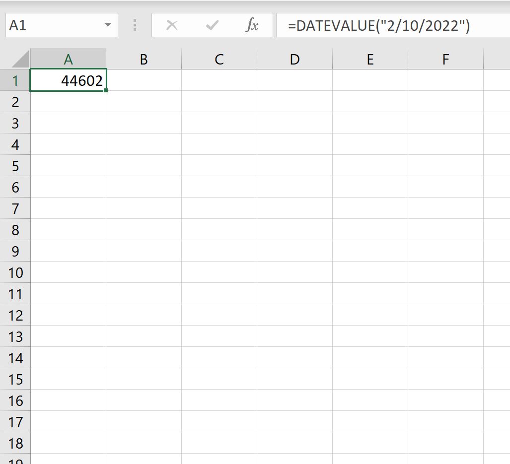
Это говорит нам о том, что между 10.02.2022 и 01.01.1900 существует разница в 44 602 дня.
Пример 2. Преобразование нескольких дат в числа
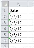
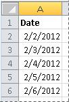
Предположим, у нас есть следующий список дат в Excel:

Чтобы преобразовать каждую из этих дат в число, мы можем выделить диапазон ячеек, содержащих даты, затем щелкнуть раскрывающееся меню «Числовой формат » на вкладке « Главная » и выбрать « Число »:

Это автоматически преобразует каждую дату в число, представляющее количество дней между каждой датой и 01.01.1900 :

Пример 3. Преобразование даты в количество дней, прошедших с другой даты
Мы можем использовать следующую формулу для преобразования даты в количество дней, прошедших с другой даты:
=DATEDIF( B2 , A2 , "d")
Эта конкретная формула вычисляет количество дней между датой в ячейке B2 и датой в ячейке A2 .
На следующем снимке экрана показано, как использовать формулу DATEDIF для расчета количества дней между датами в столбце A и 01.01.2022:

Вот как интерпретировать значения в столбце B:
- Между 01.01.2022 и 01.04.2022 есть 3 дня.
- Между 01.01.2022 и 01.01.2022 8 дней.
- Между 01.01.2022 и 15.01.2022 14 дней.
И так далее.
Дополнительные ресурсы
В следующих руководствах объясняется, как выполнять другие распространенные задачи в Excel:
Как автозаполнять даты в Excel
Как использовать СЧЁТЕСЛИМН с диапазоном дат в Excel
Как рассчитать среднее значение между двумя датами в Excel
Содержание
- DATEVALUE function
- Description
- Syntax
- Remarks
- Example
- Как преобразовать дату в число в Excel (3 примера)
- Пример 1: преобразование одной даты в число
- Пример 2. Преобразование нескольких дат в числа
- Пример 3. Преобразование даты в количество дней, прошедших с другой даты
- Дополнительные ресурсы
- Convert dates stored as text to dates
- Need more help?
- How to convert text to date and number to date in Excel
- How to distinguish normal Excel dates from «text dates»
- How to convert number to date in Excel
- How to convert 8-digit number to date in Excel
- How to convert text to date in Excel
- Excel DATEVALUE function — change text to date
- Excel DATEVALUE function — things to remember
- Excel VALUE function — convert a text string to date
- Mathematical operations to convert text to dates
- How to convert text strings with custom delimiters to dates
- Text to Columns wizard — formula-free way to covert text to date
- Example 1. Converting simple text strings to dates
- Example 2. Converting complex text strings to dates
- Quick conversion of text dates using Paste Special
- Fixing text dates with two-digit years
- How to turn on Error Checking in Excel
- How to change text to date in Excel an easy way
DATEVALUE function
This article describes the formula syntax and usage of the DATEVALUE function in Microsoft Excel.
Description
The DATEVALUE function converts a date that is stored as text to a serial number that Excel recognizes as a date. For example, the formula =DATEVALUE(«1/1/2008») returns 39448, the serial number of the date 1/1/2008. Remember, though, that your computer’s system date setting may cause the results of a DATEVALUE function to vary from this example
The DATEVALUE function is helpful in cases where a worksheet contains dates in a text format that you want to filter, sort, or format as dates, or use in date calculations.
To view a date serial number as a date, you must apply a date format to the cell. Find links to more information about displaying numbers as dates in the See Also section.
Syntax
The DATEVALUE function syntax has the following arguments:
Date_text Required. Text that represents a date in an Excel date format, or a reference to a cell that contains text that represents a date in an Excel date format. For example, «1/30/2008» or «30-Jan-2008» are text strings within quotation marks that represent dates.
Using the default date system in Microsoft Excel for Windows, the date_text argument must represent a date between January 1, 1900 and December 31, 9999. The DATEVALUE function returns the #VALUE! error value if the value of the date_text argument falls outside of this range.
If the year portion of the date_text argument is omitted, the DATEVALUE function uses the current year from your computer’s built-in clock. Time information in the date_text argument is ignored.
Excel stores dates as sequential serial numbers so that they can be used in calculations. By default, January 1, 1900 is serial number 1, and January 1, 2008 is serial number 39448 because it is 39,447 days after January 1, 1900.
Most functions automatically convert date values to serial numbers.
Example
Copy the example data in the following table, and paste it in cell A1 of a new Excel worksheet. For formulas to show results, select them, press F2, and then press Enter. If you need to, you can adjust the column widths to see all the data.
Источник
Как преобразовать дату в число в Excel (3 примера)

В этом руководстве объясняется, как преобразовать дату в число в трех различных сценариях:
1. Преобразуйте одну дату в число
2. Преобразуйте несколько дат в числа
3. Преобразование даты в количество дней с другой даты
Пример 1: преобразование одной даты в число
Предположим, мы хотим преобразовать дату «10.02.2022» в число в Excel.
Для этого мы можем использовать функцию ДАТАЗНАЧ в Excel:
По умолчанию эта функция вычисляет количество дней между заданной датой и 01.01.1900 .
На следующем снимке экрана показано, как использовать эту функцию на практике:
Это говорит нам о том, что между 10.02.2022 и 01.01.1900 существует разница в 44 602 дня.
Пример 2. Преобразование нескольких дат в числа
Предположим, у нас есть следующий список дат в Excel:
Чтобы преобразовать каждую из этих дат в число, мы можем выделить диапазон ячеек, содержащих даты, затем щелкнуть раскрывающееся меню «Числовой формат » на вкладке « Главная » и выбрать « Число »:
Это автоматически преобразует каждую дату в число, представляющее количество дней между каждой датой и 01.01.1900 :
Пример 3. Преобразование даты в количество дней, прошедших с другой даты
Мы можем использовать следующую формулу для преобразования даты в количество дней, прошедших с другой даты:
Эта конкретная формула вычисляет количество дней между датой в ячейке B2 и датой в ячейке A2 .
На следующем снимке экрана показано, как использовать формулу DATEDIF для расчета количества дней между датами в столбце A и 01.01.2022:
Вот как интерпретировать значения в столбце B:
- Между 01.01.2022 и 01.04.2022 есть 3 дня.
- Между 01.01.2022 и 01.01.2022 8 дней.
- Между 01.01.2022 и 15.01.2022 14 дней.
Дополнительные ресурсы
В следующих руководствах объясняется, как выполнять другие распространенные задачи в Excel:
Источник
Convert dates stored as text to dates
Occasionally, dates may become formatted and stored in cells as text. For example, you may have entered a date in a cell that was formatted as text, or the data might have been imported or pasted from an external data source as text.
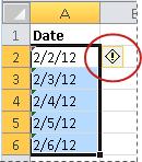
Dates that are formatted as text are left-aligned in a cell (instead of right-aligned). When Error Checking is enabled, text dates with two-digit years might also be marked with an error indicator:  .
.
Because Error Checking in Excel can identify text-formatted dates with two-digit years, you can use the automatic correction options to convert them to date-formatted dates. You can use the DATEVALUE function to convert most other types of text dates to dates.
If you import data into Excel from another source, or if you enter dates with two-digit years into cells that were previously formatted as text, you may see a small green triangle in the upper-left corner of the cell. This error indicator tells you that the date is stored as text, as shown in this example.
You can use the Error Indicator to convert dates from text to date format.
Notes: First, ensure that Error Checking is enabled in Excel. To do that:
Click File > Options > Formulas.
In Excel 2007, click the Microsoft Office button  , then click Excel Options > Formulas.
In Error Checking, check Enable background error checking. Any error that is found, will be marked with a triangle in the top-left corner of the cell.
Under Error checking rules, select Cells containing years represented as 2 digits.
Follow this procedure to convert the text-formatted date to a normal date:
On the worksheet, select any single cell or range of adjacent cells that has an error indicator in the upper-left corner. For more information, see Select cells, ranges, rows, or columns on a worksheet.
Tip: To cancel a selection of cells, click any cell on the worksheet.
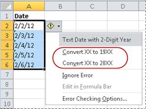
Click the error button that appears near the selected cell(s).
On the menu, click either Convert XX to 20XX or Convert XX to 19XX. If you want to dismiss the error indicator without converting the number, click Ignore Error.
The text dates with two-digit years convert to standard dates with four-digit years.
Once you have converted the cells from text-formatted dates, you can change the way the dates appear in the cells by applying date formatting.
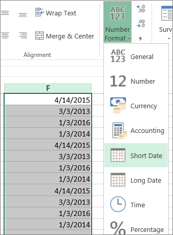
If your worksheet has dates that were perhaps imported or pasted that end up looking like a series of numbers like in the picture below, you probably would want to reformat them so they appear as either short or long dates. The date format will also be more useful if you want to filter, sort, or use it in date calculations.

Select the cell, cell range, or column that you want to reformat.
Click Number Format and pick the date format you want.
The Short Date format looks like this:
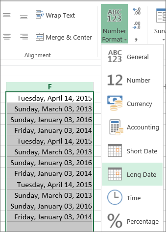
The Long Date includes more information like in this picture:
To convert a text date in a cell to a serial number, use the DATEVALUE function. Then copy the formula, select the cells that contain the text dates, and use Paste Special to apply a date format to them.
Follow these steps:
Select a blank cell and verify that its number format is General.
In the blank cell:
Click the cell that contains the text-formatted date that you want to convert.
Press ENTER, and the DATEVALUE function returns the serial number of the date that is represented by the text date.
What is an Excel serial number?
Excel stores dates as sequential serial numbers so that they can be used in calculations. By default, January 1, 1900, is serial number 1, and January 1, 2008, is serial number 39448 because it is 39,448 days after January 1, 1900.To copy the conversion formula into a range of contiguous cells, select the cell containing the formula that you entered, and then drag the fill handle  across a range of empty cells that matches in size the range of cells that contain text dates.
After you drag the fill handle, you should have a range of cells with serial numbers that corresponds to the range of cells that contain text dates.
Select the cell or range of cells that contains the serial numbers, and then on the Home tab, in the Clipboard group, click Copy.
Keyboard shortcut: You can also press CTRL+C.
Select the cell or range of cells that contains the text dates, and then on the Home tab, in the Clipboard group, click the arrow below Paste, and then click Paste Special.
In the Paste Special dialog box, under Paste, select Values, and then click OK.
On the Home tab, click the popup window launcher next to Number.
In the Category box, click Date, and then click the date format that you want in the Type list.
To delete the serial numbers after all of the dates are converted successfully, select the cells that contain them, and then press DELETE.
Need more help?
You can always ask an expert in the Excel Tech Community or get support in the Answers community.
Источник
How to convert text to date and number to date in Excel
 by Svetlana Cheusheva, updated on February 7, 2023
The tutorial explains how to use Excel functions to convert text to date and number to date, and how to turn text strings into dates in a non-formula way. You will also learn how to quickly change a number to date format.
Since Excel is not the only application you work with, sometimes you’ll find yourself working with dates imported in an Excel worksheet from a .csv file or another external source. When that happens, chances are the dates will export as text entries. Even though they look like dates, Excel won’t not recognize them as such.
There are many ways to convert text to date in Excel and this tutorial aims to cover them all, so that you can choose a text-to-date conversion technique most suitable for your data format and your preference for a formula or non-formula way.
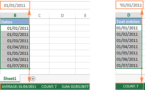
How to distinguish normal Excel dates from «text dates»
When importing data into Excel, there is often a problem with date formatting. The imported entries may look like normal Excel dates to you, but they don’t behave like dates. Microsoft Excel treats such entries as text, meaning you cannot sort your table by date properly, nor can you use those «text dates» in formulas, PivotTables, charts or any other Excel tool that recognizes dates.
There are a few signs that can help you determine whether a given entry is a date or a text value.
| Dates | Text values |
|
|
How to convert number to date in Excel
Since all Excel functions that change text to date return a number as a result, let’s have a closer look at converting numbers to dates first.
As you probably know, Excel stores dates and times as serial numbers and it is only a cell’s formatting that forces a number to be displayed as a date. For example, 1-Jan-1900 is stored as number 1, 2-Jan-1900 is stored as 2, and 1-Jan-2015 is stored as 42005. For more information on how Excel stores dates and times, please see Excel date format.
When calculating dates in Excel, the result returned by different date functions is often a serial number representing a date. For example, if =TODAY()+7 returns a number like 44286 instead of the date that is 7 days after today, that does not mean the formula is wrong. Simply, the cell format is set to General or Text while it should be Date.
To convert such serial number to date, all you have to do is change the cell number format. For this, simply pick Date in the Number Format box on the Home tab.
To apply a format other than default, then select the cells with serial numbers and press Ctrl+1 to open the Format Cells dialog. On the Number tab, choose Date, select the desired date format under Type and click OK. 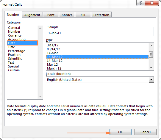
Yep, it’s that easy! If you want something more sophisticated than predefined Excel date formats, please see how to create a custom date format in Excel.
If some stubborn number refuses to change to a date, check out Excel date format not working — troubleshooting tips.
How to convert 8-digit number to date in Excel
It’s a very common situation when a date is input as an 8-digit number like 10032016, and you need to convert it into a date value that Excel can recognize (10/03/2016). In this case, simply changing the cell format to Date won’t work — you will get ########## as the result.
To convert such a number to date, you will have to use the DATE function in combination with RIGHT, LEFT and MID functions. Unfortunately, it is not possible to make a universal formula that will work in all scenarios because the original number can be input in a variety of different formats. For example:
| Number | Format | Date |
| 10032016 | ddmmyyyy | 10-Mar-2016 |
| 20160310 | yyyymmdd | |
| 20161003 | yyyyddmm |
Anyway, I will try to explain the general approach to converting such numbers to dates and provide a few formula examples.
For starters, remember the order of the Excel Date function arguments:
So, what you need to do is extract a year, month and date from the original number and supply them as the corresponding arguments to the Date function.
For example, let’s see how you can convert number 10032016 (stored in cell A1) to date 3/10/2016.
- Extract the year. It’s the last 4 digits, so we use the RIGHT function to pick the last 4 characters: RIGHT(A1, 4).
- Extract the month. It’s the 3 rd and 4 th digits, so we employ the MID function to get them MID(A1, 3, 2). Where 3 (second argument) is the start number, and 2 (third argument) is the number of characters to extract.
- Extract the day. It’s the first 2 digits, so we have the LEFT function to return the first 2 characters: LEFT(A2,2).
Finally, embed the above ingredients into the Date function, and you get a formula to convert number to date in Excel:
=DATE(RIGHT(A1,4), MID(A1,3,2), LEFT(A1,2))
The following screenshot demonstrates this and a couple more formulas in action: 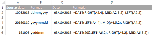
Please pay attention to the last formula in the above screenshot (row 6). The original number-date (161003) contains only 2 chars representing a year (16). So, to get the year of 2016, we concatenate 20 and 16 using the following formula: 20&LEFT(A6,2). If you don’t do this, the Date function will return 1916 by default, which is a bit weird as if Microsoft still lived in the 20 th century 🙂
Note. The formulas demonstrated in this example work correctly as long as all numbers you want to convert to dates follow the same pattern.
How to convert text to date in Excel
When you spot text dates in your Excel file, most likely you would want to convert those text strings to normal Excel dates so that you can refer to them in your formulas to perform various calculations. And as is often the case in Excel, there are a few ways to tackle the task.
Excel DATEVALUE function — change text to date
The DATEVALUE function in Excel converts a date in the text format to a serial number that Excel recognizes as a date.
The syntax of Excel’s DATEVALUE is very straightforward:
So, the formula to convert a text value to date is as simple as =DATEVALUE(A1) , where A1 is a cell with a date stored as a text string.
Because the Excel DATEVALUE function converts a text date to a serial number, you will have to make that number look like a date by applying the Date format to it, as we discussed a moment ago.
The following screenshots demonstrates a few Excel DATEVALUE formulas in action: 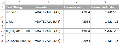
Excel DATEVALUE function — things to remember
When converting a text string to a date using the DATEVALUE function, please keep in mind that:
- Time information in text strings is ignored, as you can see in rows 6 and 8 above. To convert text values containing both dates and times, use the VALUE function.
- If the year is omitted in a text date, Excel’s DATEVALUE will pick the current year from your computer’s system clock, as demonstrated in row 4 above.
- Since Microsoft Excel stores dates since January 1, 1900 , the use of the Excel DATEVALUE function on earlier dates will result in the #VALUE! error.
- The DATEVALUE function cannot convert a numeric value to date, nor can it process a text string that looks like a number, for that you will need to use the Excel VALUE function, and this is exactly what we are going to discuss next.
Excel VALUE function — convert a text string to date
Compared to DATEVALUE, the Excel VALUE function is more versatile. It can convert any text string that looks like a date or number into a number, which you can easily change to a date format of your choosing.
The syntax of the VALUE function is as follows:
Where text is a text string or reference to a cell containing the text you want to convert to number.
The Excel VALUE function can process both date and time, the latter is converted to a decimal portion, as you can see in row 6 in the following screenshot: 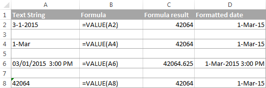
Mathematical operations to convert text to dates
Apart from using specific Excel functions such as VALUE and DATEVALUE, you can perform a simple mathematical operation to force Excel to do a text-to-date conversion for you. The required condition is that an operation should not change the date’s value (serial number). Sounds a bit tricky? The following examples will make things easy!
Assuming that your text date is in cell A1, you can use any of the following formulas, and then apply the Date format to the cell:
- Addition: =A1 + 0
- Multiplication: =A1 * 1
- Division: =A1 / 1
- Double negation: =—A1
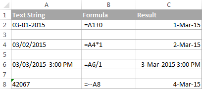
As you can see in the above screenshot, mathematical operations can convert dates (rows 2 and 4), times (row 6) as well as numbers formatted as text (row 8). Sometimes the result is even displayed as a date automatically, and you don’t have to bother about changing the cell format.
How to convert text strings with custom delimiters to dates
If your text dates contain some delimiter other than a forward slash (/) or dash (-), Excel functions won’t be able to recognize them as dates and return the #VALUE! error.
To fix this, you can run Excel’s Find and Replace tool to replace your delimiter with a slash (/), all in one go:
- Select all the text strings you want to convert to dates.
- Press Ctrl+H to open the Find and Replace dialog box.
- Enter your custom separator (a dot in this example) in the Find what field, and a slash in the Replace with
- Click the Replace All
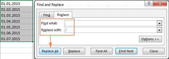
Now, the DATEVALUE or VALUE function should have no problem with converting the text strings to dates. In the same manner, you can fix dates containing any other delimiter, e.g. a space or a backward slash.
If you prefer a formula solution, you can use Excel’s SUBSTITUTE function instead of Replace All to switch your delimiters to slashes.
Assuming the text strings are in column A, a SUBSTITUTE formula may look as follows:
Where A1 is a text date and «.» is the delimiter your strings are separated with.
Now, let’s embed this SUBSTITUTE function into the VALUE formula:
And have the text strings converted to dates, all with a single formula. 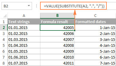
As you see, the Excel DATEVALUE and VALUE functions are quite powerful, but both have their limits. For example, if you are trying to convert complex text strings like Thursday, January 01, 2015, neither function could help. Luckily, there is a non-formula solution that can handle this task and the next section explains the detailed steps.
Text to Columns wizard — formula-free way to covert text to date
If you are a non-formula user type, a long-standing Excel feature called Text To Columns will come in handy. It can cope with simple text dates demonstrated in Example 1 as well as multi-part text strings shown in Example 2.
Example 1. Converting simple text strings to dates
If the text strings you want to convert to dates look like any of the following:
You don’t really need formulas, nor exporting or importing anything. All it takes is 5 quick steps.
In this example, we will be converting text strings like 01 01 2015 (day, month and year are separated with spaces) to dates.
- In your Excel worksheet, select a column of text entries you want to convert to dates.
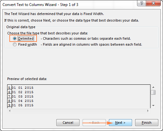
- Switch to the Data tab, Data Tools group, and click Text to Columns.

- In step 1 of the Convert Text to Columns Wizard, select Delimited and click Next.
- In step 2 of the wizard, uncheck all delimiter boxes and click Next.
- In the final step, select Date under Column data format, choose the format corresponding to your dates, and click Finish.

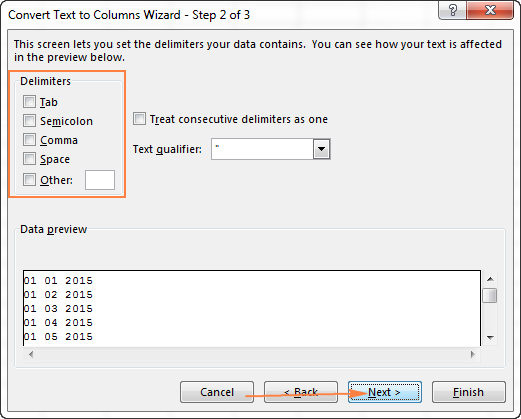
In this example, we are converting the text dates formatted as «01 02 2015» (month day year), so we select MDY from the drop down box. 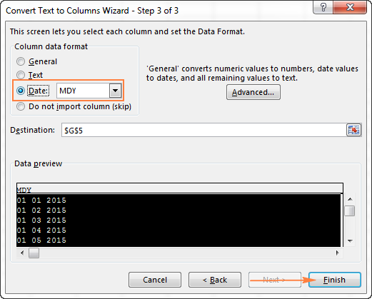
Now, Excel recognizes your text strings as dates, automatically converts them to your default date format and displays right-aligned in the cells. You can change the date format in the usual way via the Format Cells dialog.
Note. For the Text to Column wizard to work correctly, all of your text strings should be formatted identically. For example, if some of your entries are formatted like day/month/year format while others are month/day/year, you would get incorrect results.
Example 2. Converting complex text strings to dates
If your dates are represented by multi-part text strings, such as:
- Thursday, January 01, 2015
- January 01, 2015 3 PM
You will have to put a bit more effort and use both the Text to Columns wizard and Excel DATE function.
- Select all text strings to be converted to dates.
- Click the Text to Columns button on the Data tab, Data Tools group.
- On step 1 of the Convert Text to Columns Wizard, select Delimited and click Next.
- On step 2 of the wizard, select the delimiters your text strings contain.
For example, if you are converting strings separated by commas and spaces, like «Thursday, January 01, 2015″, you should choose both delimiters — Comma and Space. 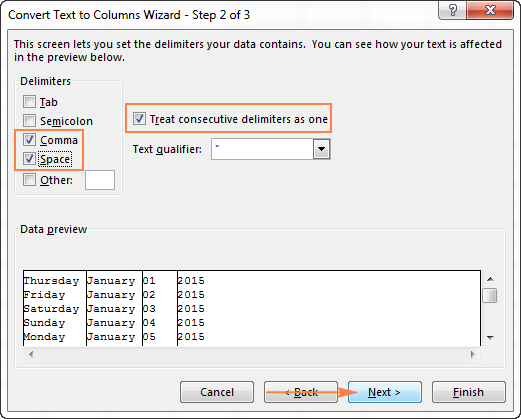
It also makes sense to select the «Treat consecutive delimiters as one» option to ignore extra spaces, if your data has any.
And finally, have a look at the Data preview window and verify if the text strings are split to columns correctly, then click Next.
On step 3 of the wizard, make sure all columns in the Data Preview section have the General format. If they don’t, click on a column and select General under the Column data format options.
Note. Do not choose the Date format for any column because each column contains only one component, so Excel won’t be able to understand this is a date.
If you don’t need some column, click on it and select Do not import column (skip).
If you don’t want to overwrite the original data, specify where the columns should be inserted — enter the address for the top left cell in the Destination field.
When done, click the Finish button. 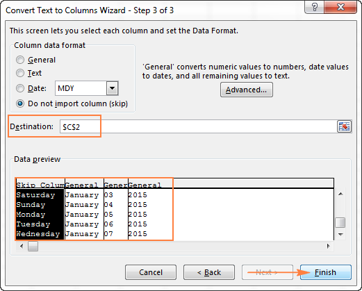
As you see in the screenshot above, we are skipping the first column with the days of the week, splitting the other data into 3 columns (in the General format) and inserting these columns beginning from cell C2.
The following screenshot shows the result, with the original data in column A and the split data in columns C, D and E.

Finally, you have to combine the date parts together by using a DATE formula. The syntax of the Excel DATE function is self-explanatory:
In our case, year is in column E and day is in column D, no problem with these.
It’s not so easy with month because it is text while the DATE function needs a number. Luckily, Microsoft Excel provides a special MONTH function that can change a month’s name to a month’s number:
For the MONTH function to understand it deals with a date, we put it like this:
Where C2 contains the name of the month, January in our case. «1&» is added to concatenate a date (1 January) so that the MONTH function can convert it to the corresponding month number.
And now, let’s embed the MONTH function into the month ; argument of our DATE formula:
And voila, our complex text strings are successfully converted to dates: 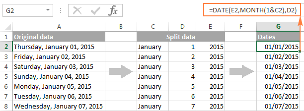
Quick conversion of text dates using Paste Special
To quickly convert a range of simple text strings to dates, you can use the following trick.
- Copy any empty cell (select it and press Ctrl + C ).
- Select the range with text values you want to convert to dates.
- Right-click the selection, click Paste Special, and select Add in the Paste Special dialog box:
- Click OK to complete the conversion and close the dialog.

What you have just done is tell Excel to add a zero (empty cell) to your text dates. To be able to do this, Excel converts a text string to a number, and since adding a zero does not change the value, you get exactly what you wanted — the date’s serial number. As usual, you change a number to the date format by using the Format Cells dialog.
To learn more about the Paste Special feature, please see How to use Paste Special in Excel.
Fixing text dates with two-digit years
The modern versions of Microsoft Excel are smart enough to spot some obvious errors in your data, or better say, what Excel considers an error. When this happens, you will see an error indicator (a small green triangle) in the upper-left corner of the cell and when you select the cell, an exclamation mark appears: 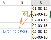
Clicking the exclamation mark will display a few options relevant to your data. In case of a 2-digit year, Excel will ask if you want to convert it to 19XX or 20XX.
If you have multiple entries of this type, you can fix them all in one fell swoop — select all the cells with errors, then click on the exclamation mark and select the appropriate option. 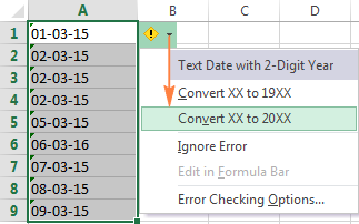
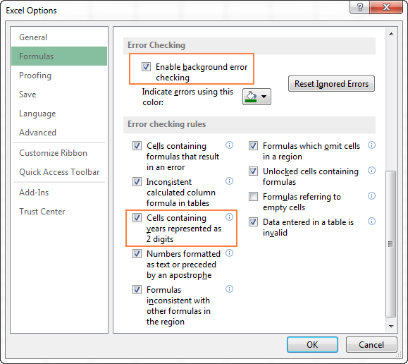
How to turn on Error Checking in Excel
Usually, Error Checking is enabled in Excel by default. To make sure, click File > Options > Formulas, scroll down to the Error Checking section and verify if the following options are checked:
- Enable background error checking under Error Checking;
- Cells containing years represented as 2 digits under Error checking rules.
How to change text to date in Excel an easy way
As you see, converting text to date in Excel is far from being a trivial one-click operation. If you are confused by all different use cases and formulas, let me show you a quick and straightforward way.
Install our Ultimate Suite (a free trial version can be downloaded here), switch to the Ablebits Tools tab (2 new tabs containing 70+ awesome tools will be added to your Excel!) and find the Text to Date button: 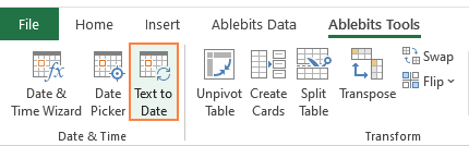
To convert text-dates to normal dates, here’s what you do:
- Select the cells with text strings and click the Text to Date button.
- Specify the date order (days, months and years) in the selected cells.
- Choose whether to include or not include time in the converted dates.
- Click Convert.
That’s it! The results of conversion will appear in the adjacent column, your source data will be preserved. If something goes wrong, you can simply delete the results and try again with a different date order. 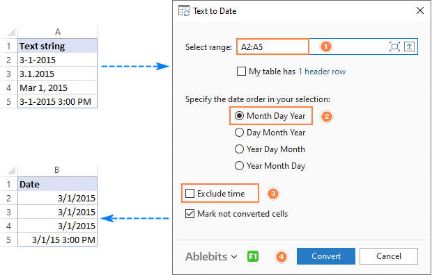
Tip. If you chose to convert times as well as dates, but the time units are missing in the results, be sure to apply a number format that shows both the date and time values. For more info, please see How to create custom date and time formats.
If you are curious to learn more about this wonderful tool, please check out its home page: Text to Date for Excel.
This is how you convert text to date in Excel and change dates to text. Hopefully, you have been able to find a technique to your liking. In the next article, we will tackle the opposite task and explore different ways of converting Excel dates to text strings. I thank you for reading and hope to see you next week.
Источник
This tutorial explains how to convert a date to a number in three different scenarios:
1. Convert One Date to Number
2. Convert Several Dates to Numbers
3. Convert Date to Number of Days Since Another Date
Let’s jump in!
Example 1: Convert One Date to Number
Suppose we would like to convert the date “2/10/2022” to a number in Excel.
We can use the DATEVALUE function in Excel to do so:
=DATEVALUE("2/10/2022")
By default, this function calculates the number of days between a given date and 1/1/1900.
The following screenshot shows how to use this function in practice:

This tells us that there is a difference of 44,602 days between 2/10/2022 and 1/1/1900.
Example 2: Convert Several Dates to Numbers
Suppose we have the following list of dates in Excel:

To convert each of these dates to a number, we can highlight the range of cells that contain the dates, then click the Number format dropdown menu on the Home tab and choose Number:

This will automatically convert each date to a number that represents the number of days between each date and 1/1/1900:

Example 3: Convert Date to Number of Days Since Another Date
We can use the following formula to convert a date to a number of days since another date:
=DATEDIF(B2, A2, "d")
This particular formula calculates the number of days between the date in cell B2 and the date in cell A2.
The following screenshot shows how to use the DATEDIF formula to calculate the number of days between the dates in column A and 1/1/2022:

Here’s how to interpret the values in column B:
- There are 3 days between 1/1/2022 and 1/4/2022.
- There are 8 days between 1/1/2022 and 1/9/2022.
- There are 14 days between 1/1/2022 and 1/15/2022.
And so on.
Additional Resources
The following tutorials explain how to perform other common tasks in Excel:
How to AutoFill Dates in Excel
How to Use COUNTIFS with a Date Range in Excel
How to Calculate Average If Between Two Dates in Excel
Return to Excel Formulas List
Download Example Workbook
Download the example workbook
This tutorial will demonstrate how to convert a date to a serial number corresponding to that date (or vis-a-versa) in Excel and Google Sheets
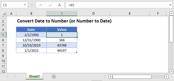
Date to Number
To convert a date to a serial number, all you need to do is change the formatting to General:
However, this won’t work if the date is stored as text.
Date Stored as Text to Number
If the date is stored as text, you can use DATEVALUE convert it to an Excel date:
=DATEVALUE(B3)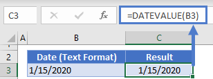
Then you can change the formatting to general to see the serial number.
Number to Date
To convert a serial number to a date, all you need to do is the change the formatting from General (or Number) to a date format (ex. Short Date):
Convert Date to Number in Google Sheets
All of the above examples work exactly the same in Google Sheets as in Excel.
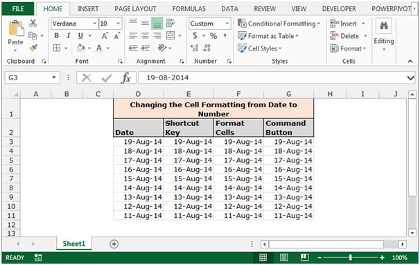
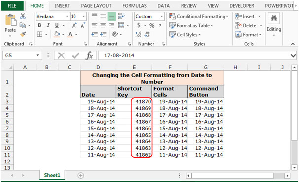
To change the cell format from date to number we convert the formatting into General Format in Microsoft Excel.
There are three different ways to change the formatting from date to number.
1st Shortcut Key
2nd Format Cells
3rd Command Button
Let’s take an example and understand how we can convert cell formatting from date to number or general formatting.
We have date in column D. In column E we will learn to convert the cell format from date to number through shortcut key, in column F through Format Cells and in Column G through Command button.
To change the cell formatting by using the Shortcut Key
Follow below given steps:-
- Select the range E3:E11.
- Press the key Ctrl+Shift+~ on your keyboard.
- Cells formatting will get convert into numbers.
To change the cell formatting by using Format Cells
Follow below given steps:-
- Select the range F3:F11 and press the key Ctrl+1 on your keyboard.
- A format Cells dialog box will appear.
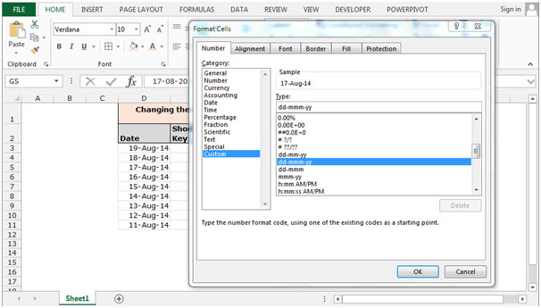
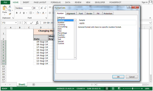
- In the Number Tab, Click on General.
- We can see the formatting in sample preview.
- The function will convert the formatting into general formatting.

To change the cell formatting by using Command Button
Follow below given steps:-
- Select the range G3:G11.
- Go to Home Tab click on General in the Number group.

- Date format will get convert in General format.
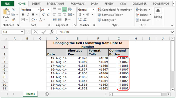
These are the ways in which we can convert the cell formatting from date to number in Microsoft Excel.
![]()
If you liked our blogs, share it with your friends on Facebook. And also you can follow us on Twitter and Facebook.
We would love to hear from you, do let us know how we can improve, complement or innovate our work and make it better for you. Write us at info@exceltip.com