
When we need to collect data from others, they may write different things from their perspective. Still, we need to make all the related stories under one. Also, it is common that while entering the data, they make mistakes because of typo errors. For example, assume in certain cells, if we ask users to enter either “YES” or “NO,” one will enter “Y,” someone will insert “YES” like this, and we may end up getting a different kind of results. So in such cases, creating a list of values as pre-determined values allows the users only to choose from the list instead of users entering their values. Therefore, in this article, we will show you how to create a list of values in Excel.
Table of contents
- Create List in Excel
- #1 – Create a Drop-Down List in Excel
- #2 – Create List of Values from Cells
- #3 – Create List through Named Manager
- Things to Remember
- Recommended Articles
You can download this Create List Excel Template here – Create List Excel Template
#1 – Create a Drop-Down List in Excel
We can create a drop-down list in Excel using the “Data Validation in excelThe data validation in excel helps control the kind of input entered by a user in the worksheet.read more” tool, so as the word itself says, data will be validated even before the user decides to enter. So, all the values that need to be entered are pre-validated by creating a drop-down list in Excel. For example, assume we need to allow the user to choose only “Agree” and “Not Agree,” so we will create a list of values in the drop-down list.
- In the Excel worksheet under the “Data” tab, we have an option called “Data Validation” from this again, choose “Data Validation.”

- As a result, this will open the “Data Validation” tool window.
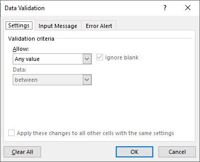
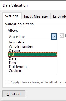
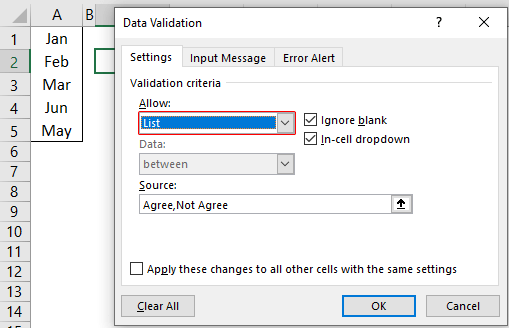
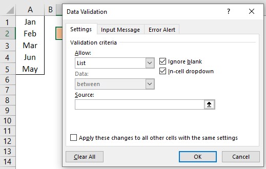
- The “Settings” tab will be shown by default, and now we need to create validation criteria. Since we are creating a list of values, choose “List” as the option from the “Allow” drop-down list.
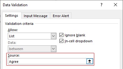
- For this “List,” we can give a list of values to be validated in the following way, i.e., by directly entering the values in the “Source” list.

- Enter the first value as “Agree.”
- Once the first value to be validated is entered, we need to enter “comma” (,) as the list separator before entering the next value. So, enter “comma” and enter the following values as “Not Agree.”
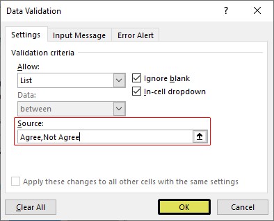
- After that, click on “Ok,” and the list of values may appear in the form of the “drop-down” list.

#2 – Create a List of Values from Cells
The above method is to get started, but imagine the scenario of creating a long list of values or your list of values changing now and then. Then, it may get difficult to return and edit the list of values manually. So, by entering values in the cell, we can easily create a list of values in Excel.
Follow the steps to create a list from cell values.
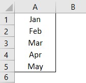
- We must first insert all the values in the cells.

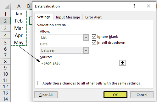
- Then, open “Data Validation” and choose the validation type as “List.”

- Next, in the “Source” box, we need to place the cursor and select the list of values from the range of cells A1 to A5.

- Click on “OK,” and we will have the list ready in cell C2.

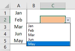
So values to this list are supplied from the range of cells A1 to A5. Any changes in these referenced cells will also impact the drop-down list.
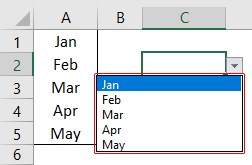
For example, in cell A4, we have a value as “Apr,” but now we will change that to “Jun” and see what happens in the drop-down list.
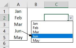
Now, look at the result of the drop-down list. Instead of “Apr,” we see “Jun” because we had given the list source as cell range, not manual entries.
#3 – Create List through Named Manager
There is another way to create a list of values, i.e., through named ranges in excelName range in Excel is a name given to a range for the future reference. To name a range, first select the range of data and then insert a table to the range, then put a name to the range from the name box on the left-hand side of the window.read more.
- We have values from A1 to A5 in the above example, naming this range “Months.”

- Now, select the cell where we need to create a list and open the drop-down list.
- Now place the cursor in the “Source” box and press the F3 key to an open list of named ranges.
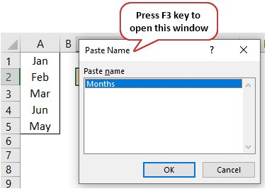
- As we can see above, we have a list of names, choose the name “Months” and click on “OK” to get the name to the “Source” box.
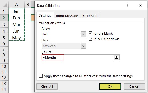
- Click on “OK,” and the drop-down list is ready.
Things to Remember
- The shortcut key to open data validation is “ALT + A + V + V.“
- We must always create a list of values in the cells so that it may impact the drop-down list if any change happens in the referenced cells.
Recommended Articles
This article has been a guide to Excel Create List. Here, we learn how to create a list of values in Excel also, create a simple drop-down method and make a list through name manager along with examples and downloadable Excel templates. You may learn more about Excel from the following articles: –
- Custom List in Excel
- Drop Down List in Excel
- Compare Two Lists in Excel
- How to Randomize List in Excel?
Create a list based on a spreadsheet
SharePoint Server Subscription Edition SharePoint Server 2019 SharePoint Server 2016 SharePoint Server 2013 SharePoint Server 2013 Enterprise SharePoint in Microsoft 365 SharePoint Server 2010 Microsoft Lists More…Less
When creating a Microsoft list, you can save time by importing an existing Excel spreadsheet. This method converts the table headings to columns in the list, and the rest of the data is imported as list items. Importing a spreadsheet is also a way to create a list without the default Title column.
Important: Creating a list from an Excel spreadsheet is not available in the GCC High and DoD environments.
Another method of moving data into SharePoint is to export a table directly from Excel. For more info, see Export an Excel table to SharePoint. For more info on SharePoint supported browsers, see Plan browser support in SharePoint Server.
Create a list based on a spreadsheet
-
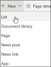
From the Lists app in Microsoft 365, select +New list or from your site’s home page, select + New > List.
-
In Microsoft Teams, from the Files tab at the top of your channel, select More > Open in SharePoint, and then select New > List.

-
-
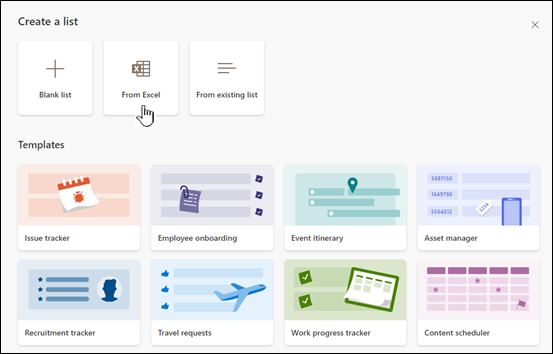
On the Create a list page, select From Excel.
-
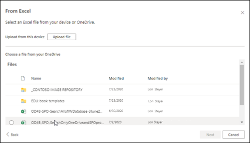
Choose Upload file to select a file on your device, or Choose a file already on this site.
If you upload from your device, the Excel file will be added to the Site Assets library of your site, which means other people will have access to the original Excel data.
Note: If the Upload file button is greyed out, you don’t have permission to create a list from a spreadsheet. For more information, see your organization’s site admin.
-
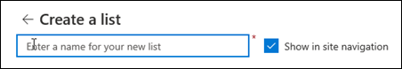
Enter the name for your list.
-
(Optional) Check Show in site navigation to display the list on your site’s Contents page.
-
Click Create.
Notes:
-
If the spreadsheet file you’re importing doesn’t have a table in it, follow the on-screen instructions to create a table in Excel, and then import the table to your list. If you get stuck creating a table, search for «Format as Table» at the top of your file in Excel.
-
You can use tables with up to 20,000 rows to create a list.
-
Create a list based on a spreadsheet in SharePoint 2016 and 2013
Note: When you’re using a site template, it is no longer possible within SharePoint to create a list from an Excel workbook. However, you can still achieve the same thing by exporting data to SharePoint from Excel, as described in Export an Excel table to SharePoint.
-
On the site where you want to add a spreadsheet based list, select Settings
, and then select Add an app. -
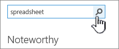
In the Find an app field, enter spreadsheet, and then select the search icon
. -
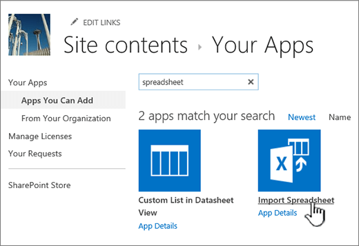
In the search results page, select Import Spreadsheet.
-
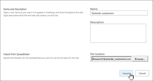
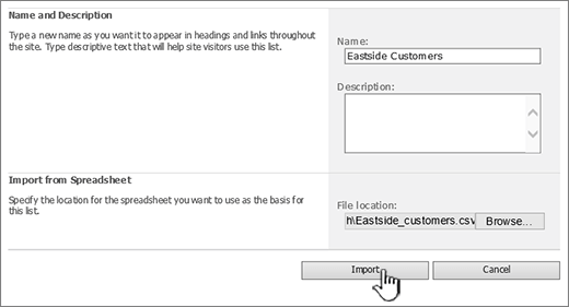
In the New app page, enter a Name for the list.
The name appears at the top of the list in most views, becomes part of the web address for the list page, and appears in site navigation to help users find the list. You can change the name of a list, but the web address will remain the same.
-
Enter an optional Description.
The description appears underneath the name in most views. You can change the description for a list at any time using list settings.
-
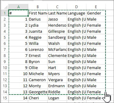
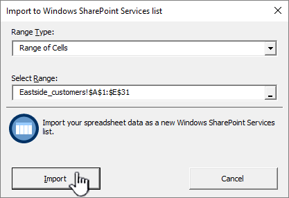
Browse to or enter the File location of the spreadsheet. When done, select Import.
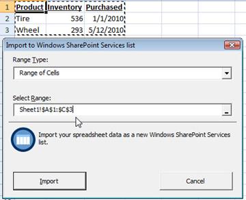
The spreadsheet opens in Excel, and the Import to Windows SharePoint Services List window appears.
-
In the Import to Windows SharePoint Services List window, select Table Range, Range of Cells, or Named Range. If you want to select a range manually, select Range of Cells, and then select Select Range. In the spreadsheet, select the upper left cell, hold down the Shift key, and select the lower right cell of the range you want.
The range appears in the Select Range field. Select Import.
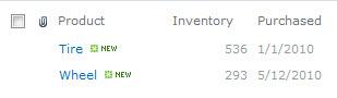
After you import a spreadsheet, check the columns of the list to make sure that the data was imported as you expected. For example, you may want to specify that a column contains currency instead of a number. To view or change list settings, open the list, select the List tab or select Settings
, and then select List Settings. -
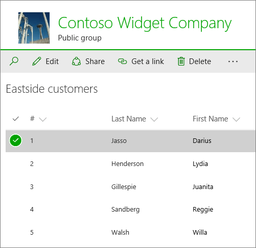
The spreadsheet data appears in a list in SharePoint.
 , and then select Add an app.
 .
.
Important: Be sure to use a 32-bit web browser, such as Microsoft Edge, to import a spreadsheet, as importing a spreadsheet relies on ActiveX filtering. Once you import the spreadsheet, then you can work with the list in any SharePoint-supported browser.
Create a list based on a spreadsheet in SharePoint 2010
-
Select Site Actions
, select View All Site Content, and then select Create .Note: A SharePoint site can be significantly modified. If you cannot locate an option, such as a command, button, or link, contact your administrator.
-
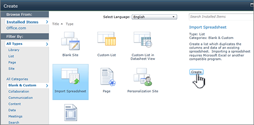
In SharePoint 2010, under All Categories, select Blanks & Custom, select Import Spreadsheet, and then select Create.
In SharePoint 2007, under Custom Lists, select Import Spreadsheet, and then select Create.
-
Enter the Name for the list. Name is required.
The name appears at the top of the list in most views, becomes part of the web address for the list page and appears in site navigation to help users find the list. You can change the name of a list at any time, but the web address will remain the same.
-
Enter the Description for the list. Description is optional.
The description appears underneath the name in most views. You can change the description for a list.
-
Browse or enter the File Location of the spreadsheet that you want to import, and then select Import.
-
In the Import to Windows SharePoint Services list dialog, select the Range Type, and in Select Range, specify the range in the spreadsheet that you want to use to create your list.
Note: Depending on your spreadsheet program, you may be able to select the range of cells that you want directly in the spreadsheet. A table range and a named range must already be defined in the spreadsheet for you to select it in the Import to Windows SharePoint Services list dialog.
-
Select Import.
 , select View All Site Content, and then select Create
  .
.
After you import a spreadsheet, check the columns of the list to make sure that the data was imported as you expected. For example, you may want to specify that a column contains currency instead of a number. To view or change list settings, open the list, select the List tab, or select Settings, and then select List Settings.
Important: Be sure to use a 32-bit web browser, such as Microsoft Edge, to import a spreadsheet, as importing a spreadsheet relies on ActiveX filtering. Once you import the spreadsheet, then you can work with the list in any SharePoint-supported browser.
The types of columns that are created for a list are based on the kinds of data that are in the columns of the spreadsheet. For example, a column in the spreadsheet that contains dates will typically be a date column in the SharePoint list.
All versions of SharePoint let you import a spreadsheet of data, though how you do it varies slightly between the versions. Examples here use Excel, but another compatible spreadsheet would work. If your spreadsheet program’s native file format isn’t supported, export your data to a comma delimited format (.CSV) and import using that file.
For more info about how to customize and add your imported list to a page or site, see Introduction to lists.
Note: Typically, the columns are set up on the SharePoint site based on the type of data that they contain. After you import a list, however, you should inspect the columns and data to make sure that everything was imported as you expected. For example, you may want to specify that a column contains currency rather than just a number. To view or change the list settings, open the list, and on the Settings menu, select List Settings.
Top of Page
Leave us a comment
Was this article helpful? If so, please let us know at the bottom of this page. If it wasn’t helpful, let us know what was confusing or missing. Please include your version of SharePoint, OS, and browser. We’ll use your feedback to double-check the facts, add info, and update this article.
Need more help?
note: please see the update on the bottom of this article for an even quicker way to convert a table
In a dark past I was an Excel instructor (among other things). I have trained countless people in the art of Excel number wizardry. I have then become a certified Excel VBA specialist, and I must say, in my years being a professional programmer, this is the skill that has set me apart from all other programmers around me. Sure, people can do Regular Expressions… So can I. Sure, people can do Object Orientation. So can I. But what programmer fancies dumb jumbling of data, and programming a language that has the word ‘basic’ in it? Right. Most programmers I knew were Linux shell companies (pun intended) that had no idea something good was hidden up the sleeve of Microsoft. But ok, sometimes I was able to show them some awesome things, and they would instantly recognize that their world view (Excell is for end-users) was a grave mistake.
What fun it was to teach people Excel, and more so, VBA! To me, it’s the tool of all tools, and it can greatly help anyone who ever works with data (ehm, anyone). So in this first part of a long, long series (I hope) I will show you, the humble ignorant user how to convert an Excel table to a list.
Why? Many times I have gone to companies and helped them with some particular problem. Usually it started out with an analyst/marketer/ceo showing me a bunch of data. The data was always presented as a table, with column headings and row headings, with the data in the middle. That seems like a nice way to present data, yes, it is in fact. The first thing I would do is then convert this table to an ugly list.
So why would you convert it to a list?
Because Excel is in love with lists. Excel craves lists, it’s like Access’ little brother, but it can speak five languages and juggle 4 balls. It’s no database tool (maximum of 65535 rows, 1M in Excel 2007)… but it can transform any list into a deep, deep analysis.
The way this analysis is done later on is with Pivot Tables. I wrote those capitals on purpose. Pivot Tables are so powerful that you can basically give it any data list and it can tell you what’s missing, what’s wrong, what’s unique, what’s the total, what’s the average, you name it. But more on that later on.
Let’s convert!
Warning: code ahead…
A table consists of three parts:
- The row headings (left)
- The column headings (top)
- The data (center)
We will loop through the data cell by cell, and create a row in a new list for each. That’s the basic idea (pun intended).
Before we start, we check some preconditions. We have to make sure that we are inside a set of data, formed into a table. All we do is just check if we have at least two rows and two columns (not the ultimate, but it works).
Sub TableToList()
If ActiveCell.CurrentRegion.Rows.Count < 2 Then
Exit Sub
End If
If ActiveCell.CurrentRegion.Columns.Count < 2 Then
Exit Sub
End If
Then we will need some variables to refer to the various sections of the table
Dim table As Range
Dim rngColHead As Range
Dim rngRowHead As Range
Dim rngData As Range
Dim rngCurrCell As Range
Next. we will need some variables for the data itself
Dim rowVal As Variant
Dim colVal As Variant
Dim val As Variant
Now, we will start pointing our variables to the data, row headings and column headings, like so
Set table = ActiveCell.CurrentRegion
Set rngColHead = table.Rows(1)
Set rngRowHead = table.Columns(1)
Set rngData = table.Offset(1, 1)
Set rngData = rngData.Resize(rngData.Rows.Count - 1, rngData.Columns.Count - 1)
Note that “currentregion” is a handy tool that expands any cell into a surrounding of non-empty cells. So this way your selected cell could be anywhere inside the table when you run the macro. The data part is a bit harder, line 4 and 5 together shift and resize the original table to form the right bottom part, where all the data resides.
ActiveWorkbook.WorkSheets.Add
Next, we create a new sheet in the workbook, to hold the list.
ActiveCell.Value = "Row#"
ActiveCell.Offset(0, 1).Value = "RowValue"
ActiveCell.Offset(0, 2).Value = "ColValue"
ActiveCell.Offset(0, 3).Value = "Data"
ActiveCell.Offset(1, 0).Select
In this sheet, we create a first row, “manually”, where we name the column headings for our list. These column headings are very important for sorting, analysis, pivot tables, export and such. The last statement instantly moves the current cell selection one row down. Notice we’re inserting a special column for Row Number. This is not always necessary, but it doesn’t hurt, and it helps you to always be able to restore the original order of the list.
Now it’s time for the actual grunt work, looping through the table
Dim n As Long
For Each rngCurrCell In rngData
colVal = rngColHead.Cells(rngCurrCell.Column - table.Column + 1)
rowVal = rngRowHead.Cells(rngCurrCell.Row - table.Row + 1)
The “for each rngCurrCell in” is a real beauty in VBA. It just runs through any selection, without worries of overflows, row and column numbers, or calculations. In the loop, we set the value of the current column and row. Note that the rngCurrCell.column and rngCurrCell.row are not relative, it’s the actual number of the column/row. So if the tables starts at C3, the first cel is having column=3 and row=3.
n = n + 1
ActiveCell.Value = n
Here, we upped counter ‘n’ and put it in the list.
ActiveCell.Offset(0, 1).Value = rowVal
ActiveCell.Offset(0, 2).Value = colVal
ActiveCell.Offset(0, 3).Value = rngCurrCell.Value
ActiveCell.Offset(1, 0).Select
We do the same trick again to put a new row in the data list on our new sheet. As you can see this part of code is repeated from the part where we created the header. A small improvement would be to create a function named ‘newRow(n, rv, cv, dv)’ to insert a new row with these values.
If, instead of actual values, you prefer to link to the original cell, you can use
ActiveCell.Offset(0, 3).Value = "=" & rngCurrCell.Worksheet.Name & "!" & rngCurrCell.Address
Finish the loop with:
Next
End Sub
Well, that’s it!
Running your code
Make sure to have a table setup in Excel, and click inside the table, it will be automatically selected.
- Press ALT+F8
- Select TableToList
- Click Run
In Office 2003 you can add a shape to your worksheet, right click, and choose assign macro.
- Choose Tools > Customize
- Choose Macros > Custom menu item -> drag to toolbar
- Right click item
- Choose Assign macro…
- Choose TableToList
Since Office 2007 this option is not available anymore, but you can still right click the ribbon and choose ‘customize quick access toolbar’. From there you can pick the Macro’s category and add the macro.
A new sheet will be created. Take a look at the list. You can try sorting, filtering, analyzing, totalling, and… pivot tables. A pivot table is a dynamically updating table which automatically totals values from a list, and presents them in… a table. Here’s how to re-create the original table from the list:”
- Choose Data > Pivot Table
- Choose Finish
- Drag ColumnValues to the ‘column fields’
- Drag RowValues to the ‘row fields’
- Drag Data into ‘Drop data items here’
Voila, the list is back. That is, if it was a list of numbers. Pivot Tables are for numeric operations, if you had text in there, it won’t show anything (anything good).
Download
Download the file here:
Table2List.xla
How to install:
- Office 2003: to install an XLA you need to go to Tools > AddIns and select the file with the browse button. Make sure the checkbox is enabled.
- Office 2007: Click on the Office Button in the left top, then Excel Options, then Add-Ins. Now select Manage… Excel Addins and click Go. Again browse and enable the addin.
You may wish to copy the file to the suggested Add-Ins folder. If you are on a network and wish to share the add-in with others, make sure to keep it on a network drive.
Once the Add-in is enabled you will see a new button that runs the macro. In Office 2007 the button is under the Add-Ins ribbon tab. You can also press ALT+F8, then type ‘Table2List.xla!TableToList’. The macro will be hidden in the XLA file, so you cannot select it.
An even quicker solution
Abu Yahya (see comments) gave me an even quicker solution. All kudos go to him for this.
First, start the pivot table wizard. Now in Excel 2007 and up you may have a hard time finding it! So, right click the quick access toolbar (it’s the bar with tiny icons on the top). Then choose Customize… and select Choose commands from: Commands not in the ribbon. Now find “pivottable and pivotchart wizard” in the list, and add it to the list on the right. You will see a tiny pivottable icon in the toolbar now.
Go on and click that icon, and then:
Step 1. Choose multiple consolidation ranges
Step 2. Choose I will create the page fields
Step 2b. Select Range of the table then Add to
Step 3. Choose New Worksheet
Step 4. Click Finish
Step 5. on the new sheet – Pivot table field list –> uncheck [ ] Row and [ ] Column
Step 6. There will be one value exactly in your pivottable. Double click it.
You will now see a new sheet with a list built up of the columns Row, Column and Value.
Step 7 (optional). Create a pivottable from this list to analyze your data.
One important note: you can have exactly 1 field that will show up in your data next to your row and column fields. That field has to be in the far left column of the data you select before consolidating. If you need more data in your final analysis you can combine fields with the “&” operator, using a formula like e.g.in cell C2: =A2 & B2.
What is Data Validation, and how does it work?
The data validation tool in Microsoft Excel allows you to limit what can be entered in your worksheet. You can, for example:
restrict entries, such as a date range or entire integers, by creating a drop down list of objects in a cell Make specific rules for what can be entered exclusively.

What Is a Drop Down List and How Do I Make One?
You can build a dropdown list of options in a cell using Data Validation. There are three simple steps to follow:
1. Make a table of contents OR a list
2. Give the List a Name
3. Make the drop-down menu
Data validation is not without flaws. It can be avoided by pasting data into the cell or using the Ribbon’s Home tab’s Clear > Clear All option.


I have a table of tools that are currently on our construction sites with how many of each tool is on each site which looks something like this:

I’m trying to create a formula that will list the tools that are on the site and skip those that aren’t with the quantity listed next to the tool. I tried creating a drop down list of the top row that will determine which column the formula looks down — seemed simple enough on paper but I’m struggling to put it into practice.
Any advice is appreciated. Thanks
![]()
asked Dec 14, 2018 at 12:12
![]()
4
If you prefer to complete your task with VBA code try:
Sub test2()

    Dim i As Long, LastCol As Long, LastRow As Long, j As Long, AddCol As Long, LastRowNew As Long
    Dim SiteName As String

    With ThisWorkbook.Worksheets("Sheet1")

        LastCol = .Cells(2, .Columns.Count).End(xlToLeft).Column
        LastRow = .Cells(.Rows.Count, "A").End(xlUp).Row

        AddCol = 3

        For i = 3 To LastCol

            .Cells(1, LastCol + AddCol).Value = .Cells(1, i).Value

            For j = 2 To LastRow
                If .Cells(j, i).Value <> 0 Then
                    LastRowNew = .Cells(.Rows.Count, (LastCol + AddCol)).End(xlUp).Row
                    .Cells(LastRowNew + 1, LastCol + AddCol).Value = .Cells(j, i).Value
                    .Cells(LastRowNew + 1, (LastCol + AddCol) - 1).Value = .Cells(j, 2).Value
                End If

            Next j

            AddCol = AddCol + 3

        Next i

    End With

End Sub
Output:

answered Dec 14, 2018 at 13:34
![]()
Error 1004Error 1004
7,8253 gold badges21 silver badges46 bronze badges
Bottom Line: Learn 4 different techniques for creating a list of numbers in Excel. These include both static and dynamic lists that change when items are added or deleted from the list.
Skill Level: Beginner
Watch the Tutorial
Download the Excel File
You can download the worksheet that I use in the video here:
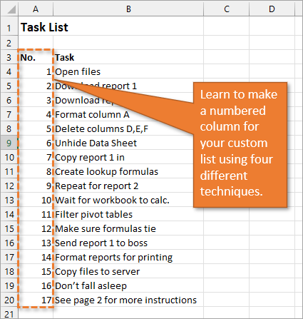
If you have a list of items in Excel and you’d like to insert a column that numbers the items, there are several ways to accomplish this. Let’s look at four of those ways.
1. Create a Static List Using Auto-Fill
The first way to number a list is really easy. Start by filling in the first two numbers of your list, select those two numbers, and then hover over the bottom right corner of your selection until your cursor turns into a plus symbol. This is the fill handle.
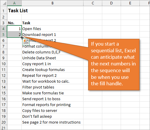
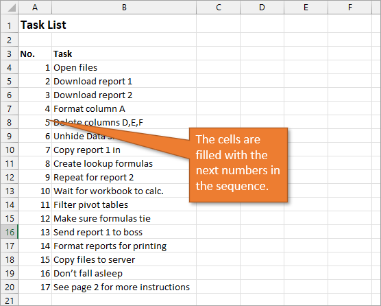
When you double-click on that fill handle (or drag it down to the end of your list), Excel will fill in the blanks with the next numbers in the sequence.
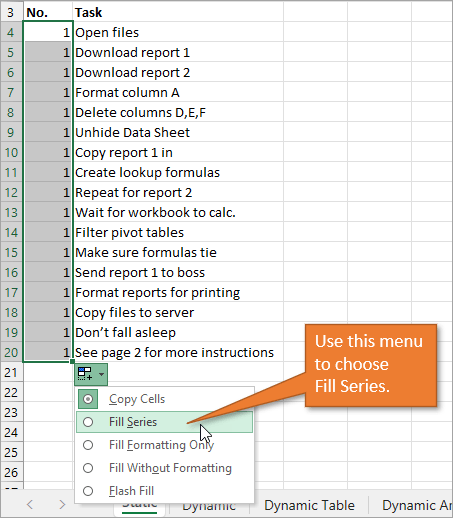
An alternate way to create this same numbered list is to type a 1 in the first cell and then double-click the fill handle. Because Excel doesn’t have a second number to identify a sequence or pattern, it will fill down the columns with 1s. But you will notice that a menu is available at the end of your column, and from that menu, you can select the option to Fill Series. This will change the 1s to a sequential list of numbers.
The numbered column we’ve created in both instances is static. This means it doesn’t change when you make additions or deletions to the corresponding list of items. For example, if I insert a new row in order to add another task, there is a break in the numbered column as well, and I would have to repeat the same steps to correct the list.
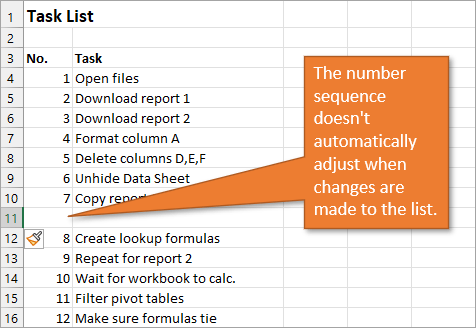
So, unless we want the numbers to always remain as they are, a better option would be to create a dynamic list.
2. Create a Dynamic List Using a Formula
We can use formulas to create a dynamic list where the numbers update when we add or delete rows from the list.
To use a formula for creating a dynamic number list, we can use the ROW function. The ROW function returns the row number of a cell. If we don’t specify a cell for ROW, it just returns the current row number of whatever is selected.
In our example, the first cell in our list doesn’t start on Row 1. It starts on Row 4. But we don’t want our list to start at 4; we want it to start at 1. To subtract the extra 3, our formula will include a minus sign and then the ROW function again, but this time pointed to the cell above our formula (which is in Row 3).
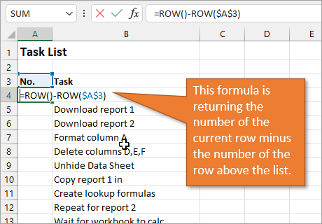
We use the absolute values (dollar signs) in our cell selection because we don’t want that number to change as we copy the formula down the list. In other words, we always want to subtract 3 from the row number to give us our list number.
When we copy down the formula, we have a numbered list that will adjust when we add or delete rows. However, when adding a row, we will have to copy the formula into the newly inserted cell.
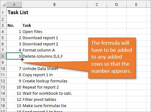
This additional step of copying the formula into new rows can be avoided if we use Excel Tables.
3. Create a Dynamic List Using a Formula in an Excel Table
If we write the same formula but we use an Excel table, the only difference we will make in the formula is that we reference the column header instead of the absolute cell value.
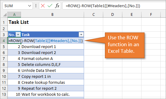
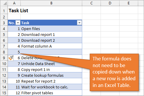
Because we are using an Excel Table, the formula automatically fills down to the other rows. When we add a row to the table, the formula will automatically populate in the new cell.
4. Create a Dynamic List Using Dynamic Array Formulas
Below, I have a table that is populated using Dynamic Array Formulas. The FILTER formula spills a range of results based on whatever name is selected in the orange cell.
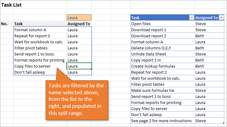
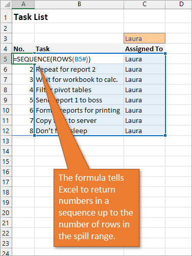
The Dynamic Array formula we will use is SEQUENCE. This will return a sequence for the number of rows we identify in the formula. To tell Excel how many rows there are, we will use the ROW function as the argument for sequence. The argument for ROW is just the spill range. The way to notate the spill range is to simply place a hashtag after the name of the first cell in the range. So our formula looks like this:
=SEQUENCE(ROWS(B5#))
Once we complete our formula and hit Enter, the list will be numbered.
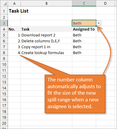
With this formula in place, if the size of the range changes when a new name is selected, the numbered column for the list will automatically adjust as well.
Bonus Tip: Formatting Your Numbered List
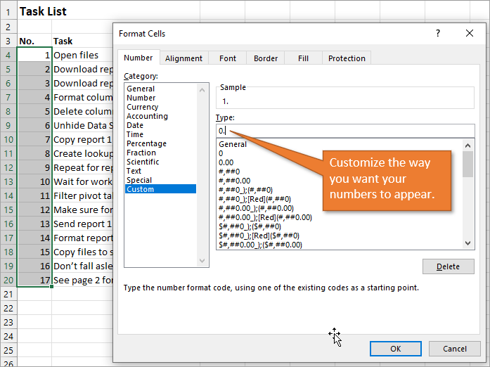
If you want to add periods or other punctuation to your numbered list:
- Select the entire list and right-click to choose Format Cells. Or use the keyboard shortcut Ctrl + 1.
- Choose the Custom option on the Number tab.
- Then in the Type field, type in the number 0 with whatever punctuation you would like to surround your number.
Here, I’ve just added a period.
When you hit OK, you will have formatted the entire selection.
Related Posts
Here are a few similar posts that may interest you.
- Excel Tables Tutorial Video – Beginners Guide for Windows & Mac
- New Excel Features: Dynamic Array Formulas & Spill Ranges
- How to Prevent Excel from Freezing or Taking A Long Time when Deleting Rows
Conclusion
I hope these four ways to create ordered lists are helpful for you. If you have questions or feedback, I would love to hear them in the comments. Have a great week!
Excel has some useful features that allow you to save time and be a lot more productive in your day-to-day work.
One such useful (and less-known) feature in the Custom Lists in Excel.
Now, before I get to how to create and use custom lists, let me first explain what’s so great about it.
Suppose you have to enter numbers the month names from Jan to Dec in a column. How would you do it? And no, doing it manually is not an option.
One of the fastest ways would be to have January in a cell, February in an adjacent cell and then use the fill handle to drag and let Excel automatically fill in the rest. Excel is smart enough to realize that you want to fill the next month in each cell in which you drag the fill handle.
Month names are quite generic and therefore it’s available by default in Excel.
But what if you have a list of department names (or employee names or product names), and you want to do the same. Instead of manually entering these or copy-paste these, you want these to appear magically when you use the fill handle (just like month names).
You can do that too…
… by using Custom Lists in Excel
In this tutorial, I will show you how to create your own custom lists in Excel and how to use these to save time.
How to Create Custom Lists in Excel
By default, Excel already has some pre-fed custom lists that you can use to save time.
For example, if you enter ‘Mon’ in one cell ‘Tue’ in an adjacent cell, you can use the fill handle to fill the rest of the days. In case you extend the selection, keep on dragging and it will repeat and give you the day’s name again.

Below are the custom lists that are already in-built in Excel. As you can see, these are mostly days and month names as these are fixed and will not change.

Now, suppose you want to create a list of departments that you often need in Excel, you can create a custom list for it. This way, the next time you need to get all the departments name in one place, you don’t need to rummage through old files. All you need to do is type the first two in the list and drag.

Below are the steps to create your own Custom List in Excel:
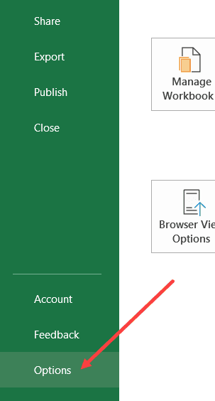
- Click the File tab

- Click on Options. This will open the ‘Excel Options‘ dialog box

- Click on the Advanced option in the left-pane

- In the General option, click on the ‘Edit Custom Lists’ button (you may have to scroll down to get to this option)

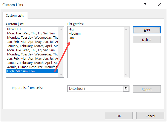
- In the Custom Lists dialog box, import the list by selecting the range of cells that have the list. Alternatively, you can also enter the name manually in the List Entries box (separated by comma or each name in a new line)

- Click on Add


As soon as you click on Add, you would notice that your list now becomes a part of the Custom Lists.

In case you have a large list that you want to add to Excel, you can also use the Import option in the dialog box.
Pro tip: You can also create a named range and use that named range to create the custom list. To do this, enter the name of the named range in the ‘Import list from cells’ field and click OK. The benefit of this is that you can change or expand the named range and it will automatically get adjusted as the custom list
Now that you have the list in Excel backend, you can use it just like you use numbers or month names with Autofill (as shown below).

While it’s great to be able to quickly get these custom lits names in Excel by doing a simple drag and drop, there is something even more awesome that you can do with custom lists (that’s what the next section is about).
Create Your Own Sorting Criteria Using Custom Lists
One great thing about custom lists is that you can use it to create your own sorting criteria. For example, suppose you have a dataset as shown below and you want to sort this based on High, Medium, and Low.

You can’t do this!
If you sort alphabetically, it would screw the alphabetical order (it will give you High, Low, and Medium and not High, Medium, and Low).
This is where Custom Lists really shine.
You can create your own list of items and then use these to sort the data. This way, you will get all the High values together at the top followed by the medium and low values.
The first step is to create a custom list (High, Medium, Low) using the steps shown in the previous section (‘How to Create Custom Lists in Excel‘).
Once you have the custom list created, you can use the below steps to sort based on it:
- Select the entire dataset (including the headers)
- Click the Data tab

- In the Sort and Filter group, click on the Sort icon. This will open the Sort dialog box

- In the Sort dialog box, make the following selections:
- Sort by Column: Priority
- Sort On: Cell Values
- Order: Custom Lists. When the dialog box opens, select the sorting criteria you want to use and then click on OK.

- Click OK


The above steps would instantly sort the data using the list you created and used as criteria while sorting (High, Medium, Low in this example).

Note that you don’t necessarily need to create the custom list first to use it in sorting. You can use the above steps and in Step 4 when the dialog box opens, you can create a list right there in that dialog box.
Some Examples Where you can Use Custom Lists
Below are some of the cases where creating and using custom lists can save you time:
- If you have a list that you need to enter manually (or copy-paste from some other source), you can create a custom list and use that instead. For example, this could be department names in your organization, or product names or regions/countries.
- If you’re a teacher, you can create a list of your student names. That way, when you are grading them the next time, you don’t need to worry about entering the student names manually or copy-pasting it from some other sheet. This also ensures that there are fewer chances of errors.
- When you need to sort data based on criteria that are not in-built in Excel. As covered in the previous section, you can use your own sorting criteria by making a custom list in Excel.
So this is all that you need to know about Creating Custom Lists in Excel.
I hope you found this useful.
You may also like the following Excel tutorials:
- How to Sort by the Last Name in Excel
- How to SORT in Excel (by Rows, Columns, Colors, Dates, & Numbers)
- How to Sort By Color in Excel
- How to Sort Worksheets in Excel
- Automatically Sort Data in Alphabetical Order using Formula
Previously I did a tutorial called «How To Extract A Dynamic List From A Data Range Based On A Criteria Without Filters In Excel». I received a question of how to modify the formula if names were added, especially at the top of the list. This tutorial addresses that question.
You can find the previous post here.
You can download the file here and follow along. When you get a preview, look for Download in the upper right hand corner.
To understand fully the process and benefits of this concept, please take a few minutes to watch the previous video from the link indicated above. In that video we used several similar formulas. The one we’ll focus on in cell «E2» of the original worksheet is:
{=IFERROR(INDEX($A$2:$A$26,SMALL(IF($B$2:$B$26=$K$1,ROW($A$2:$A$26)),
ROW(1:1))-1,1),»»)}
As you can see, it’s basically an INDEX formula wrapped in an IFERROR statement. The challenge was to make the formulas in column «E» (and similar formulas in column «H») more dynamic so if we added any entries to the main list, whether at the top, in the middle, or at the bottom, the formulas would properly extract the correct information. I created two methods to do this:
OPTION #1: OFFSET
I modified the formula in cell «E2» as follows:
Có thể bạn quan tâm
- Làm cách nào để tạo lịch 2023 trong Excel?
- Lịch Philippines 2023 với các ngày lễ có thể in Excel
- A sales call from a telemarketer is an example of which type of promotion
- What role can economies of scale play in increasing the gains from trade?
- The heat from an electric curling iron can be tested by:
{=IFERROR(INDEX(OFFSET($A$1,1,0,COUNTA($A:$A)-1,1),SMALL(IF(
OFFSET($B$1,1,0,COUNTA($A:$A)-1,1)=$K$1,ROW(OFFSET($A$1,1,0,COUNTA($A:$A)-1,1))),
ROW(1:1))-1,1),»»)}
Basically, all I did was replace the static range for the INDEX, IF, and ROW formulas with OFFSET formulas. Let’s take the array from the INDEX formula as an example. In the original formula, the array was:
$A$2:$A$26
In the new formula, we’ve modified it to be:
OFFSET($A$1,1,0,COUNTA($A:$A)-1,1)
Let’s see how this works. I’ve used the OFFSET function in many of my tutorials. If you want to see many of the uses of this function, click on OFFSET in the right column under «Excel Tutorial Topics» and you’ll see about a dozen different tutorials using the versatile function.
=OFFSET(reference,rows,cols,[height],[width])
OFFSET basically says «give me an anchor point (reference) then from that point, tell me how many rows down and how many columns over from that point do you want to go. In many formulas in which you only need to reference a single cell, that’s all you will need to use. There are two other optional arguments you may use if you want to define a range rather than a single cell, one to define how many rows high the range will be, the other how many columns wide.
So let’s break down our OFFSET formula:
Reference: $A$1 this cell is our anchor point
Rows: 1 this is telling Excel to go down one row from cell A1, which is the start of the list of names
Cols: 0 this is telling Excel not to go over any columns. We want to have our range start at cell A2
[height]: COUNTA($A:$A)-1 here we’re telling Excel that we want the range to be as many rows high as there are items in column A, minus one to account for the header of that column
[width]: 1 we only want the list of names in the INDEX array, so we want the range to be only one column wide
Looking at the formula, you’ll see that we used similar logic for the IF and ROW functions.
Take some time to get familiar with the OFFSET function and I think you’ll find it an invaluable tool!
OPTION #2: TABLE
This option is quite simple and basic. Convert the main list to a table, then reference the table name and column name in the formula instead of either a static range or, as we did with Option #1, a formula like OFFSET.
In our example, I’ve named the table «Donors». So the formula in cell «E2» now looks like this:
{=IFERROR(INDEX(Donors[Guest],SMALL(IF(Donors[Attending]=$K$1,ROW(Donors[Guest])),
ROW(1:1))-1,1),»»)}
Now, instead of the static range:
$A$2:$A$26
or the formula alternative:
OFFSET($A$1,1,0,COUNTA($A:$A)-1,1)
this (and the other ranges in the formula) can be replaced by the table reference, the example being:
Donors[Guest] («Donor» being the table name, and «Guest» being the column header)
Tables are a phenomenal tool in Excel and one that you must become familiar with. There are so many benefits to using tables. If you are not familiar or comfortable with tables in Excel, please take a moment to see this tutorial on the benefits of tables over ranges here.
What can you do next?
Share this post with others that can benefit from it!
Leave a comment or reply below let me know what you think!
Subscribe to this blog for more great tips in the future!
Check out my YouTube channel click on the YouTube icon below!
Happy Excelling!
-
03-09-2019, 08:02 PM
#1
Registered User
Trying to create a list from a table.
I need to create a list from a table of data. I have used the match function on my data input worksheet to reference a row in my table worksheet, but I’m struggling on populating a list from the table. I have very little experience with Excel, and I’m not sure how to phrase my commands. I hope someone out there can make sense of this.
Regards,
Mile299
-
03-09-2019, 08:23 PM
#2
Re: Trying to create a list from a table.
It would help if you attached a sample Excel workbook.
To do this, click on Go Advanced (below the Edit Window) while you are composing a reply, then scroll down to and click on
Manage Attachments and the Upload window will open. Click on Browse and navigate to (and double-click) the file icon that you want to attach, then click on Upload and then on Close this Window to return to the Edit window. When you have finished composing your post, click on Submit Post. Don’t try to use the Paperclip icon (Attachments button), as it doesn’t work on this forum.
Hope this helps.
Pete
-
03-09-2019, 11:47 PM
#3
Registered User
Re: Trying to create a list from a table.
Sorry, I should have guessed that. Please find the file attached. The list1! table is what I am trying to use to populate a drop-down list in the data input page.
I want to be able to use excel to manage different pipe wall thicknesses for the work that I’m doing, This about version four of this project, and I think maybe
it is better to just ask for advice.Thank you for your time,
Mile299
-
03-10-2019, 05:29 PM
#4
Re: Trying to create a list from a table.
Named ranges:
Data val for pipe sizes: =SizeList
dv for schedules: =schedules
lookup O.D.: =VLOOKUP(D3,Table1[[#All],[Size]:[O.D.]],2,FALSE)
wall thickness intersects size and sched: =INDEX(Table1,MATCH(NPS,SizeList,0),MATCH(Sched,schedules,0)+2)

