Excel counting rows in a range - Word и Excel - помощь в работе с программами

Select the cell where you want the result to appear.
On the Formulas tab, click More Functions, point to Statistical, and then click one of the following functions:
- COUNTA: To count cells that are not empty
- COUNT: To count cells that contain numbers.
- COUNTBLANK: To count cells that are blank.
- COUNTIF: To count cells that meets a specified criteria.
  
  Tip: To enter more than one criterion, use the COUNTIFS function instead.
Select the range of cells that you want, and then press RETURN.

Select the cell where you want the result to appear.
On the Formulas tab, click Insert, point to Statistical, and then click one of the following functions:
- COUNTA: To count cells that are not empty
- COUNT: To count cells that contain numbers.
- COUNTBLANK: To count cells that are blank.
- COUNTIF: To count cells that meets a specified criteria.
  
  Tip: To enter more than one criterion, use the COUNTIFS function instead.
Select the range of cells that you want, and then press RETURN.

This tutorial shows how to count the total number of rows from a selected range through the use of an Excel formula or VBA

Example: Count number of rows in a range

METHOD 1. Count number of rows in a range

EXCEL

This formula uses the Excel ROWS function to return the number of rows in the selected range. In this example we have selected range (E5:E15) inside the ROWS function, which returns a total of 11 rows.

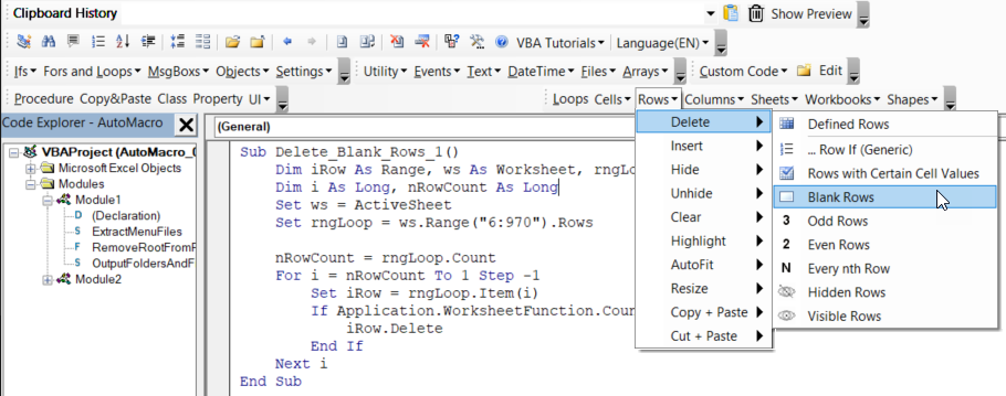
METHOD 1. Count number of rows in a range using VBA

VBA

Sub Count_number_of_rows_in_range()

‘declare a variable
Dim ws As Worksheet

Set ws = Worksheets(«Analysis»)

‘count the total number of rows in a specific range
ws.Range(«B5») = ws.Range(«E5:E15»).Rows.Count

End Sub

ADJUSTABLE PARAMETERS
Output Range: Select the output range by changing the cell reference («B5») in the VBA code.
Range: Select the range from which you want to count the number of rows by changing the range reference («E5:E15») in the VBA code.
Worksheet Selection: Select the worksheet in which you want to count the number of rows from a selected range by changing the Analysis worksheet name in the VBA code. You can also change the name of this object variable, by changing the name ‘ws’ in the VBA code.

Explanation about the formula used to count number of rows in a range

EXPLANATION

This tutorial shows how to count the total number of rows from a selected range through the use of an Excel formula or VBA.

Both the Excel formula and VBA approach make use of the ROWS function to count the number of rows in a selected range.

Using the VBA method you will also need to combine the Rows function with the Count function to return the total number of rows in a selected range.

FORMULA
=ROWS(array)

ARGUMENTS
array: An array or reference to a range of cells.

Related Topic	Description	Related Topic and Description
Count number of columns in a range	How to count the total number of columns in a range using Excel and VBA methods
Count number of cells in a range	How to count the total number of cells in a range using Excel and VBA methods
Count number of characters in a cell	How to count the total number of characters, including spaces, in a cell using Excel and VBA methods
Count number of characters in a cell excluding spaces	How to count the total number of characters in a cell, excluding spaces, using Excel and VBA methods
Count number of characters in a range	How to ccount the total number of characters in a range, including spaces, using Excel and VBA methods

Related Functions	Description	Related Functions and Description
ROWS Function	The Excel ROWS function returns the number of rows in a specified array

Источник

How to Count the Number of Rows in Excel?

Here are the different ways of counting rows in Excel using the formula, rows with data, empty rows, rows with numerical values, rows with text values, and many other things related to counting the number of rows in Excel.

You can download this Count Rows Excel Template here – Count Rows Excel Template

How to Count the Number of Rows in Excel?
- #1 – Excel Count Rows which has only the Data
- #2 – Count all the rows that have the data
- #3 – Count the rows that only have the numbers
- #4 – Count Rows, which only has the Blanks
- #5 – Count rows that only have text values
- #6 – Count all of the rows in the range
- Things to Remember
- Recommended Articles

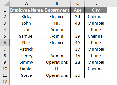
#1 – Excel Count Rows which has only the Data

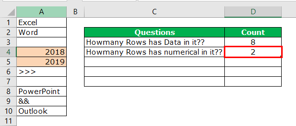
Firstly, we will see how to count the number of rows in Excel with the data. There could be empty rows between the data, but we often need to ignore them and find exactly how many rows contain the data in it.

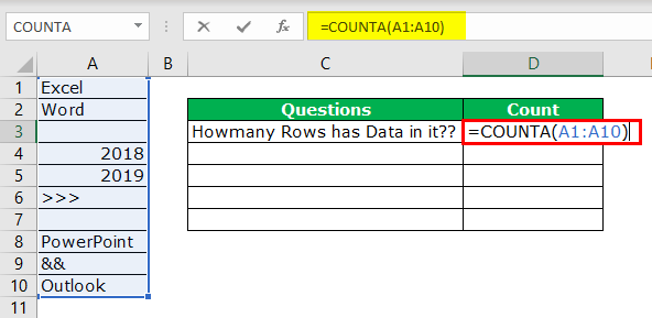
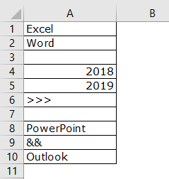
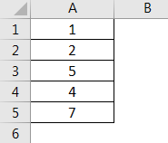
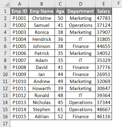
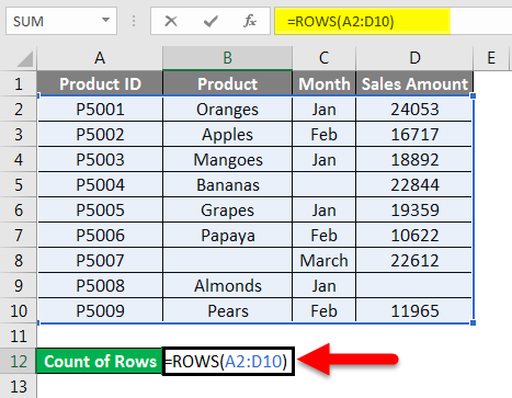
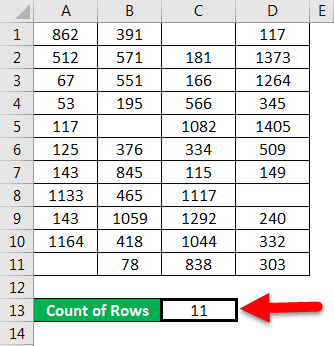
We can count the number of rows with data by selecting the range of cells in Excel. For example, take a look at the below data.

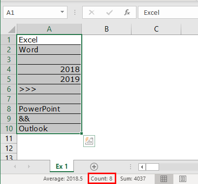
We have a total of 10 rows (border inserted area). In this 10 row, we want to count exactly how many cells have data. Since this is a small list of rows, we can easily calculate the number of rows. But when it comes to the huge database, it is impossible to count manually. So, this article will help you with this.
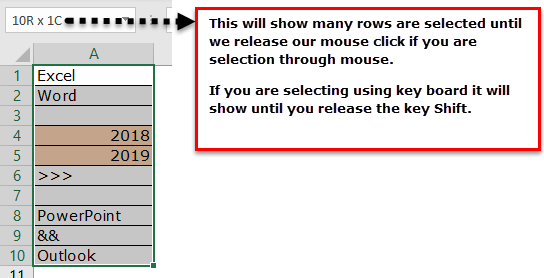
Firstly, we must select all the rows in Excel.
It is not telling us how many rows contain the data here. Instead, look at the Excel screen’s right-hand side bottom, i.e., a status bar.

Take a look at the red circled area. It says COUNT as 8, which means that out of 10 selected rows, 8 have data.
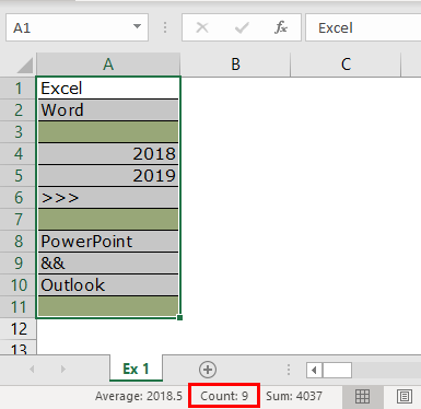
Now, we will select one more row in the range and see what the count will be.
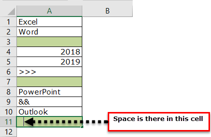
We have selected 11 rows, but the count says 9, whereas we have data only in 8 rows. When we closely examine the cells, the 11th row contains a space.

Even though there is no value in the cell and it has only space Excel will be treated as the cell which contains the data.

#2 – Count all the rows that have the data

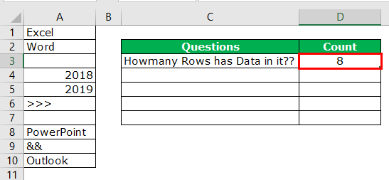
We know how to check how many rows contain the data quickly. But that is not the dynamic way of counting rows that have data. Instead, we need to apply the COUNTA function to count how many rows contain the data.

We will apply the COUNTA function in the D3 cell.

So, the total number of rows containing the data is 8 rows. Even this formula treats space as data.

#3 – Count the rows that only have the numbers

Here we want to count how many rows contain only numerical values.

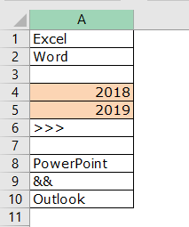
We can easily say 2 rows contain numerical values. Let us examine this by using a formula. We have a built-in formula called COUNT which counts only numerical values in the supplied range.

We will apply the COUNT function in cell B1 and select the range as A1 to A10.

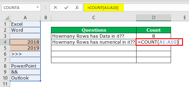
The COUNT function also says 2 as a result. So, out of 10 rows, only rows contain numerical values.

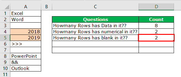
#4 – Count Rows, which only has the Blanks

We can find only blank rows by using the COUNTBLANK function in Excel.

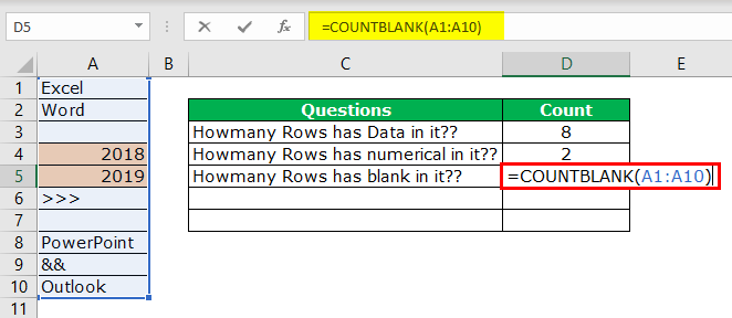
We have 2 blank rows in the selected range, which are revealed by the count blank function.

#5 – Count rows that only have text values

Remember, we do not have any straight in the COUNTTEXT function. Unlike in previous cases, we need to think differently here. We can use the COUNTIF functionThe COUNTIF function in Excel counts the number of cells within a range based on pre-defined criteria. It is used to count cells that include dates, numbers, or text. For example, COUNTIF(A1:A10,”Trump”) will count the number of cells within the range A1:A10 that contain the text “Trump”
read more with a wildcard character asterisk (*).

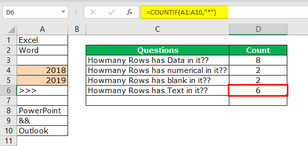
Here all the magic is done by the wildcard character asterisk (*). It matches any of the alphabets in the row and returns the result as a text value row. Even if the row contains numerical and text values, it will be treated as text value only.

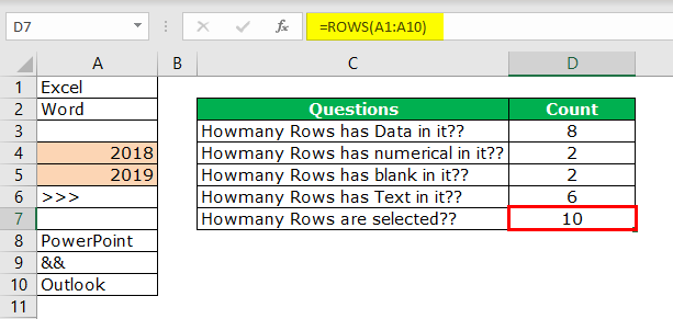
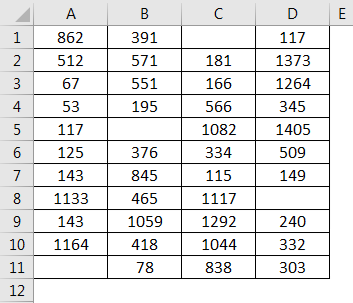
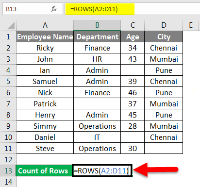
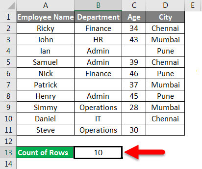
#6 – Count all of the rows in the range

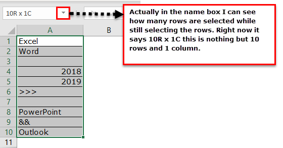
Now comes the important part. How do we count how many rows we have selected? One uses the Name Box in excel, which is limited while still choosing the rows. But how do we measure then?

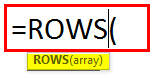
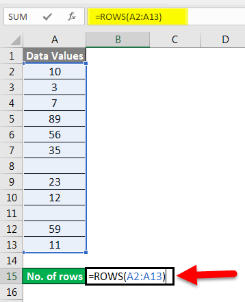
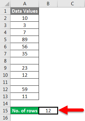
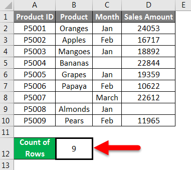
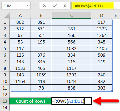
We have a built-in ROWS formula, which returns how many rows are selected.

Things to Remember

Even space is treated as a value in the cell.
If the cell contains numerical and text values, it will be treated as a text value.
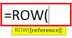
ROW may return the current row we are in, but ROWS will return how many are in the supplied range even though there is no data in the rows.

Свойство Range.Rows (Excel)

Возвращает объект Range , представляющий строки в указанном диапазоне.

Синтаксис

expression. Строк

выражение: переменная, представляющая объект Range.

Замечания

Чтобы вернуть одну строку, используйте свойство Item или аналогично включите индекс в круглые скобки. Например, и Selection.Rows(1) Selection.Rows.Item(1) возвращают первую строку выделенного фрагмента.

При применении к объекту Range , который является множественным выделением, это свойство возвращает строки только из первой области диапазона. Например, если объект someRange Range имеет две области — A1:B2 и C3:D4, someRange.Rows.Count возвращает значение 2, а не 4. Чтобы использовать это свойство в диапазоне, который может содержать несколько выделенных элементов, проверьте Areas.Count , чтобы определить, является ли диапазон множественным выбором. Если это так, выполните цикл по каждой области диапазона, как показано в третьем примере.

Возвращаемый диапазон может находиться за пределами указанного диапазона. Например, Range(«A1:B2»).Rows(5) возвращает ячейки A5:B5. Дополнительные сведения см. в разделе Свойство Item .

Использование свойства Rows без квалификатора объекта эквивалентно использованию ActiveSheet.Rows. Дополнительные сведения см. в свойстве Worksheet.Rows .

Пример

В этом примере удаляется диапазон B5:Z5 на листе 1 активной книги.

В этом примере строки в текущем регионе удаляются на листе одной из активных книг, где значение ячейки в строке совпадает со значением ячейки в предыдущей строке.

В этом примере отображается количество строк в выделенном фрагменте на листе Sheet1. Если выбрано несколько областей, в примере выполняется цикл по каждой области.

Поддержка и обратная связь

Есть вопросы или отзывы, касающиеся Office VBA или этой статьи? Руководство по другим способам получения поддержки и отправки отзывов см. в статье Поддержка Office VBA и обратная связь.

Источник

Count Rows in Excel

How to Count the Number of Rows in Excel?

Here are the different ways of counting rows in Excel using the formula, rows with data, empty rows, rows with numerical values, rows with text values, and many other things related to counting the number of rows in Excel.

#1 – Excel Count Rows which has only the Data

We can count the number of rows with data by selecting the range of cells in Excel. For example, take a look at the below data.

We have a total of 10 rows (border inserted area). In this 10 row, we want to count exactly how many cells have data. Since this is a small list of rows, we can easily calculate the number of rows. But when it comes to the huge database, it is impossible to count manually. So, this article will help you with this.

Firstly, we must select all the rows in Excel.

It is not telling us how many rows contain the data here. Instead, look at the Excel screen’s right-hand side bottom, i.e., a status bar.

Take a look at the red circled area. It says COUNT as 8, which means that out of 10 selected rows, 8 have data.

Now, we will select one more row in the range and see what the count will be.

We have selected 11 rows, but the count says 9, whereas we have data only in 8 rows. When we closely examine the cells, the 11th row contains a space.

Even though there is no value in the cell and it has only space Excel will be treated as the cell which contains the data.

#2 – Count all the rows that have the data

We will apply the COUNTA function in the D3 cell.

So, the total number of rows containing the data is 8 rows. Even this formula treats space as data.

#3 – Count the rows that only have the numbers

Here we want to count how many rows contain only numerical values.

We can easily say 2 rows contain numerical values. Let us examine this by using a formula. We have a built-in formula called COUNT which counts only numerical values in the supplied range.

We will apply the COUNT function in cell B1 and select the range as A1 to A10.

The COUNT function also says 2 as a result. So, out of 10 rows, only rows contain numerical values.

#4 – Count Rows, which only has the Blanks

We can find only blank rows by using the COUNTBLANK function in Excel.

We have 2 blank rows in the selected range, which are revealed by the count blank function.

#5 – Count rows that only have text values

#6 – Count all of the rows in the range

Now comes the important part. How do we count how many rows we have selected? One uses the Name Box in excel, which is limited while still choosing the rows. But how do we measure then?

We have a built-in ROWS formula, which returns how many rows are selected.

Things to Remember

Even space is treated as a value in the cell.
If the cell contains numerical and text values, it will be treated as a text value.
ROW may return the current row we are in, but ROWS will return how many are in the supplied range even though there is no data in the rows.

VBA – Count the rows in a Selection

In this Article

If you ever need to count the number of rows that were selected, use Selection.Rows.Count

Count Rows in a Selection

If you ever need to count the number of Columns that were selected, use Selection.Columns.Count

Count Columns in a Selection

VBA Coding Made Easy

Stop searching for VBA code online. Learn more about AutoMacro – A VBA Code Builder that allows beginners to code procedures from scratch with minimal coding knowledge and with many time-saving features for all users!

VBA Code Examples Add-in

Easily access all of the code examples found on our site.

Simply navigate to the menu, click, and the code will be inserted directly into your module. .xlam add-in.

(No installation required!)

VBA Code Generator

AutoMacro: VBA Add-in with Hundreds of Ready-To-Use VBA Code Examples & much more!

What is AutoMacro?

AutoMacro is an add-in for VBA that installs directly into the Visual Basic Editor. It comes loaded with code generators, an extensive code library, the ability to create your own code library, and many other time-saving tools and utilities that add much needed functionality to the outdated VBA Editor.

Источник

Ways to count values in a worksheet

Counting is an integral part of data analysis, whether you are tallying the head count of a department in your organization or the number of units that were sold quarter-by-quarter. Excel provides multiple techniques that you can use to count cells, rows, or columns of data. To help you make the best choice, this article provides a comprehensive summary of methods, a downloadable workbook with interactive examples, and links to related topics for further understanding.

Note: Counting should not be confused with summing. For more information about summing values in cells, columns, or rows, see Summing up ways to add and count Excel data.

Download our examples

You can download an example workbook that gives examples to supplement the information in this article. Most sections in this article will refer to the appropriate worksheet within the example workbook that provides examples and more information.

Simple counting

You can count the number of values in a range or table by using a simple formula, clicking a button, or by using a worksheet function.

Excel can also display the count of the number of selected cells on the Excel status bar. See the video demo that follows for a quick look at using the status bar. Also, see the section Displaying calculations and counts on the status bar for more information. You can refer to the values shown on the status bar when you want a quick glance at your data and don’t have time to enter formulas.

Video: Count cells by using the Excel status bar

Watch the following video to learn how to view count on the status bar.

Use AutoSum

Use AutoSum by selecting a range of cells that contains at least one numeric value. Then on the Formulas tab, click AutoSum > Count Numbers.

Excel returns the count of the numeric values in the range in a cell adjacent to the range you selected. Generally, this result is displayed in a cell to the right for a horizontal range or in a cell below for a vertical range.

Add a Subtotal row

You can add a subtotal row to your Excel data. Click anywhere inside your data, and then click Data > Subtotal.

Note: The Subtotal option will only work on normal Excel data, and not Excel tables, PivotTables, or PivotCharts.

Also, refer to the following articles:

Count cells in a list or Excel table column by using the SUBTOTAL function

Use the SUBTOTAL function to count the number of values in an Excel table or range of cells. If the table or range contains hidden cells, you can use SUBTOTAL to include or exclude those hidden cells, and this is the biggest difference between SUM and SUBTOTAL functions.

The SUBTOTAL syntax goes like this:

To include hidden values in your range, you should set the function_num argument to 2.

To exclude hidden values in your range, set the function_num argument to 102.

Counting based on one or more conditions

You can count the number of cells in a range that meet conditions (also known as criteria) that you specify by using a number of worksheet functions.

Video: Use the COUNT, COUNTIF, and COUNTA functions

Watch the following video to see how to use the COUNT function and how to use the COUNTIF and COUNTA functions to count only the cells that meet conditions you specify.

Count cells in a range by using the COUNT function

Use the COUNT function in a formula to count the number of numeric values in a range.

In the above example, A2, A3, and A6 are the only cells that contains numeric values in the range, hence the output is 3.

Note: A7 is a time value, but it contains text ( a.m.), hence COUNT does not consider it a numerical value. If you were to remove a.m. from the cell, COUNT will consider A7 as a numerical value, and change the output to 4.

Count cells in a range based on a single condition by using the COUNTIF function

Use the COUNTIF function function to count how many times a particular value appears in a range of cells.

Count cells in a column based on single or multiple conditions by using the DCOUNT function

DCOUNT function counts the cells that contain numbers in a field (column) of records in a list or database that match conditions that you specify.

In the following example, you want to find the count of the months including or later than March 2016 that had more than 400 units sold. The first table in the worksheet, from A1 to B7, contains the sales data.

DCOUNT uses conditions to determine where the values should be returned from. Conditions are typically entered in cells in the worksheet itself, and you then refer to these cells in the criteria argument. In this example, cells A10 and B10 contain two conditions—one that specifies that the return value must be greater than 400, and the other that specifies that the ending month should be equal to or greater than March 31st, 2016.

You should use the following syntax:

DCOUNT checks the data in the range A1 through B7, applies the conditions specified in A10 and B10, and returns 2, the total number of rows that satisfy both conditions (rows 5 and 7).

Count cells in a range based on multiple conditions by using the COUNTIFS function

The COUNTIFS function is similar to the COUNTIF function with one important exception: COUNTIFS lets you apply criteria to cells across multiple ranges and counts the number of times all criteria are met. You can use up to 127 range/criteria pairs with COUNTIFS.

The syntax for COUNTIFS is:

COUNTIFS(criteria_range1, criteria1, [criteria_range2, criteria2],…)

See the following example:

Count based on criteria by using the COUNT and IF functions together

Let’s say you need to determine how many salespeople sold a particular item in a certain region or you want to know how many sales over a certain value were made by a particular salesperson. You can use the IF and COUNT functions together; that is, you first use the IF function to test a condition and then, only if the result of the IF function is True, you use the COUNT function to count cells.

The formulas in this example must be entered as array formulas. If you have opened this workbook in Excel for Windows or Excel 2016 for Mac and want to change the formula or create a similar formula, press F2, and then press Ctrl+Shift+Enter to make the formula return the results you expect. In earlier versions of Excel for Mac, use +Shift+Enter.

For the example formulas to work, the second argument for the IF function must be a number.

Count how often multiple text or number values occur by using the SUM and IF functions together

In the examples that follow, we use the IF and SUM functions together. The IF function first tests the values in some cells and then, if the result of the test is True, SUM totals those values that pass the test.

The above function says if C2:C7 contains the values Buchanan and Dodsworth, then the SUM function should display the sum of records where the condition is met. The formula finds three records for Buchanan and one for Dodsworth in the given range, and displays 4.

The above function says if D2:D7 contains values lesser than $9000 or greater than $19,000, then SUM should display the sum of all those records where the condition is met. The formula finds two records D3 and D5 with values lesser than $9000, and then D4 and D6 with values greater than $19,000, and displays 4.

The above function says if D2:D7 has invoices for Buchanan for less than $9000, then SUM should display the sum of records where the condition is met. The formula finds that C6 meets the condition, and displays 1.

Important: The formulas in this example must be entered as array formulas. That means you press F2 and then press Ctrl+Shift+Enter. In earlier versions of Excel for Mac use +Shift+Enter.

See the following Knowledge Base articles for additional tips:

Count cells in a column or row in a PivotTable

A PivotTable summarizes your data and helps you analyze and drill down into your data by letting you choose the categories on which you want to view your data.

You can quickly create a PivotTable by selecting a cell in a range of data or Excel table and then, on the Insert tab, in the Tables group, clicking PivotTable.

Let’s look at a sample scenario of a Sales spreadsheet, where you can count how many sales values are there for Golf and Tennis for specific quarters.

Note: For an interactive experience, you can run these steps on the sample data provided in the PivotTable sheet in the downloadable workbook.

Enter the following data in an Excel spreadsheet.

Click Insert > PivotTable.

In the Create PivotTable dialog box, click Select a table or range, then click New Worksheet, and then click OK.

An empty PivotTable is created in a new sheet.

In the PivotTable Fields pane, do the following:

Drag Sport to the Rows area.

Drag Quarter to the Columns area.

Drag Sales to the Values area.

The field name displays as SumofSales2 in both the PivotTable and the Values area.

At this point, the PivotTable Fields pane looks like this:

In the Values area, click the dropdown next to SumofSales2 and select Value Field Settings.

In the Value Field Settings dialog box, do the following:

In the Summarize value field by section, select Count.

In the Custom Name field, modify the name to Count.

The PivotTable displays the count of records for Golf and Tennis in Quarter 3 and Quarter 4, along with the sales figures.

Counting when your data contains blank values

You can count cells that either contain data or are blank by using worksheet functions.

Count nonblank cells in a range by using the COUNTA function

Use the COUNTA function function to count only cells in a range that contain values.

When you count cells, sometimes you want to ignore any blank cells because only cells with values are meaningful to you. For example, you want to count the total number of salespeople who made a sale (column D).

COUNTA ignores the blank values in D3, D4, D8, and D11, and counts only the cells containing values in column D. The function finds six cells in column D containing values and displays 6 as the output.

Count nonblank cells in a list with specific conditions by using the DCOUNTA function

Use the DCOUNTA function to count nonblank cells in a column of records in a list or database that match conditions that you specify.

The following example uses the DCOUNTA function to count the number of records in the database that is contained in the range A1:B7 that meet the conditions specified in the criteria range A9:B10. Those conditions are that the Product ID value must be greater than or equal to 2000 and the Ratings value must be greater than or equal to 50.

DCOUNTA finds two rows that meet the conditions- rows 2 and 4, and displays the value 2 as the output.

Count blank cells in a contiguous range by using the COUNTBLANK function

Use the COUNTBLANK function function to return the number of blank cells in a contiguous range (cells are contiguous if they are all connected in an unbroken sequence). If a cell contains a formula that returns empty text («»), that cell is counted.

When you count cells, there may be times when you want to include blank cells because they are meaningful to you. In the following example of a grocery sales spreadsheet. suppose you want to find out how many cells don’t have the sales figures mentioned.

Note: The COUNTBLANK worksheet function provides the most convenient method for determining the number of blank cells in a range, but it doesn’t work very well when the cells of interest are in a closed workbook or when they do not form a contiguous range. The Knowledge Base article XL: When to Use SUM(IF()) instead of CountBlank() shows you how to use a SUM(IF()) array formula in those cases.

Count blank cells in a non-contiguous range by using a combination of SUM and IF functions

Use a combination of the SUM function and the IF function. In general, you do this by using the IF function in an array formula to determine whether each referenced cell contains a value, and then summing the number of FALSE values returned by the formula.

See a few examples of SUM and IF function combinations in an earlier section Count how often multiple text or number values occur by using the SUM and IF functions together in this topic.

Counting unique occurrences of values

You can count unique values in a range by using a PivotTable, COUNTIF function, SUM and IF functions together, or the Advanced Filter dialog box.

Count the number of unique values in a list column by using Advanced Filter

Use the Advanced Filter dialog box to find the unique values in a column of data. You can either filter the values in place or you can extract and paste them to a new location. Then you can use the ROWS function to count the number of items in the new range.

To use Advanced Filter, click the Data tab, and in the Sort & Filter group, click Advanced.

The following figure shows how you use the Advanced Filter to copy only the unique records to a new location on the worksheet.

In the following figure, column E contains the values that were copied from the range in column D.

If you filter your data in place, values are not deleted from your worksheet — one or more rows might be hidden. Click Clear in the Sort & Filter group on the Data tab to display those values again.

If you only want to see the number of unique values at a quick glance, select the data after you have used the Advanced Filter (either the filtered or the copied data) and then look at the status bar. The Count value on the status bar should equal the number of unique values.

Count the number of unique values in a range that meet one or more conditions by using IF, SUM, FREQUENCY, MATCH, and LEN functions

Use various combinations of the IF, SUM, FREQUENCY, MATCH, and LEN functions.

For more information and examples, see the section «Count the number of unique values by using functions» in the article Count unique values among duplicates.

Special cases (count all cells, count words)

You can count the number of cells or the number of words in a range by using various combinations of worksheet functions.

Count the total number of cells in a range by using ROWS and COLUMNS functions

Suppose you want to determine the size of a large worksheet to decide whether to use manual or automatic calculation in your workbook. To count all the cells in a range, use a formula that multiplies the return values using the ROWS and COLUMNS functions. See the following image for an example:

Count words in a range by using a combination of SUM, IF, LEN, TRIM, and SUBSTITUTE functions

You can use a combination of the SUM, IF, LEN, TRIM, and SUBSTITUTE functions in an array formula. The following example shows the result of using a nested formula to find the number of words in a range of 7 cells (3 of which are empty). Some of the cells contain leading or trailing spaces — the TRIM and SUBSTITUTE functions remove these extra spaces before any counting occurs. See the following example:

Now, for the above formula to work correctly, you have to make this an array formula, otherwise the formula returns the #VALUE! error. To do that, click on the cell that has the formula, and then in the Formula bar, press Ctrl + Shift + Enter. Excel adds a curly bracket at the beginning and the end of the formula, thus making it an array formula.

For more information on array formulas, see Overview of formulas in Excel and Create an array formula.

Displaying calculations and counts on the status bar

When one or more cells are selected, information about the data in those cells is displayed on the Excel status bar. For example, if four cells on your worksheet are selected, and they contain the values 2, 3, a text string (such as «cloud»), and 4, all of the following values can be displayed on the status bar at the same time: Average, Count, Numerical Count, Min, Max, and Sum. Right-click the status bar to show or hide any or all of these values. These values are shown in the illustration that follows.

Need more help?

You can always ask an expert in the Excel Tech Community or get support in the Answers community.

Источник

Excel Row Count (Table of Contents)

Introduction to Row Count in Excel
How to Count the Rows in Excel?

Introduction to Row Count in Excel

Excel provides many built-in functions through which we can do multiple calculations. We can also count the rows and columns in Excel. Here in this article, we will discuss the Row Count in Excel. If we want to measure the rows which contain data, select all the cells of the first column by clicking on the column header. It will display the row count on the status bar in the lower right corner.

Let’s take some values in the Excel sheet.

Select the entire column which contains data. Now click on the column label for counting the rows; it will show you the row count. Refer to the below screenshot:

There are two types of functions for counting the rows.

ROW()
ROWS()

The ROW() function gives you the row number of a particular cell.

The ROWS() function gives you the count of rows in a range.

How to Count the Rows in Excel?

Let’s take some examples to understand the usage of ROWS functions.

You can download this Row Count Excel Template here – Row Count Excel Template

Example #1

We have given the below employee data.

For counting the rows here, we will use the below function here:

=ROWS(range)

Where range = a range of cells containing data.

Now we will apply the above function like the below screenshot:

Which returns the number of rows containing the data in the supplied range.

The final result is given below:

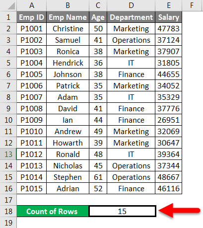
Example #2

We have given below some student marks subject-wise.

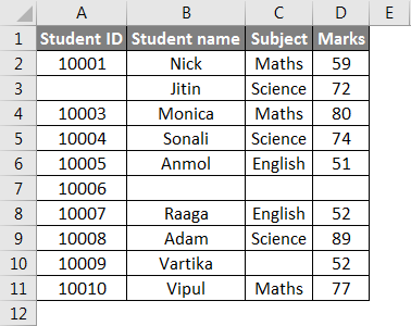
As we can see in the above dataset, certain information is absent.

As per the screenshot below, we will apply the ROWS function for counting the rows containing data.

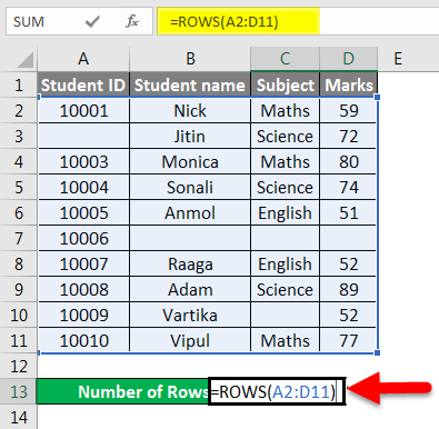
The final result is given below:

Example #3

We have given the below data values.

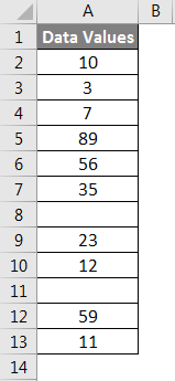
We will pass the range of data values within the function for counting the number of rows.

Apply the function like the below screenshot:

Press ENTER key here, and it will return the count of rows.

The final result is shown below:

Explanation:

When we pass the range of cells, it gives you the count of cells you selected.

Example #4

We have given below product details:

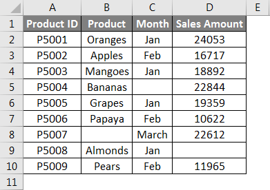
Now we will pass the range of the given dataset within the function like the below screenshot:

Press ENTER key, which will give you the count of rows containing data in the passing range.

The final result is given below:

Example #5

We have given some raw data.

Some cell values are missing here, so now, for counting the rows, we will apply the function shown in the below screenshot:

Hit the Enter key, and it will return the count of rows having data.

The final result is given below:

Example #6

We have given a company employee data where some details are missing:

Now apply the ROWS function to count the row containing data of employees:

Hit the Enter key to get the final rows

Things to Remember About Row Count in Excel

When you click on the column heading for counting the rows, it will give you the count which contains data.
If you pass a range of cells, it will return the number of cells that you have selected.
The status bar won’t show you anything if the column contains the data only in one cell. That is, the status bar stays blank.
If the data are given in the table form, then for counting the rows, you can pass the table range within the ROWS function.
You can also do the setting of the message in the status bar. Do right-click on the status bar and click the item you want to see or remove.

Recommended Articles

This article has been a guide to Row Count in Excel. Here we discussed How to Count the Rows, practical examples, and a downloadable Excel template. You can also go through our other suggested articles–

COUNTA Function in Excel
Count Function in Excel
ROWS Function in Excel
Add Rows in Excel Shortcut

Источник

Date yes Add (Subtract) Days to a Date Concatenate Dates Convert Date to Number Convert Date to Text Month Name to Number Create Date Range from Dates Day Number of Year Month Name from Date First Day of Month Add (Subtract) Weeks to a Date If Functions with Dates Max Date Number of Days Between Dates Number of Days in a Month Number of Weeks Between Dates Number of Years Between Dates Split Date & Time into Separate Cells Countdown Remaining Days Insert Dates Random Date Generator Using Dynamic Ranges — Year to Date Values Add (Subtract) Years to a Date Date Formula Examples Extract Day from Date Get Day Name from Date Count Days Left in Month / Year Count Workdays Left in Month / Year Get Last Day of Month Last Business Day of Month / Year Number of Work / Business Days in Month Weekday Abbreviations Auto Populate Dates Number of Months Between Dates Quarter from a Date Years of Service Change Date Format Compare Dates Time yes Add (Subtract) Hours to Time Add (Subtract) Minutes to Time Add (Subtract) Seconds to Time Add Up time (Total Time) Time Differences Change Time Format Convert Minutes to Hours Convert Time to Decimal Convert Time to Hours Convert Time to Minutes Convert Time to Seconds Military Time Round Time to Nearest 15 Minutes Overtime Calculator Number of Hours Between Times Convert Seconds to Minutes, Hours, or Time Count Hours Worked Time Differences Time Format — Show Minutes Seconds Text yes Add Commas to Cells Get First Word from Text Capitalize First Letter Clean & Format Phone #s Remove Extra Trailing / Leading Spaces Add Spaces to Cell Assign Number Value to Text Combine Cells with Comma Combine First and Last Names Convert Text String to Date Convert Text to Number Extract Text From Cell Get Last Word Remove Unwated Characters Extract Text Before or After Character How to Split Text String by Space, Comma, & More Remove Special Characters Remove First Characters from Left Substitute Multiple Values Switch First & Last Names w/ Commas Remove Specific Text from a Cell Extract Text Between Characters (Ex. Parenthesis) Add Leading Zeros to a Number Remove Line Breaks from Text Remove all Numbers from Text Reverse Text Remove Non-Numeric Characters Remove Last Character(s) From Right Separate First and Last Names Separate Text & Numbers Round yes Round Formulas Round Price to Nearest Dollar or Cent Round to Nearest 10, 100, or 1000 Round to Nearest 5 or .5 Round Percentages Round to Significant Figures Count yes Count Blank and Non-blank Cells Count Cells Between Two Numbers Count Cells not Equal to Count if Cells are in Range Count Times Word Appears in Cell Count Words in Cell Count Specific Characters in Column Count Total Number of Characters in Column Count Cells that Equal one of two Results Count Cells that do not Contain Count Cells that Contain Specific Text Count Unique Values in Range Countif — Multiple Criteria Count Total Number of Cells in Range Count Cells with Any Text Count Total Cells in a Table Lookup yes Two Dimensional VLOOKUP VLOOKUP Simple Example Vlookup — Multiple Matches Case Sensitive Lookup Case Sensitive VLOOKUP Sum if — VLOOKUP Case Sensitive Lookup Case Sensitive VLOOKUP Find Duplicates w/ VLOOKUP or MATCH INDEX MATCH MATCH Lookup — Return Cell Address (Not Value) Lookup Last Value in Column or Row Reverse VLOOKUP (Right to Left) Risk Score Bucket with VLOOKUP Sum with a VLOOKUP Function VLOOKUP & INDIRECT VLOOKUP Concatenate VLOOKUP Contains (Partial Match) 17 Reasons Why Your XLOOKUP is Not Working Double (Nested) XLOOKUP — Dynamic Columns IFERROR (& IFNA) XLOOKUP Lookup Min / Max Value Nested VLOOKUP Top 11 Alternatives to VLOOKUP (Updated 2022!) VLOOKUP – Dynamic Column Reference VLOOKUP – Fix #N/A Error VLOOKUP – Multiple Sheets at Once VLOOKUP & HLOOKUP Combined VLOOKUP & MATCH Combined VLOOKUP Between Worksheets or Spreadsheets VLOOKUP Duplicate Values VLOOKUP Letter Grades VLOOKUP Return Multiple Columns VLOOKUP Returns 0? Return Blank Instead VLOOKUP w/o #N/A Error XLOOKUP Multiple Sheets at Once XLOOKUP Between Worksheets or Spreadsheets XLOOKUP by Date XLOOKUP Duplicate Values XLOOKUP Multiple Criteria XLOOKUP Return Multiple Columns XLOOKUP Returns 0? Return Blank Instead XLOOKUP Text XLOOKUP with IF XLOOKUP With If Statement Misc. yes Sort Multiple Columns Use Cell Value in Formula Percentage Change Between Numbers Percentage Breakdown Rank Values Add Spaces to Cell CAGR Formula Average Time Decimal Part of Number Integer Part of a Number Compare Items in a List Dealing with NA() Errors Get Worksheet Name Wildcard Characters Hyperlink to Current Folder Compound Interest Formula Percentage Increase Create Random Groups Sort with the Small and Large Functions Non-volatile Function Alternatives Decrease a Number by a Percentage Calculate Percent Variance Profit Margin Calculator Convert Column Number to Letter Get Full Address of Named Range Insert File Name Insert Path Latitute / Longitude Functions Replace Negative Values Reverse List Range Convert State Name to Abbreviation Create Dynamic Hyperlinks Custom Sort List with Formula Data Validation — Custom Formulas Dynamic Sheet Reference (INDIRECT) Reference Cell in Another Sheet or Workbook Get Cell Value by Address Get Worksheet Name Increment Cell Reference List Sheet Names List Skipped Numbers in Sequence Return Address of Max Value in Range Search by Keywords Select Every Other (or Every nth) Row Basics yes Cell Reference Basics — A1, R1C1, 3d, etc. Add Up (Sum) Entire Column or Row Into to Dynamic Array Formulas Conversions yes Convert Time Zones Convert Celsius to Fahrenheit Convert Pounds to Kilograms Convert Time to Unix Time Convert Feet to Meters Convert Centimeters to Inches Convert Kilometers to Miles Convert Inches to Feet Convert Date to Julian Format Convert Column Letter to Number Tests yes Test if a Range Contains any Text Test if any Cell in Range is Number Test if a Cell Contains a Specific Value Test if Cell Contains Any Number Test if Cell Contains Specific Number Test if Cell is Number or Text If yes Percentile If Subtotal If Sumproduct If Large If and Small If Median If Concatentate If Max If Rank If TEXTJOIN If Sum yes Sum if — Begins With / Ends With Sum if — Month or Year to Date Sum if — By Year Sum if — Blank / Non-Blank Sum if — Horizontal Sum Count / Sum If — Cell Color INDIRECT Sum Sum If — Across Multiple Sheets Sum If — By Month Sum If — Cells Not Equal To Sum If — Not Blank Sum if — Between Values Sum If — Week Number Sum Text Sum if — By Category or Group Sum if — Cell Contains Specific Text (Wildcards) Sum if — Date Rnage Sum if — Dates Equal Sum if — Day of Week Sum if — Greater Than Sum if — Less Than Average yes Average Non-Zero Values Average If — Not Blank Average — Ignore 0 Average — Ignore Errors Math yes Multiplication Table Cube Roots nth Roots Square Numbers Square Roots Calculations yes Calculate a Ratio Calculate Age KILLLLLLL Calculate Loan Payments GPA Formula Calculate VAT Tax How to Grade Formulas Find yes Find a Number in a Column / Workbook Find Most Frequent Numbers Find Smallest n Values Find nth Occurance of Character in Text Find and Extract Number from String Find Earliest or Latest Date Based on Criteria Find First Cell with Any Value Find Last Row Find Last Row with Data Find Missing Values Find Largest n Values Most Frequent Number Conditional Formatting yes Conditional Format — Dates & Times Conditional Format — Highlight Blank Cells New Functions XLOOKUP Replaces VLOOKUP, HLOOKUP, and INDEX / MATCH Logical yes AND Checks whether all conditions are met. TRUE/FALSE IF If condition is met, do something, if not, do something else. IFERROR If result is an error then do something else. NOT Changes TRUE to FALSE and FALSE to TRUE. OR Checks whether any conditions are met. TRUE/FALSE XOR Checks whether one and only one condition is met. TRUE/FALSE Lookup & Reference yes FALSE The logical value: FALSE. TRUE The logical value: TRUE. ADDRESS Returns a cell address as text. AREAS Returns the number of areas in a reference. CHOOSE Chooses a value from a list based on it’s position number. COLUMN Returns the column number of a cell reference. COLUMNS Returns the number of columns in an array. HLOOKUP Lookup a value in the first row and return a value. HYPERLINK Creates a clickable link. INDEX Returns a value based on it’s column and row numbers. INDIRECT Creates a cell reference from text. LOOKUP Looks up values either horizontally or vertically. MATCH Searches for a value in a list and returns its position. OFFSET Creates a reference offset from a starting point. ROW Returns the row number of a cell reference. ROWS Returns the number of rows in an array. TRANSPOSE Flips the oriention of a range of cells. VLOOKUP Lookup a value in the first column and return a value. Date & Time yes DATE Returns a date from year, month, and day. DATEDIF Number of days, months or years between two dates. DATEVALUE Converts a date stored as text into a valid date DAY Returns the day as a number (1-31). DAYS Returns the number of days between two dates. DAYS360 Returns days between 2 dates in a 360 day year. EDATE Returns a date, n months away from a start date. EOMONTH Returns the last day of the month, n months away date. HOUR Returns the hour as a number (0-23). MINUTE Returns the minute as a number (0-59). MONTH Returns the month as a number (1-12). NETWORKDAYS Number of working days between 2 dates. NETWORKDAYS.INTL Working days between 2 dates, custom weekends. NOW Returns the current date and time. SECOND Returns the second as a number (0-59) TIME Returns the time from a hour, minute, and second. TIMEVALUE Converts a time stored as text into a valid time. TODAY Returns the current date. WEEKDAY Returns the day of the week as a number (1-7). WEEKNUM Returns the week number in a year (1-52). WORKDAY The date n working days from a date. WORKDAY.INTL The date n working days from a date, custom weekends. YEAR Returns the year. YEARFRAC Returns the fraction of a year between 2 dates. Engineering yes CONVERT Convert number from one unit to another. Financial yes FV Calculates the future value. PV Calculates the present value. NPER Calculates the total number of payment periods. PMT Calculates the payment amount. RATE Calculates the interest Rate. NPV Calculates the net present value. IRR The internal rate of return for a set of periodic CFs. XIRR The internal rate of return for a set of non-periodic CFs. PRICE Calculates the price of a bond. YIELD Calculates the bond yield. INTRATE The interest rate of a fully invested security. Information yes CELL Returns information about a cell. ERROR.TYPE Returns a value representing the cell error. ISBLANK Test if cell is blank. TRUE/FALSE ISERR Test if cell value is an error, ignores #N/A. TRUE/FALSE ISERROR Test if cell value is an error. TRUE/FALSE ISEVEN Test if cell value is even. TRUE/FALSE ISFORMULA Test if cell is a formula. TRUE/FALSE ISLOGICAL Test if cell is logical (TRUE or FALSE). TRUE/FALSE ISNA Test if cell value is #N/A. TRUE/FALSE ISNONTEXT Test if cell is not text (blank cells are not text). TRUE/FALSE ISNUMBER Test if cell is a number. TRUE/FALSE ISODD Test if cell value is odd. TRUE/FALSE ISREF Test if cell value is a reference. TRUE/FALSE ISTEXT Test if cell is text. TRUE/FALSE N Converts a value to a number. NA Returns the error: #N/A. TYPE Returns the type of value in a cell. Math yes ABS Calculates the absolute value of a number. AGGREGATE Define and perform calculations for a database or a list. CEILING Rounds a number up, to the nearest specified multiple. COS Returns the cosine of an angle. DEGREES Converts radians to degrees. DSUM Sums database records that meet certain criteria. EVEN Rounds to the nearest even integer. EXP Calculates the exponential value for a given number. FACT Returns the factorial. FLOOR Rounds a number down, to the nearest specified multiple. GCD Returns the greatest common divisor. INT Rounds a number down to the nearest integer. LCM Returns the least common multiple. LN Returns the natural logarithm of a number. LOG Returns the logarithm of a number to a specified base. LOG10 Returns the base-10 logarithm of a number. MOD Returns the remainder after dividing. MROUND Rounds a number to a specified multiple. ODD Rounds to the nearest odd integer. PI The value of PI. POWER Calculates a number raised to a power. PRODUCT Multiplies an array of numbers. QUOTIENT Returns the integer result of division. RADIANS Converts an angle into radians. RAND Calculates a random number between 0 and 1. RANDBETWEEN Calculates a random number between two numbers. ROUND Rounds a number to a specified number of digits. ROUNDDOWN Rounds a number down (towards zero). ROUNDUP Rounds a number up (away from zero). SIGN Returns the sign of a number. SIN Returns the sine of an angle. SQRT Calculates the square root of a number. SUBTOTAL Returns a summary statistic for a series of data. SUM Adds numbers together. SUMIF Sums numbers that meet a criteria. SUMIFS Sums numbers that meet multiple criteria. SUMPRODUCT Multiplies arrays of numbers and sums the resultant array. TAN Returns the tangent of an angle. TRUNC Truncates a number to a specific number of digits. Stats yes AVERAGE Averages numbers. AVERAGEA Averages numbers. Includes text & FALSE =0, TRUE =1. AVERAGEIF Averages numbers that meet a criteria. AVERAGEIFS Averages numbers that meet multiple criteria. CORREL Calculates the correlation of two series. COUNT Counts cells that contain a number. COUNTA Count cells that are non-blank. COUNTBLANK Counts cells that are blank. COUNTIF Counts cells that meet a criteria. COUNTIFS Counts cells that meet multiple criteria. FORECAST Predict future y-values from linear trend line. FREQUENCY Counts values that fall within specified ranges. GROWTH Calculates Y values based on exponential growth. INTERCEPT Calculates the Y intercept for a best-fit line. LARGE Returns the kth largest value. LINEST Returns statistics about a trendline. MAX Returns the largest number. MEDIAN Returns the median number. MIN Returns the smallest number. MODE Returns the most common number. PERCENTILE Returns the kth percentile. PERCENTILE.INC Returns the kth percentile. Where k is inclusive. PERCENTILE.EXC Returns the kth percentile. Where k is exclusive. QUARTILE Returns the specified quartile value. QUARTILE.INC Returns the specified quartile value. Inclusive. QUARTILE.EXC Returns the specified quartile value. Exclusive. RANK Rank of a number within a series. RANK.AVG Rank of a number within a series. Averages. RANK.EQ Rank of a number within a series. Top Rank. SLOPE Calculates the slope from linear regression. SMALL Returns the kth smallest value. STDEV Calculates the standard deviation. STDEV.P Calculates the SD of an entire population. STDEV.S Calculates the SD of a sample. STDEVP Calculates the SD of an entire population TREND Calculates Y values based on a trendline. Text yes CHAR Returns a character specified by a code. CLEAN Removes all non-printable characters. CODE Returns the numeric code for a character. CONCATENATE Combines text together. DOLLAR Converts a number to text in currency format. EXACT Test if cells are exactly equal. Case-sensitive. TRUE/FALSE FIND Locates position of text within a cell.Case-sensitive. LEFT Truncates text a number of characters from the left. LEN Counts number of characters in text. LOWER Converts text to lower case. MID Extracts text from the middle of a cell. PROPER Converts text to proper case. REPLACE Replaces text based on it’s location. REPT Repeats text a number of times. RIGHT Truncates text a number of characters from the right. SEARCH Locates position of text within a cell.Not Case-sensitive. SUBSTITUTE Finds and replaces text. Case-sensitive. TEXT Converts a value into text with a specific number format. TRIM Removes all extra spaces from text. UPPER Converts text to upper case. VALUE Converts a number stored as text into a number.

Источник

Earlier, we learned about how to count cells with numbers, count cells with text, count blank cells and count cells with specific criterias. In this article, we will learn about how to count all cells in a range in excel.
0036
There is no individual function in excel that returns total count of cells in a given range. But this doesn’t mean we can’t count all cell in excel range. Let’s explore some formulas for counting cells in a given range.
Using COUNTA and COUNTBLANK to Count Cells in a Range
*this method has problem.
As we know that t COUNTA function in excel counts any cell which is not blank. On the other hand COUNTBLANK function counts blank cell in a range. Yes, you guessed it write, we can add them to get total number of cells.
Generic Formula to Count Cells

=COUNTA(range)+COUNTBLANK(range)

Example
0037
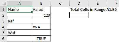
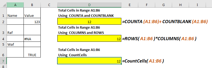
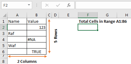
Suppose, I want to to count total number of cells in range A1:B6. We can see that it has 12 cells. Now let’s use the above formula for counting the cell in given range.

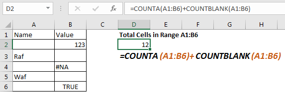
=COUNTA(A1:B6)+COUNTBLANK(A1:B6)

This formula to get cell count in range returns the correct answer.
0038
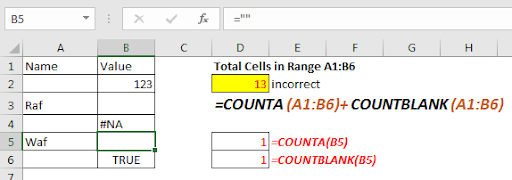
The problem: If you read about COUNTA function, you’ll find that it counts any cell containing anything, even a formula that returns blank. COUNTBLANK function also counts any cell which is blank, even if it is returned by a formula. Now since both functions will count same cells, the returned value will be incorrect. So, use this formula to count cells, when you are sure that no formula returns blank value.
0039
Count cells in a range using ROWS and COLUMN Function
Now, we all know that a range is made of rows and columns. Any range has at least one column and one row. So, if we multiply rows with columns, we will get our number of cell in excel range. This is same as we used to calculate the area of a rectangle.
0040
Generic Formula to Count Cells

=ROWS(range)*COLUMNS(range)

Let’s implement this formula in above range to count cells.

=ROWS(A1:B6)*COLUMNS(A1:B6)

0041
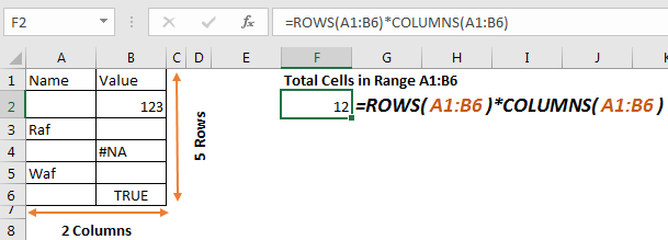
This returns the accurate number of cells in range a1:B6. It doesn’t matter what values these cells hold.
How it works
It is simple. The ROWS function, returns count of rows in range, which is 6 in this case. Similarly, COLUMN function returns the number of columns in the range, which is 2 in this example. The formula multiplies and returns the final result as 12.
CountCells VBA Function to Count All Cells in a Range
In both of the above methods, we had to use two function of excel, and provide the same range twice. This can lead to be human error. So we can define a user defined function to count cells in a range. This is easy.
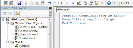
Press ALT+F11 to open VBA editor. Go to insert and click on module. Now copy below VBA code in that module.

Function CountCells(rng As Range)
CountCells = rng.CountLarge
End Function

Return to your excel file. Write CountCells function to count cells in a range. Provide range in parameter. The function will return the number of cell in the given range.

Let’s take the same example.

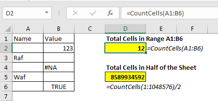
Write below formula to count cells in range A1:B6

=CountCells(A1:B6)

0042
How it works

Actually, CountLarge is method of range object that counts the cell in a given range. CountCells function takes the range from user as argument and returns the cell count in range using Range.CountLarge.
0044
This method is faster and easy to use. Once you define this function for counting cells in a range in excel, you can use it as many times as you want.

So yeah, these are the formulas to count cells in a range in excel. If you know any other ways, let us know in the comments section below.

Related Articles:

How to Count Cells that contain specific text in Excel

How to Count Unique Values In Excel

How to use the COUNT Function in Excel

How to Count Cells With Text in Excel

How to use the COUNTIFS Function in Excel

How to use the COUNTIF function in Excel

Get the Count of table rows & columns in Excel

Popular Articles :

50 Excel Shortcut to Increase Your Productivity : Get faster at your task. These 50 shortcuts will make you work even faster on Excel.

How to use the VLOOKUP Function in Excel : This is one of the most used and popular functions of excel that is used to lookup value from different ranges and sheets.

How to use the COUNTIF function in Excel : Count values with conditions using this amazing function. You don’t need to filter your data to count specific values. Countif function is essential to prepare your dashboard.

How to use the SUMIF Function in Excel : This is another dashboard essential function. This helps you sum up values on specific conditions.

Источник

This tutorial shows how to count the total number of rows from a selected range through the use of an Excel formula or VBA

METHOD 1. Count number of rows in a range

METHOD 1. Count number of rows in a range using VBA

Explanation about the formula used to count number of rows in a range

How to Count the Number of Rows in Excel?

Table of contents

#1 – Excel Count Rows which has only the Data

#2 – Count all the rows that have the data

#3 – Count the rows that only have the numbers

#4 – Count Rows, which only has the Blanks

#5 – Count rows that only have text values

#6 – Count all of the rows in the range

Things to Remember

Recommended Articles

Свойство Range.Rows (Excel)

Синтаксис

Замечания

Пример

Поддержка и обратная связь

Count Rows in Excel

How to Count the Number of Rows in Excel?

Table of contents

#1 – Excel Count Rows which has only the Data

#2 – Count all the rows that have the data

#3 – Count the rows that only have the numbers

#4 – Count Rows, which only has the Blanks

#5 – Count rows that only have text values

#6 – Count all of the rows in the range

Things to Remember

Recommended Articles

VBA – Count the rows in a Selection

Count Rows in a Selection

Count Columns in a Selection

VBA Coding Made Easy

VBA Code Examples Add-in

VBA Code Generator

AutoMacro: VBA Add-in with Hundreds of Ready-To-Use VBA Code Examples & much more!

What is AutoMacro?

Ways to count values in a worksheet

Download our examples

In this article

Simple counting

Video: Count cells by using the Excel status bar

Use AutoSum

Add a Subtotal row

Count cells in a list or Excel table column by using the SUBTOTAL function

Counting based on one or more conditions

Video: Use the COUNT, COUNTIF, and COUNTA functions

Count cells in a range by using the COUNT function

Count cells in a range based on a single condition by using the COUNTIF function

Count cells in a column based on single or multiple conditions by using the DCOUNT function

Count cells in a range based on multiple conditions by using the COUNTIFS function

Count based on criteria by using the COUNT and IF functions together

Count how often multiple text or number values occur by using the SUM and IF functions together

Count cells in a column or row in a PivotTable

Counting when your data contains blank values

Count nonblank cells in a range by using the COUNTA function

Count nonblank cells in a list with specific conditions by using the DCOUNTA function

Count blank cells in a contiguous range by using the COUNTBLANK function

Count blank cells in a non-contiguous range by using a combination of SUM and IF functions

Counting unique occurrences of values

Count the number of unique values in a list column by using Advanced Filter

Count the number of unique values in a range that meet one or more conditions by using IF, SUM, FREQUENCY, MATCH, and LEN functions

Special cases (count all cells, count words)

Count the total number of cells in a range by using ROWS and COLUMNS functions

Count words in a range by using a combination of SUM, IF, LEN, TRIM, and SUBSTITUTE functions

Displaying calculations and counts on the status bar

Need more help?

Introduction to Row Count in Excel

How to Count the Rows in Excel?

Example #1

Example #2

Example #3

Example #4

Example #5

Example #6

Things to Remember About Row Count in Excel

Recommended Articles