Excel countifs with dates

To count numbers or dates that meet a single condition (such as equal to, greater than, less than, greater than or equal to, or less than or equal to), use the COUNTIF function. To count numbers or dates that fall within a range (such as greater than 9000 and at the same time less than 22500), you can use the COUNTIFS function. Alternately, you can use SUMPRODUCT too.

Example

Note: You’ll need to adjust these cell formula references outlined here based on where and how you copy these examples into the Excel sheet.

1	A	B
2	Salesperson	Invoice
3	Buchanan	15,000
4	Buchanan	9,000
5	Suyama	8,000
6	Suyma	20,000
7	Buchanan	5,000
8	Dodsworth	22,500
9	Formula	Description (Result)
10	=COUNTIF(B2:B7,»>9000″)	The COUNTIF function counts the number of cells in the range B2:B7 that contain numbers greater than 9000 (4)
11	=COUNTIF(B2:B7,»<=9000″)	The COUNTIF function counts the number of cells in the range B2:B7 that contain numbers less than 9000 (4)
12	=COUNTIFS(B2:B7,»>=9000″,B2:B7,»<=22500″)	The COUNTIFS function (available in Excel 2007 and later) counts the number of cells in the range B2:B7 greater than or equal to 9000 and are less than or equal to 22500 (4)
13	=SUMPRODUCT((B2:B7>=9000)*(B2:B7<=22500))	The SUMPRODUCT function counts the number of cells in the range B2:B7 that contain numbers greater than or equal to 9000 and less than or equal to 22500 (4). You can use this function in Excel 2003 and earlier, where COUNTIFS is not available.
14	Date
15	3/11/2011
16	1/1/2010
17	12/31/2010
18	6/30/2010
19	Formula	Description (Result)
20	=COUNTIF(B14:B17,»>3/1/2010″)	Counts the number of cells in the range B14:B17 with a data greater than 3/1/2010 (3)
21	=COUNTIF(B14:B17,»12/31/2010″)	Counts the number of cells in the range B14:B17 equal to 12/31/2010 (1). The equal sign is not needed in the criteria, so it is not included here (the formula will work with an equal sign if you do include it («=12/31/2010»).
22	=COUNTIFS(B14:B17,»>=1/1/2010″,B14:B17,»<=12/31/2010″)	Counts the number of cells in the range B14:B17 that are between (inclusive) 1/1/2010 and 12/31/2010 (3).
23	=SUMPRODUCT((B14:B17>=DATEVALUE(«1/1/2010»))*(B14:B17<=DATEVALUE(«12/31/2010»)))	Counts the number of cells in the range B14:B17 that are between (inclusive) 1/1/2010 and 12/31/2010 (3). This example serves as a substitute for the COUNTIFS function that was introduced in Excel 2007. The DATEVALUE function converts the dates to a numeric value, which the SUMPRODUCT function can then work with.

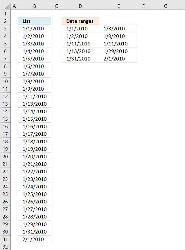
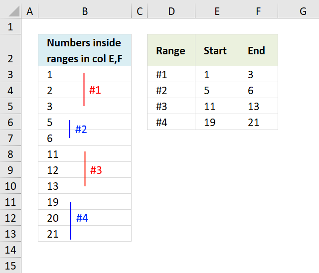
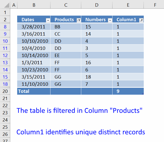
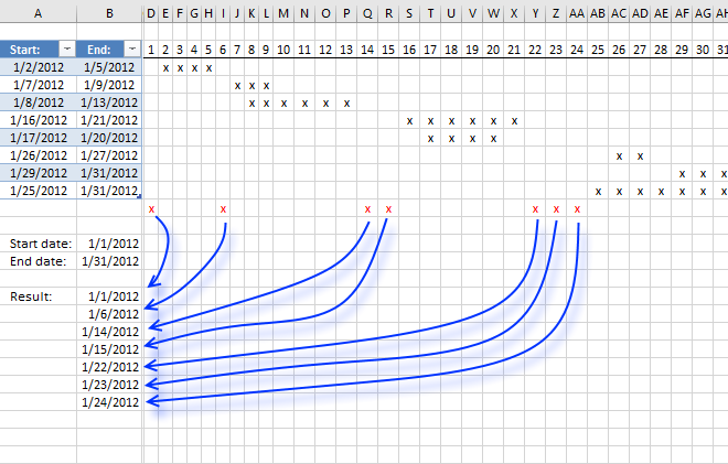
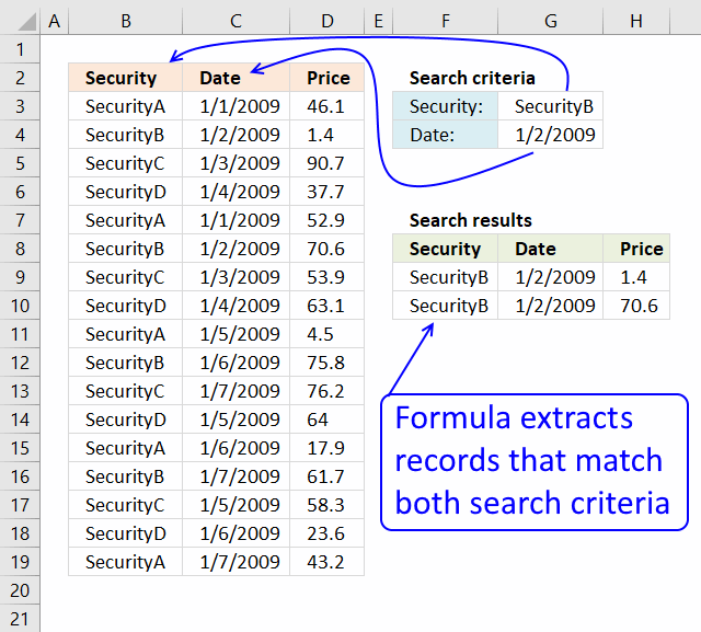
In this example, the goal is to count the number of cells in column D that contain dates that are between two variable dates in G4 and G5. This problem can be solved with the COUNTIFS function or the SUMPRODUCT function, as explained below. For convenience, the worksheet contains two named ranges: date (D5:D16) and amount (C5:C16). The named range amount is not used to count dates, but can be used to sum amounts between the same dates, as seen below.

Note: Excel dates are large serial numbers so, at the core, this problem is about counting numbers that fall into a specific range. In other words, SUMIFS and SUMPRODUCT don’t care about the dates, they only care about the numbers underneath the dates. If you like, you can see the numbers underneath by temporarily formatting the dates with the General number format.

COUNTIFS function

The COUNTIFS function is designed to count cells that meet multiple conditions. In this case, we need to provide two conditions: (1) the date is greater than or equal to G4 and (2) the date is less than or equal to G5. COUNTIFS accepts conditions as range/criteria pairs, so the conditions are entered like this:

date,">="&G4 // greater than or equal to G4
date,"<="&G5 // less than or equal to G5

The final formula looks like this:

=COUNTIFS(date,">="&G4,date,"<="&G5)

Note that the logical operators «>=» and «<=» must be entered as text and surrounded by double quotes. This means we must use concatenation with the ampersand operator (&) to join the operators to the dates in cell G4 and cell G5. This syntax is specific to a group of eight functions in Excel.

SUMPRODUCT function

This problem can also be solved with the SUMPRODUCT function which allows a cleaner syntax:

=SUMPRODUCT((date>=G4)*(date<=G5))

This is an example of using Boolean algebra in Excel. Because the named range date contains 12 dates, each expression inside SUMPRODUCT returns an array with 12 TRUE or FALSE values. When these two arrays are multiplied together, they return an array of 1s and 0s. After multiplication, we have:

=SUMPRODUCT({0;0;1;1;1;1;0;0;0;0;0;0})

SUMPRODUCT then returns the sum of the elements in the array, which is 4.

Sum amounts between dates

To sum the amounts on dates between G4 and G5 in this worksheet, you can use the SUMIFS function like this:

=SUMIFS(amount,date,">="&G4,date,"<="&G5)

The conditions in SUMIFS are the same as in COUNTIFS, but SUMIFS also accepts the range to sum as the first argument. The result is $630. 

To sum the amounts for dates between G4 and G5, you can use SUMPRODUCT like this:

=SUMPRODUCT((date>=G4)*(date<=G5)*amount)

Here again, the conditions are the same as the original SUMPRODUCT formula above, but we have extended the formula to multiply by amount. This formula simplifies to:

=SUMPRODUCT({0;0;1;1;1;1;0;0;0;0;0;0}*{180;120;105;100;220;205;225;140;180;200;240;235})

The zeros in the first array effectively cancel out the amounts for dates that don’t meet criteria:

=SUMPRODUCT({0;0;105;100;220;205;0;0;0;0;0;0})

and SUMPRODUCT returns $630 as a final result.

» » operator surrounded by double quotes («»). For example, the formula below will count cells not equal to «red» in the range A1:A10:

Blank cells

COUNTIFS can count cells that are blank or not blank. The formulas below count blank and not blank cells in the range A1:A10:

Dates

The easiest way to use COUNTIFS with dates is to refer to a valid date in another cell with a cell reference. For example, to count cells in A1:A10 that contain a date greater than a date in B1, you can use a formula like this:

Notice we concatenate the «>» operator to the date in B1, but and are no quotes around the cell reference.

The safest way to hardcode a date into COUNTIFS is with the DATE function. This guarantees Excel will understand the date. To count cells in A1:A10 that contain a date less than September 1, 2020, you can use:

Wildcards

The wildcard characters question mark (?), asterisk(*), or tilde (

) can be used in criteria. A question mark (?) matches any one character, and an asterisk (*) matches zero or more characters of any kind. For example, to count cells in A1:A5 that contain the text «apple» anywhere, you can use a formula like this:

) is an escape character to allow you to find literal wildcards. For example, to count a literal question mark (?), asterisk(*), or tilde (

), add a tilde in front of the wildcard (i.e.

OR logic

The COUNTIFS function is designed to apply multiple criteria, but conditions are applied with AND logic. This means if you try to count cells that contain «red» or «blue» in the same range, the result will be zero (0). However, to count cells with OR logic, you can use an array constant and the SUM function like this:

The formula above will count cells in range that contain «red» or «blue». Briefly, COUNTIFS returns two counts in an array (one for «red» and one for «blue») and the SUM function returns the sum as a final result. For more information, see this example.

Limitations

The COUNTIFS function has some limitations you should be aware of:

• Conditions in COUNTIFS are joined by AND logic. In other words, all conditions must be TRUE in order for a cell to be included in a count. The workaround above can be used in simple situations.
• The COUNTIFS function requires actual ranges for all range arguments; you can’t use an array. This means you can’t alter values that appear in a range argument before applying criteria.
• COUNTIFS is not case-sensitive. To count values based on a case-sensitive condition, you can use a formula based on the SUMPRODUCT function with the EXACT function.
• COUNTIFS has some other quirks, which are detailed in this article.

The most common way to work around the limitations above is to use the SUMPRODUCT function. In the current version of Excel, another option is to use the newer BYROW and BYCOL functions.

Источник

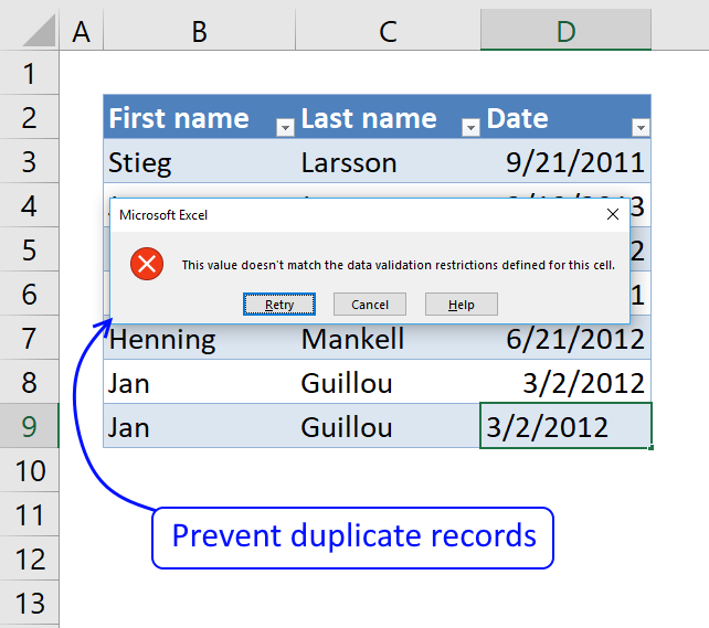
How to count cells between two dates using COUNTIFS

You can use the COUNTIFS function to count the number of cells between two dates of an Excel file. In this example, the COUNTIF function isn’t suitable because you cannot use COUNTIF for multiple criteria, and we want to count the number of Excel records that fall between two dates.

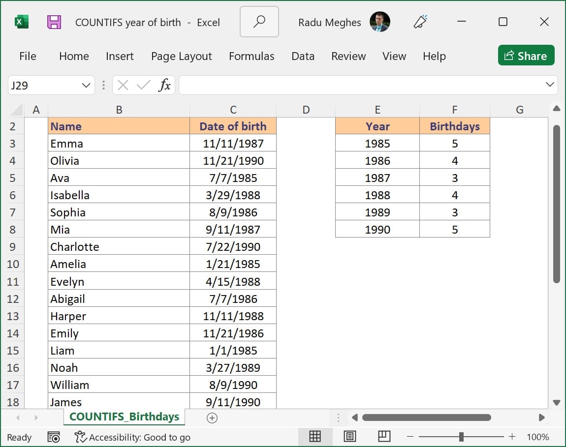
Step by step COUNTIFS formula with two dates

1. Type =COUNTIFS(
2. Select or type the range reference for criteria_range1. In my example, I used a named range: Birthday.
3. Insert criteria1. I wanted to count all birth dates after January 1st, 1985, so I inserted “>=”&DATE(E3,1,1) where cell E3 contains the year 1985.
4. Select your date range again. Since we want to apply two criteria for the same data set, you will need to select the same range again.
5. Insert criteria2, which is the maximum date we are interested in. In my case, I wanted to count the birth dates which occurred during 1985, which means a maximum date of December 31st, 1985, so I used » .
6. Type ) and then press Enter to complete the COUNTIFS formula.

COUNTIFS with dates – The Excel syntax

COUNTIFS(criteria_range1, criteria1, [criteria_range2, criteria2]…)

where:
criteria_range1 – the first range to compare against your criteria (Required)
criteria1 – The criteria to use on range1. It can be a number, expression, cell reference, or text that defines which cells are counted (Required)
criteria_range2 – the second range to compare against your criteria (Optional)
criteria2 – The criteria to use on range2. It can be a number, expression, cell reference, or text that defines which cells are counted (Optional)

In our example, cell F3 contains the following formula to count if the date is between two dates:
=COUNTIFS(Birthday, «>=»&DATE(E3,1,1), Birthday, «

How to use this COUNTIFS formula with multiple criteria

Since we need to check for two conditions, the COUNTIFS function is appropriate because this Excel function can easily count the number of entries between two cell values. To add the date, you can either select it from a cell or create it using the DATE function as I did below.

The first condition in cell F3 Birthday,»>=»&DATE(E3,1,1) checks if the birth date in the COUNTIFS date range is greater than or equal to January 1st, 1985, while the second one Birthday,» checks if the birth date is less than or equal to December 31st, 1985. The COUNTIFS function will return the number of cells that have dates between the two specified days if both COUNTIFS criteria are met.

When using COUNTIFS with dates, it’s important to remember to use the same COUNTIFS date range. Please note that the range “Birthday” contains cells C3:C26 from the table. This means that you need to use the same cell reference for both criteria, or else Excel will return the #VALUE! error message.

Since the logical operators «>=» and » need to be entered as text between double quotes, we have to use the symbol & to concatenate the operator with each date. If you skip this step, Excel will not be able to understand your formula and will display an error message.

The following formula counts the cells between two dates by referencing the cells directly, without using the DATE function. I’ve used the same conditions: «>=»&E3 and » and the result is the same as in the previous example.

You can also use this formula to count cells between two numbers in the same way you are using COUNTIFS with two dates.

What to do next?

If you still struggle and have additional questions about how to use COUNTIFS with date ranges and multiple criteria, please let me know by posting a comment.

About me

My name is Radu Meghes, and I’m the owner of excelexplained.com. Over the past 15+ years, I have been using Microsoft Excel in my day-to-day job. I’ve worked as an investment and business analyst, and Excel has always been my most powerful weapon. Its flexibility and complexity make it a highly demanded skill for finance employees. I launched excelexplained.com back in 2017, and it has become a trusted source for Excel tutorials for hundreds of thousands of people each year.

If you’d like to get in touch, you can contact me on LinkedIn.

Источник

How to Use Multiple Criteria in Excel COUNTIF and COUNTIFS Function

Excel has many functions where a user needs to specify a single or multiple criteria to get the result. For example, if you want to count cells based on multiple criteria, you can use the COUNTIF or COUNTIFS functions in Excel.

This tutorial covers various ways of using a single or multiple criteria in COUNTIF and COUNTIFS function in Excel.

While I will primarily be focussing on COUNTIF and COUNTIFS functions in this tutorial, all these examples can also be used in other Excel functions that take multiple criteria as inputs (such as SUMIF, SUMIFS, AVERAGEIF, and AVERAGEIFS).

This Tutorial Covers:

An Introduction to Excel COUNTIF and COUNTIFS Functions

Let’s first get a grip on using COUNTIF and COUNTIFS functions in Excel.

Excel COUNTIF Function (takes Single Criteria)

Excel COUNTIF function is best suited for situations when you want to count cells based on a single criterion. If you want to count based on multiple criteria, use COUNTIFS function.

Syntax

Input Arguments

• range – the range of cells which you want to count.
• criteria – the criteria that must be evaluated against the range of cells for a cell to be counted.

Excel COUNTIFS Function (takes Multiple Criteria)

Excel COUNTIFS function is best suited for situations when you want to count cells based on multiple criteria.

Syntax

= COUNTIFS(cr iteria_range1, criteria1, [criteria_range2, criteria2]…)

Input Arguments

• criteria_range1 – The range of cells for which you want to evaluate against criteria1.
• criteria1 – the criteria which you want to evaluate for criteria_range1 to determine which cells to count.
• [criteria_range2] – The range of cells for which you want to evaluate against criteria2.
• [criteria2] – the criteria which you want to evaluate for criteria_range2 to determine which cells to count.

Now let’s have a look at some examples of using multiple criteria in COUNTIF functions in Excel.

Using NUMBER Criteria in Excel COUNTIF Functions

#1 Count Cells when Criteria is EQUAL to a Value

To get the count of cells where the criteria argument is equal to a specified value, you can either directly enter the criteria or use the cell reference that contains the criteria.

Below is an example where we count the cells that contain the number 9 (which means that the criteria argument is equal to 9). Here is the formula:

In the above example (in the pic), the criteria is in cell D3. You can also enter the criteria directly into the formula. For example, you can also use:

#2 Count Cells when Criteria is GREATER THAN a Value

To get the count of cells with a value greater than a specified value, we use the greater than operator (“>”). We could either use it directly in the formula or use a cell reference that has the criteria.

Whenever we use an operator in criteria in Excel, we need to put it within double quotes. For example, if the criteria is greater than 10, then we need to enter “>10” as the criteria (see pic below):

Here is the formula:

You can also have the criteria in a cell and use the cell reference as the criteria. In this case, you need NOT put the criteria in double quotes:

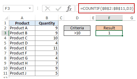
There could also be a case when you want the criteria to be in a cell, but don’t want it with the operator. For example, you may want the cell D3 to have the number 10 and not >10.

In that case, you need to create a criteria argument which is a combination of operator and cell reference (see pic below):

NOTE: When you combine an operator and a cell reference, the operator is always in double quotes. The operator and cell reference are joined by an ampersand (&).

#3 Count Cells when Criteria is LESS THAN a Value

To get the count of cells with a value less than a specified value, we use the less than operator (“ =COUNTIF($B$2:$B$11,”

You can also have the criteria in a cell and use the cell reference as the criteria. In this case, you need NOT put the criteria in double quotes (see pic below):

Also, there could be a case when you want the criteria to be in a cell, but don’t want it with the operator. For example, you may want the cell D3 to have the number 5 and not =COUNTIF($B$2:$B$11,”

NOTE: When you combine an operator and a cell reference, the operator is always in double quotes. The operator and cell reference are joined by an ampersand (&).

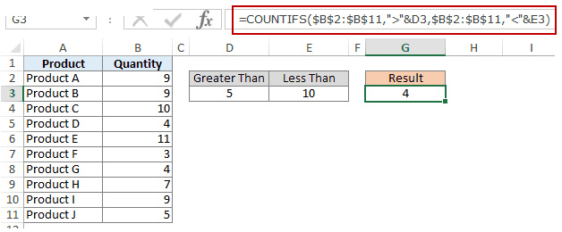
#4 Count Cells with Multiple Criteria – Between Two Values

To get a count of values between two values, we need to use multiple criteria in the COUNTIF function.

Here are two methods of doing this:

METHOD 1: Using COUNTIFS function

COUNTIFS function can handle multiple criteria as arguments and counts the cells only when all the criteria are TRUE. To count cells with values between two specified values (say 5 and 10), we can use the following COUNTIFS function:

NOTE: The above formula does not count cells that contain 5 or 10. If you want to include these cells, use greater than equal to (>=) and less than equal to ( =COUNTIFS($B$2:$B$11,”>=5″,$B$2:$B$11,”

You can also have these criteria in cells and use the cell reference as the criteria. In this case, you need NOT put the criteria in double quotes (see pic below):

You can also use a combination of cells references and operators (where the operator is entered directly in the formula). When you combine an operator and a cell reference, the operator is always in double quotes. The operator and cell reference are joined by an ampersand (&).

METHOD 2: Using two COUNTIF functions

If you have multiple criteria, you can either use COUNTIFS or create a combination of COUNTIF functions. The formula below would also do the same thing:

In the above formula, we first find the number of cells that have a value greater than 5 and we subtract the count of cells with a value greater than 10. This would give us the result as 5 (which is the number of cells that have values more than 5 and less than equal to 10).

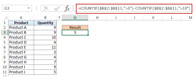
If you want the formula to include both 5 and 10, use the following formula instead:

If you want the formula to exclude both ‘5’ and ’10’ from the counting, use the following formula:

You can have these criteria in cells and use the cells references, or you can use a combination of operators and cells references.

Using TEXT Criteria in Excel Functions

#1 Count Cells when Criteria is EQUAL to a Specified text

To count cells that contain an exact match of the specified text, we can simply use that text as the criteria. For example, in the dataset (shown below in the pic), if I want to count all the cells with the name Joe in it, I can use the below formula:

Since this is a text string, I need to put the text criteria in double quotes.

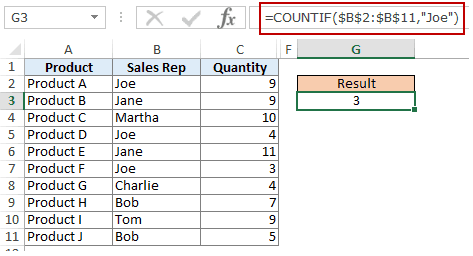
You can also have the criteria in a cell and then use that cell reference (as shown below):

NOTE: You can get wrong results if there are leading/trailing spaces in the criteria or criteria range. Make sure you clean the data before using these formulas.

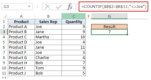
#2 Count Cells when Criteria is NOT EQUAL to a Specified text

Similar to what we saw in the above example, you can also count cells that do not contain a specified text. To do this, we need to use the not equal to operator (<>).

Suppose you want to count all the cells that do not contain the name JOE, here is the formula that will do it:

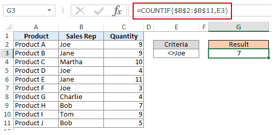
You can also have the criteria in a cell and use the cell reference as the criteria. In this case, you need NOT put the criteria in double quotes (see pic below):

There could also be a case when you want the criteria to be in a cell but don’t want it with the operator. For example, you may want the cell D3 to have the name Joe and not <>Joe.

In that case, you need to create a criteria argument which is a combination of operator and cell reference (see pic below):

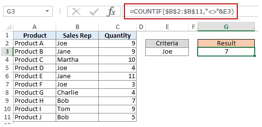
When you combine an operator and a cell reference, the operator is always in double quotes. The operator and cell reference are joined by an ampersand (&).

Using DATE Criteria in Excel COUNTIF and COUNTIFS Functions

Excel store date and time as numbers. So we can use it the same way we use numbers.

#1 Count Cells when Criteria is EQUAL to a Specified Date

To get the count of cells that contain the specified date, we would use the equal to operator (=) along with the date.

To use the date, I recommend using the DATE function, as it gets rid of any possibility of error in the date value. So, for example, if I want to use the date September 1, 2015, I can use the DATE function as shown below:

This formula would return the same date despite regional differences. For example, 01-09-2015 would be September 1, 2015 according to the US date syntax and January 09, 2015 according to the UK date syntax. However, this formula would always return September 1, 2105.

Here is the formula to count the number of cells that contain the date 02-09-2015:

#2 Count Cells when Criteria is BEFORE or AFTER to a Specified Date

To count cells that contain date before or after a specified date, we can use the less than/greater than operators.

For example, if I want to count all the cells that contain a date that is after September 02, 2015, I can use the formula:

Similarly, you can also count the number of cells before a specified date. If you want to include a date in the counting, use and ‘equal to’ operator along with ‘greater than/less than’ operator.

You can also use a cell reference that contains a date. In this case, you need to combine the operator (within double quotes) with the date using an ampersand (&).

See example below:

#3 Count Cells with Multiple Criteria – Between Two Dates

To get a count of values between two values, we need to use multiple criteria in the COUNTIF function.

We can do this using two methods – One single COUNTIFS function or two COUNTIF functions.

METHOD 1: Using COUNTIFS function

COUNTIFS function can take multiple criteria as the arguments and counts the cells only when all the criteria are TRUE. To count cells with values between two specified dates (say September 2 and September 7), we can use the following COUNTIFS function:

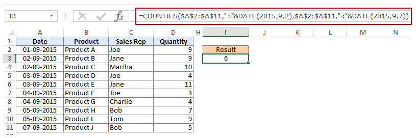
The above formula does not count cells that contain the specified dates. If you want to include these dates as well, use greater than equal to (>=) and less than equal to ( =COUNTIFS($A$2:$A$11,”>=”&DATE(2015,9,2),$A$2:$A$11,”

You can also have the dates in a cell and use the cell reference as the criteria. In this case, you can not have the operator with the date in the cells. You need to manually add operators in the formula (in double quotes) and add cell reference using an ampersand (&). See the pic below:

METHOD 2: Using COUNTIF functions

If you have multiple criteria, you can either use one COUNTIFS function or create a combination of two COUNTIF functions. The formula below would also do the trick:

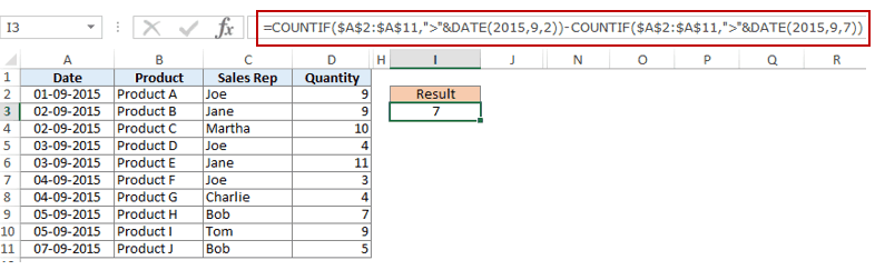
In the above formula, we first find the number of cells that have a date after September 2 and we subtract the count of cells with dates after September 7. This would give us the result as 7 (which is the number of cells that have dates after September 2 and on or before September 7).

If you don’t want the formula to count both September 2 and September 7, use the following formula instead:

If you want to exclude both the dates from counting, use the following formula:

Also, you can have the criteria dates in cells and use the cells references (along with operators in double quotes joined using ampersand).

Using WILDCARD CHARACTERS in Criteria in COUNTIF & COUNTIFS Functions

1. * (asterisk) – It represents any number of characters. For example, ex* could mean excel, excels, example, expert, etc.
2. ? (question mark) – It represents one single character. For example, Tr?mp could mean Trump or Tramp.

(tilde) – It is used to identify a wildcard character (

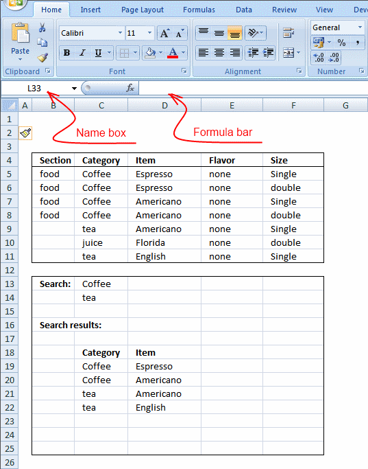
You can use COUNTIF function with wildcard characters to count cells when other inbuilt count function fails. For example, suppose you have a data set as shown below:

Now let’s take various examples:

#1 Count Cells that contain Text

To count cells with text in it, we can use the wildcard character * (asterisk). Since asterisk represents any number of characters, it would count all cells that have any text in it. Here is the formula:

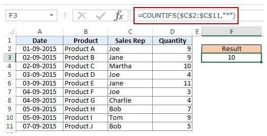
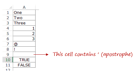
Note: The formula above ignores cells that contain numbers, blank cells, and logical values, but would count the cells contain an apostrophe (and hence appear blank) or cells that contain empty string (=””) which may have been returned as a part of a formula.

Here is a detailed tutorial on handling cases where there is an empty string or apostrophe.

Here is a detailed tutorial on handling cases where there are empty strings or apostrophes.

Below is a video that explains different scenarios of counting cells with text in it.

#2 Count Non-blank Cells

If you are thinking of using COUNTA function, think again.

Try it and it might fail you. COUNTA will also count a cell that contains an empty string (often returned by formulas as =”” or when people enter only an apostrophe in a cell). Cells that contain empty strings look blank but are not, and thus counted by the COUNTA function.

COUNTA will also count a cell that contains an empty string (often returned by formulas as =”” or when people enter only an apostrophe in a cell). Cells that contain empty strings look blank but are not, and thus counted by the COUNTA function.

So if you use the formula = COUNTA (A1:A11) , it returns 11, while it should return 10.

Here is the fix:

Let’s understand this formula by breaking it down:

#3 Count Cells that contain specific text

Let’s say we want to count all the cells where the sales rep name begins with J. This can easily be achieved by using a wildcard character in COUNTIF function. Here is the formula:

The criteria J* specifies that the text in a cell should begin with J and can contain any number of characters.

If you want to count cells that contain the alphabet anywhere in the text, flank it with an asterisk on both sides. For example, if you want to count cells that contain the alphabet “a” in it, use *a* as the criteria.

This article is unusually long compared to my other articles. Hope you have enjoyed it. Let me know your thoughts by leaving a comment.

You May Also Find the following Excel tutorials useful:

Источник

Adblock
detector

You can use the COUNTIFS function to count the number of cells between two dates of an Excel file. In this example, the COUNTIF function isn’t suitable because you cannot use COUNTIF for multiple criteria, and we want to count the number of Excel records that fall between two dates.

Step by step COUNTIFS formula with two dates

1. Type =COUNTIFS(
2. Select or type the range reference for criteria_range1. In my example, I used a named range: Birthday.
3. Insert criteria1. I wanted to count all birth dates after January 1st, 1985, so I inserted “>=”&DATE(E3,1,1) where cell E3 contains the year 1985.
4. Select your date range again. Since we want to apply two criteria for the same data set, you will need to select the same range again.
5. Insert criteria2, which is the maximum date we are interested in. In my case, I wanted to count the birth dates which occurred during 1985, which means a maximum date of December 31st, 1985, so I used "<="&DATE(E3,12,31).
6. Type ) and then press Enter to complete the COUNTIFS formula.

COUNTIFS with dates – The Excel syntax

COUNTIFS(criteria_range1, criteria1, [criteria_range2, criteria2]…)

where:
criteria_range1 – the first range to compare against your criteria (Required)
criteria1 – The criteria to use on range1. It can be a number, expression, cell reference, or text that defines which cells are counted (Required)
criteria_range2 – the second range to compare against your criteria (Optional)
criteria2 – The criteria to use on range2. It can be a number, expression, cell reference, or text that defines which cells are counted (Optional)

In our example, cell F3 contains the following formula to count if the date is between two dates:
=COUNTIFS(Birthday, ">="&DATE(E3,1,1), Birthday, "<="&DATE(E3,12,31))

How to use this COUNTIFS formula with multiple criteria

Since we need to check for two conditions, the COUNTIFS function is appropriate because this Excel function can easily count the number of entries between two cell values. To add the date, you can either select it from a cell or create it using the DATE function as I did below.

The first condition in cell F3 Birthday,">="&DATE(E3,1,1) checks if the birth date in the COUNTIFS date range is greater than or equal to January 1st, 1985, while the second one Birthday,"<="&DATE(E3,12,31) checks if the birth date is less than or equal to December 31st, 1985. The COUNTIFS function will return the number of cells that have dates between the two specified days if both COUNTIFS criteria are met.

When using COUNTIFS with dates, it’s important to remember to use the same COUNTIFS date range. Please note that the range “Birthday” contains cells C3:C26 from the table. This means that you need to use the same cell reference for both criteria, or else Excel will return the #VALUE! error message.

Since the logical operators ">=" and "<=" need to be entered as text between double quotes, we have to use the symbol & to concatenate the operator with each date. If you skip this step, Excel will not be able to understand your formula and will display an error message.

The following formula counts the cells between two dates by referencing the cells directly, without using the DATE function. I’ve used the same conditions: ">="&E3 and "<="&F3 and the result is the same as in the previous example.

You can also use this formula to count cells between two numbers in the same way you are using COUNTIFS with two dates.

What to do next?

In this article, I’ve shown you two examples of how to count cells between two dates using the COUNTIFS function. While this can be useful at your job, I encourage you to learn more by reading some of the following articles:

• How to count cells equal to a specific value
• How to sum sales by year
• How to separate first and last name
• How to count cells that contain odd numbers
• How to subtotal by item type
• How to use an IF function with multiple conditions

If you still struggle and have additional questions about how to use COUNTIFS with date ranges and multiple criteria, please let me know by posting a comment.

There are a handful of functions that we can use to count by date, month, year, or date range in Excel 365.

We can use Excel functions such as COUNTIF, COUNTIFS, SUMPRODUCT, or combinations such as IF + SUM or COUNT + FILTER for this.

But I would pick the former two functions in Excel 365. Do you know why?

Dynamic array formulas, which spill results, are one of the main attractions in Excel in Microsoft 365.

If you are looking for a dynamic array formula to count by date, month, year, and date range in Excel 365, pick none other than COUNTIF/COUNTIFS.

So, in this tutorial, let’s learn to use COUNTIF or COUNTIFS to count by date, month, year, and date range and return an array result.

Sample Records

I have extracted a few records from my daily expense spreadsheet.

Of course, I have sanitized the data to avoid sharing personal info/preferences.

So it’s just a mockup of data in Excel 365. In that, we can try to use COUNTIF and COUNTIFS to count by date, month & year, month, year, and date range.

We will try conditions (criteria) in single (non-array) and multiple (array) rows.

At one instance, we will use a helper column, and that is for the count by month (not month and year).

Sample Data:

COUNTIF to Count by a Specific Date in Excel 365

Countif Syntax: COUNTIF(range,criteria)

Non-Array Formula (Single Date)

How to search and count the number of transactions on a particular date in the above records?

Criterion/Condition: 01/06/2020 (cell F2)

Formula:-

Insert the below Excel COUNTIF formula in cell G2 to count by the specific date, i.e., 01/06/2020.

=COUNTIF(A2:A22,F2)

The above Excel formula searches F2 date in A2:A22 and returns the count, i.e., 2.

Array Formula (Multiple Dates)

Can we use multiple dates (criteria) to count in the above Excel 365 formula?

Yes. Here is how.

Criteria/Conditions: 02/06/2020 (cell F4) and 01/07/2020 (cell F5).

Formula:-

Insert the below Excel COUNTIF formula in cell G4 to count by the specific dates, i.e., 02/06/2020 and 01/07/2020. It will automatically spill in G5.

=COUNTIF(A2:A22,F4:F5)

COUNTIFS to Count by Month and Year in Excel 365

COUNTIFS Syntax: COUNTIFS(criteria_range1,criteria1, ...)

The functions COUNTIF and COUNTIFS in Excel 365 won’t take other functions in their ‘range’.

So we can’t use month(range)= within these two functions.

But they support other functions in the criteria part, and we will try to benefit from that feature below.

Non-Array Formula (Month and Year)

We can use COUNTIFS to count by month and year in Excel 365.

Criterion/Condition: 6 (cell F8) and 2020 (cell G8).

Formula:-

Insert the below Excel COUNTIFS formula in cell H8 to count by the above month and year.

=COUNTIFS(A2:A22,">="&DATE(G8,F8,1),A2:A22,"<="&EOMONTH(DATE(G8,F8,1),0))

The DATE(G8,F8,1) formula returns 01/06/2020, and EOMONTH(DATE(G8,F8,1)) returns the last date in that month.

The count of dates between these dates will be equal to the count by month and year.

Array Formula (Months and Years)

We can use multiple months and years (criteria) in the above Excel 365 formula.

Criteria/Conditions:

1. 7 (cell F10) and 2020 (cell G10).
2. 7 (cell F11) and 2021 (cell G11).

Formula:-

Insert the below Excel COUNTIFS formula in cell H10 to count by the above multiple months and years.

=COUNTIFS(A2:A22,">="&DATE(G10:G11,F10:F11,1),A2:A22,"<="&EOMONTH(DATE(G10:G11,F10:F11,1),0))

Array and Non-Array COUNTIFS to Count by Year in Excel 365

Assume we have the year 2020 in cell F14.

The following COUNTIFS non-array in cell G14 returns the count by the provided year in Excel 365.

=COUNTIFS(A2:A22,">="&DATE(F14,1,1),A2:A22,"<="&DATE(F14,12,31))

If the year 2020 is in cell F16 and 2021 is in cell F17, then we can use the below Excel 365 dynamic array formula in cell G16.

=COUNTIFS(A2:A22,">="&DATE(F16:F17,1,1),A2:A22,"<="&DATE(F16:F17,12,31))

I hope, the above two Excel formulas are self-explanatory. Let’s move to the next example.

Array and Non-Array COUNTIFS to Count by Date Range in Excel 365

In the above examples, we have learned to count the number of transactions that have taken place on a specific date, month, and year.

But what about counting the number of transactions between two dates in Excel 365?

I wish to know how many transactions I have done during 01/06/2020 (F20) and 06/06/2020 (G20).

I can use the below Excel formula in cell H20 for that.

Count by Date Range Non-Array Formula (H20):

=COUNTIFS(A2:A22,">="&F20,A2:A22,"<="&G20)

What about a count by date range array formula?

Date Range 1: F22:G22

Date Range 2: F23:G23

Count by Date Range Array Formula (H22):

=COUNTIFS(A2:A22,">="&F22:F23,A2:A22,"<="&G22:G23)

Array and Non-Array COUNTIFS to Count by Month Alone in Excel 365

I know this is a rare scenario.

Usually, we may include the year component in such calculations.

For example, we will usually find the number of sales in January 2020, not in both January 2020 and January 2021.

But if you are very particular to use COUNTIFS to count by month only in Excel 365, follow the below steps.

Insert the below formula in cell D2. It will substitute the year part of the dates in cell A2:A22 with the year 2021.

=DATE(2021,MONTH(A2:A22),1)

It’s a dynamic array (spill) formula. So it requires a blank range in D3:D22.

You can then hide column D or keep it.

In cell K8, enter 6 which represents June.

=COUNTIFS(D2#,">="&DATE(2021,J10,1),D2#,"<="&EOMONTH(DATE(2021,J10,1),0))

The above formula in cell L8 will return the count of transactions in June. It ignores the years!

What about an array formula?

Enter 6 in K10 and 7 in K11. Then, you may insert the below formula in L10.

=COUNTIFS(D2#,">="&DATE(2021,K10:K11,1),D2#,"<="&EOMONTH(DATE(2021,K10:K11,1),0))

Excel 365 Resources

• Running Count Array Formula in Excel 365.
• Array Formula to Conditional Count Unique Values in Excel 365.
• Split Function Alternative in Excel 365 with Multi-Row Support.
• How to Flatten an Array in Excel 365 Using Dynamic Formulas.
• Spill Formulas to Sum Each Row in Excel 365.

Author: Oscar Cronquist Article last updated on January 19, 2023

The COUNTIFS function calculates the number of cells across multiple ranges that equals all given conditions.

It allows you to use up to 254 arguments or 127 criteria pairs.

1. COUNTIFS Function Syntax

COUNTIFS(criteria_range1, criteria1, [criteria_range2, criteria2]…)

Back to top

2. COUNTIFS function Arguments

criteria_range1	Required. The cell range you want to count the cells meeting a condition.
criteria1	Required. The condition that you want to count.
[criteria_range2]	Optional. Additional ranges, up to 127 pairs.
[criteria2]	Optional. Additional ranges, up to 127 pairs.

Back to top

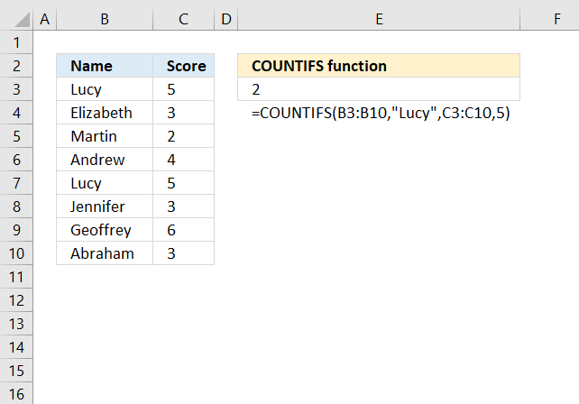
3. COUNTIFS function example

The COUNTIFS function counts the number of rows that equals one or more conditions.

Formula in cell E3:

=COUNTIFS(B3:B10,»Lucy»,C3:C10,5)

Lucy and 5 are found twice, in rows 3 and 7, the COUNTIFS function returns 2 in cell E3. All conditions must be met on the same row.

Back to top

4. COUNTIFS function — Partial match using wildcard characters

The optional wildcard characters make the COUNTIFS function even more powerful, these characters are * asterisk and question marks ? The question mark ? matches a single character while the * asterisk matches any sequence of characters even 0 (zero) characters.

Formula in cell E6:

=COUNTIFS(B3:B10, E3, C3:C10, F3)

4.1 Explaining formula

Step 1 — Populate arguments

COUNTIFS(criteria_range1, criteria1, [criteria_range2, criteria2]…)

criteria_range1 — B3:B10
criteria1 — E3
criteria_range2 — C3:C10
criteria2 — F3

COUNTIFS(B3:B10, E3, C3:C10, F3)

Step 2 — Evaluate COUNTIFS function

COUNTIFS(B3:B10, E3, C3:C10, F3)

becomes

COUNTIFS({«Lucy»; «Elizabeth»; «Martin»; «Andrew»; «Steve»; «Jennifer»; «Geoffrey»; «Abraham»}, «*n*», {«Canada»; «US»; «France»; «Spain»; «Italy»; «Canada»; «Italy»; «France»}, «*an*»)

The asterisk matches 0 (zero) to any number of characters, and a leading and trailing asterisk «*n*» matches any value that contains the character n in cells B3:B10. «Martin», «Andrew», «Jennifer» contains a «n»

«*an*» matches any country in cells C3:C10 that contains «an», they are found in rows 3, 5, 8, and 10. The COUNTIFS function counts a row if both conditions are met.

COUNTIFS({«Lucy»; «Elizabeth»; «Martin»; «Andrew»; «Steve»; «Jennifer»; «Geoffrey»; «Abraham»}, «*n*», {«Canada»; «US»; «France»; «Spain»; «Italy»; «Canada»; «Italy»; «France»}, «*an*»)

returns

2.

Back to top

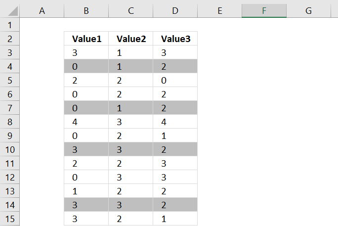
5. COUNTIFS function — using two conditions

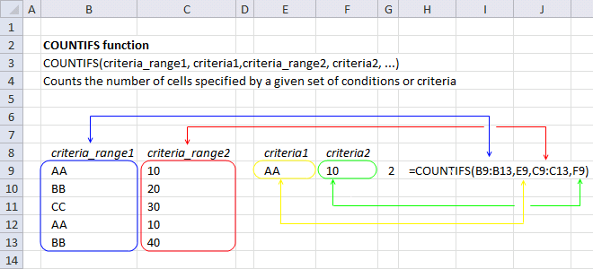
This example demonstrates the COUNTIFS function with two conditions applied to two separate columns. The COUNTIFS function counts a record when both conditions are met on the same row.

=COUNTIFS(B9:B13,E9,C9:C13,F9)

This formula checks if text string «AA» is found in cell range B9:B13 and if 10 is found in cell range C9:c13. Row 9 and 12 contain both conditions and 2 are returned to cell G9.

COUNTIFS(B9:B13,E9,C9:C13,F9)

becomes

COUNTIFS({«AA«;»BB»;»CC»;»AA«;»BB»},»AA«,{10;20;30;10;40},10)

and returns 2 in cell G9.

The calculation above shows two arrays and ou can tell that by the curly brackets {}.

The values in those arrays are separated by a semicolon meaning the values are on a row each.

Here is a post where I use this technique: Highlight duplicate rows

Back to top

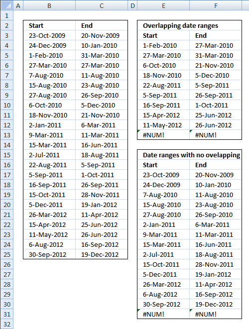
6. COUNTIFS function — Logical operators

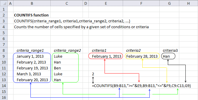
The following formula counts how many times text string «Han» equals a cell value in cell range C9:C13, it also checks if dates in cell range B9:B13 are larger than or equal to February 1st, 2013 and smaller than or equal to February 28, 2013.

=COUNTIFS(B9:B13,»>=»&E9,B9:B13,»<=»&F9,C9:C13,G9)

Three conditions in total are applied to two cell ranges, this also demonstrates that you can use logical operators with conditions. Make sure you use double quotes enclosing the logical operators and an ampersand to concatenate the values with the logical operators.

Here is a list of all logical operators you can use and their combinations.

• = equal to
• < less than
• > larger than
• <= less than or equal to
• >=larger than or equal to
• <> not equal to

COUNTIFS(B9:B13, «>=»&E9, B9:B13, «<=»&F9, C9:C13, G9)

becomes

COUNTIFS({41275; 41307; 41324; 41336; 41325}, «>=»&41306, {41275; 41307; 41324; 41336; 41325}, «<=»&41333, {«Luke»; «Han»; «Ben»; «Luke»; «Han»}, «Han»)

and returns 2 in cell E12. Row 9 and 13 have the word «Han» and are in the month of February 2013.

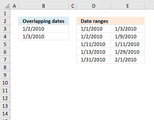
Here is a post where I use comparison operators: Filter overlapping date ranges

Back to top

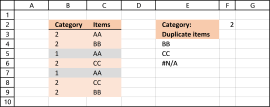
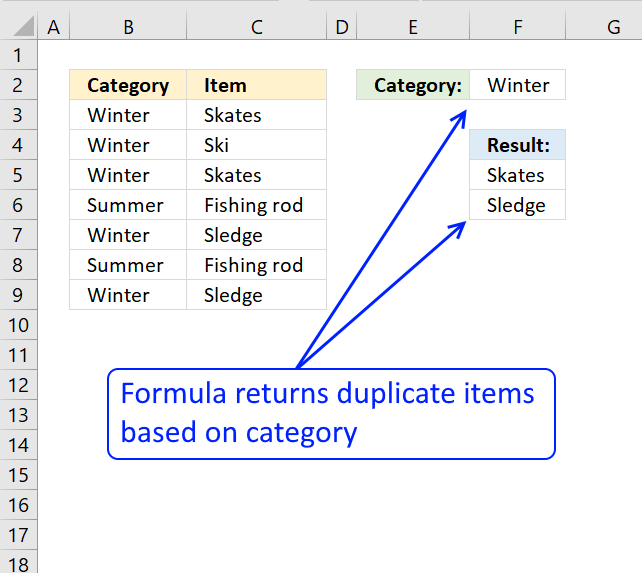
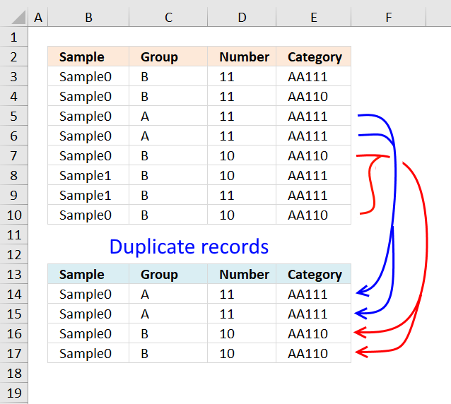
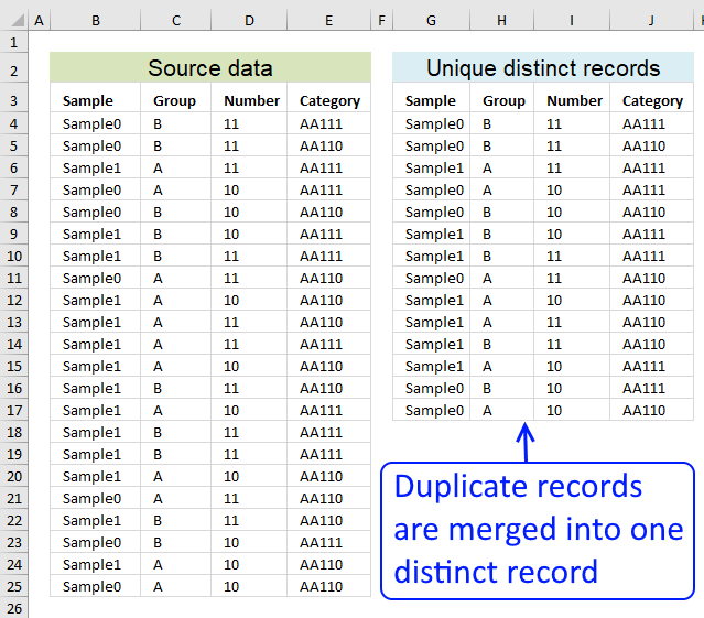
7. COUNTIFS function — Count duplicate records

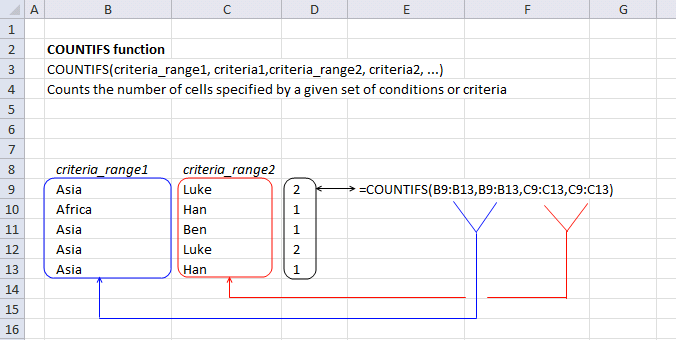
The following array formula counts each cell value in each row and returns an array of values.

=COUNTIFS(B9:B13,B9:B13,C9:C13,C9:C13)

I demonstrated in example 1 and 2 above how to use a single condition in each criteria argument, the formula above demonstrates what happens if you use multiple conditions.

Note, you will receive an error if you don’t use the same number of conditions in each criteria argument.

COUNTIFS(B9:B13, B9:B13, C9:C13, C9:C13)

becomes

COUNTIFS({«Asia»; «Africa»; «Asia»; «Asia»; «Asia»},{«Asia»; «Africa»; «Asia»; «Asia»; «Asia»},{«Luke»; «Han»; «Ben»; «Luke»; «Han»},{«Luke»; «Han»; «Ben»; «Luke»; «Han»})

and returns this array {2; 1; 1; 2; 1} in cell range D9:D13. This array is interesting because it identifies how many times each record occurs in the data set.

Here are two posts where I use this technique:

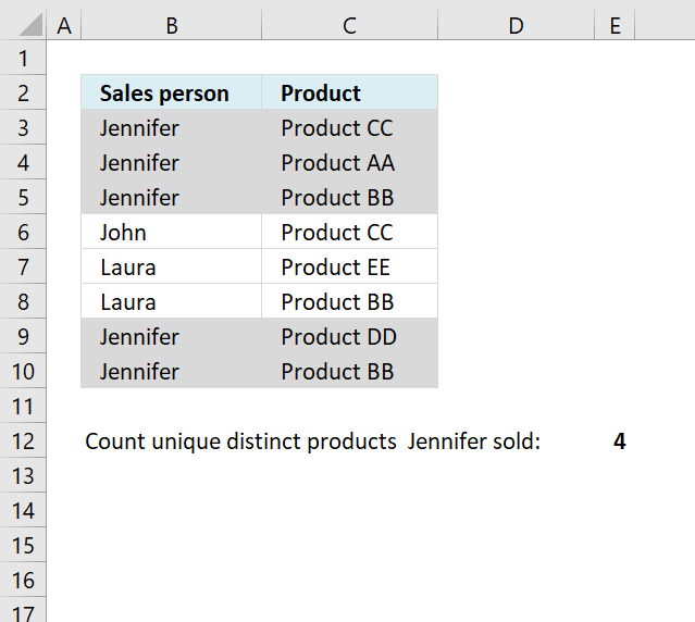
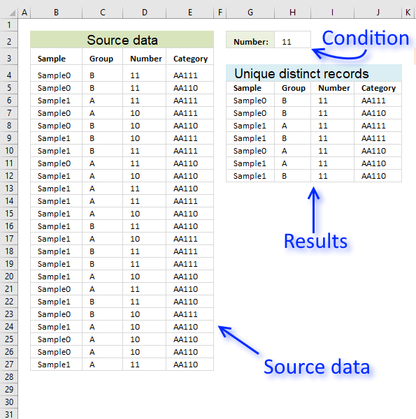
• Count unique distinct records
• Filter unique distinct row records

Back to top

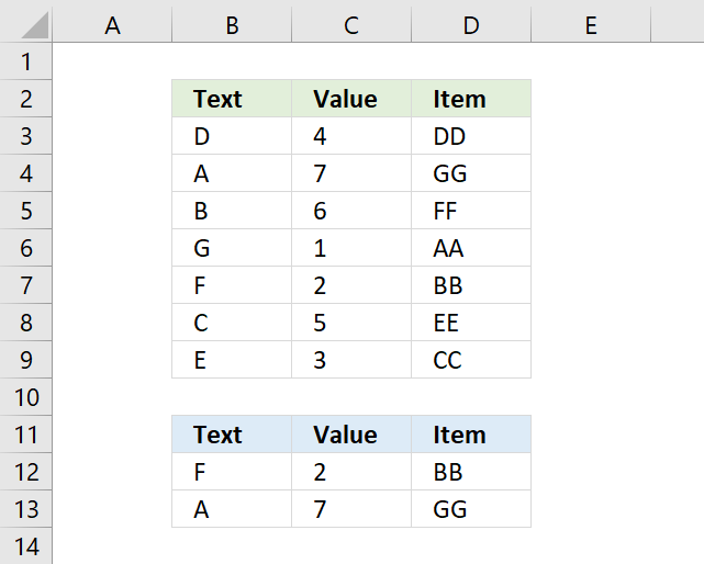
8. COUNTIFS function — return an array identifying records based on multiple conditions

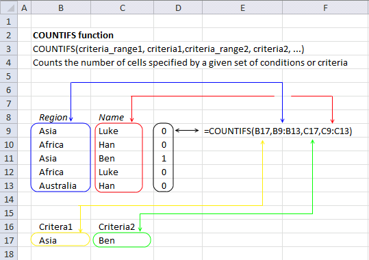
In this example, I am using a single cell value as a criteria_range argument and a cell range as criteria argument. This may seem confusing but it is definitely possible and sometimes very useful.

Array formula in cell D9:D13

=COUNTIFS(B17,B9:B13,C17,C9:C13)

8.1 How to enter an array formula

Excel 365 users can skip these steps, press Enter to enter the formula like a regular formula.

1. Select cells D9:D13.
2. Type the formula above: =COUNTIFS(B17,B9:B13,C17,C9:C13)
3. Press and hold CTRL + SHIFT simultaneously.
4. Press Enter once.
5. Release all keys.

The formula is now enclosed with curly brackets like this: {=COUNTIFS(B17,B9:B13,C17,C9:C13)}

Don’t enter these characters yourself, they appear automatically if you followed the steps above.

8.2 Explaining the formula

COUNTIFS(B17, B9:B13, C17, C9:C13)

becomes

COUNTIFS(«Asia», {«Asia«; «Africa»; «Asia«; «Africa»; «Australia»}, «Ben», {«Luke»; «Han»; «Ben«; «Luke»; «Han»})

and returns

{0; 0; 1; 0; 0}

in cell range D9:D13.

Row three meets all conditions, 1 is in the third position of the array.

Back to top

9. COUNTIFS function — OR logic

The COUNTIFS function performs OR logic between criteria records specified in cells E3:F3 and E4:F4, the way this works is that the array formula calculates both records and returns an array containing numbers that correspond to the position of the records.

Array formula in cells E8:E9:

=COUNTIFS(B3:B10,E3:E4,C3:C10,F3:F4)

9.1 How to enter the array formula in cells E8:E9

Excel 365 users can skip these steps, press Enter to enter the formula like a regular formula.

1. Select cells E8:E9.
2. Type the formula above: =COUNTIFS(B3:B10,E3:E4,C3:C10,F3:F4)
3. Press and hold CTRL + SHIFT simultaneously.
4. Press Enter once.
5. Release all keys.

The formula is now enclosed with curly brackets like this: {=COUNTIFS(B3:B10,E3:E4,C3:C10,F3:F4)}

Don’t enter these characters yourself, they appear automatically if you followed the steps above.

9.2 Explaining formula

Step 1 — Populating arguments

COUNTIFS(criteria_range1, criteria1, [criteria_range2, criteria2]…)

becomes

COUNTIFS(B3:B10,E3:E4,C3:C10,F3:F4)

Step 2 — Evaluate the COUNTIFS function

COUNTIFS(B3:B10,E3:E4,C3:C10,F3:F4)

becomes

COUNTIFS({«Lucy»; «Elizabeth»; «Martin»; «Andrew»; «Steve»; «Jennifer»; «Geoffrey»; «Steve»},{«Elizabeth»; «Steve»},{«Canada»; «US»; «France»; «Spain»; «Italy»; «Canada»; «Italy»; «Italy»},{«US»; «Italy»})

and returns

{1; 2}.

Back to top

9.3 Sum array

This formula adds the numbers for each record and returns a total.

Array formula in cell E8:

=SUM(COUNTIFS(B3:B10,E3:E4,C3:C10,F3:F4))

The SUM function adds the numbers in the array and returns a total.

So if we continue from step 2 above.

SUM(COUNTIFS(B3:B10,E3:E4,C3:C10,F3:F4))

becomes

SUM({1; 2})

and returns 3 in cell E8.

Back to top

10. COUNTIFS function — how to use dates

First, we need to understand how Excel works with dates. Excel dates are whole numbers formatted as dates. It begins with 1/1/1900 as 1, and 1/1/2000 is 36526.

Here is how to show the numbers behind the dates:

1. Select cell range B3:B10.
2. Press and hold the CTRL key.
3. Press 1. Release the CTRL key. A dialog box appears.
   
4. Select Category: General.
   
5. Press with left mouse button on the OK button.
   
6. To go back to dates press and hold the CTRL key, then press z. Release the CTRL key. This keybard shortcut lets you undo the last step.
   
   Another way to undo the last step is to go to tab «Home» on the ribbon. Press with left mouse button on the «Undo» button, see the image above.
   

We now know that Excel dates are numbers and the COUNTIFS function can easily process numbers.

Use the logical operators in the COUNTIFS function for added functionality.

• < less than sign
• > larger than sign
• = equal sign

Back to top

11. COUNTIFS function — after a date

This example counts rows that meet two conditions, the first condition is specified in cell F3 (Jennifer). It is matched to the values in column C.

The second condition is specified in cell E3, it is a date condition combined with a logical operator (>1/1/2026). This means that it matches dates later than 1/1/2026.

Only one row meets both condition and that is row 6, the COUNTIFS function returns 1.

Formula in cell E7:

=COUNTIFS(B3:B10,E3,C3:C10,F3)

Explaining formula

Step 1 —  Populate arguments

COUNTIFS(criteria_range1, criteria1, [criteria_range2, criteria2]…)

becomes

COUNTIFS(B3:B10,E3,C3:C10,F3)

Step 2 — Evaluate the COUNTIFS function

COUNTIFS(B3:B10, E3, C3:C10, F3)

becomes

COUNTIFS({45809; 45760; 45860; 46433; 45991; 45934; 46012; 45742},»>1/1/2026″,{«Lucy»; «Jennifer»; «Martin»; «Jennifer»; «Steve»; «Jennifer»; «Geoffrey»; «Steve»},»Jennifer»)

and returns 1.

Back to top

12. COUNTIFS function — before a date

This example demonstrates how to count records that equals «Jennifer» in column C specified in cell F3, and the corresponding date in column B is before a given date (1/1/2026) specified in cell E3.

I have highlighted cells that match the criteria, row 6 matches «Jennifer» but not the date condition. Both conditions must be met, however, rows 4 and 8 meet both conditions so the COUNTIFS function returns 2.

Formula in cell E7:

=COUNTIFS(B3:B10,E3,C3:C10,F3)

Explaining formula

Step 1 —  Populate arguments

COUNTIFS(criteria_range1, criteria1, [criteria_range2, criteria2]…)

becomes

COUNTIFS(B3:B10,E3,C3:C10,F3)

Step 2 — Evaluate the COUNTIFS function

COUNTIFS(B3:B10, E3, C3:C10, F3)

becomes

COUNTIFS({45809; 45760; 45860; 46433; 45991; 45934; 46012; 45742},»<1/1/2026″,{«Lucy»; «Jennifer»; «Martin»; «Jennifer»; «Steve»; «Jennifer»; «Geoffrey»; «Steve»},»Jennifer»)

and returns 2.

Back to top

13. How to make the COUNTIFS function work with a dynamic range

There are different types of dynamic ranges:

• Spilled values (Excel 365)
• Excel Table
• Named ranges

This example shows how to reference spilled values in the COUNTIFS function. Spilled values happen when an Excel 365 function returns more than one value, it spills the remaining values below and sometimes to the right as well.

Cell range B15:D15 contains three different FILTER function formulas, they all use the specified value in cell B12 to extract records from cell range B3:D10.

Their results spill to cells below dynamically, by that I mean that if you change the condition in cell B12 their output change and the COUNTIFs function need to adjust to that change dynamically.

Excel 365 formula in cell B15:

=FILTER(B3:B10,B3:B10=B12)

Excel 365 formula in cell C15:

=FILTER(C3:C10,B3:B10=B12)

Excel 365 formula in cell D15:

=FILTER(D3:D10,B3:B10=B12)

COUNTIFS function in cell C27:

=COUNTIFS(C15#, C24, D15#, D24)

The formula above in cell C27 counts spilled rows in B15:D15 based on two conditions specified in cells C24 and D24.

The hashtag lets you reference values dynamically, try to change the condition in cell B12 to «A». The FILTER functions now return only one row, and the COUNTIFS automatically adjusts to the output size.

Back to top

14. How to count entries in Excel by date and an additional condition

This example demonstrates how to use the COUNTIFS function with two conditions, the first one is a date condition and the second is a name condition.

The first condition is specified in cell B14 (Date) and the second condition is in cell C14.

Formula in cell B17:

=COUNTIFS(B3:B10,B14,C3:C10,C14)

Explaining formula

Step 1 —  Populate arguments

COUNTIFS(criteria_range1, criteria1, [criteria_range2, criteria2]…)

becomes

COUNTIFS(B3:B10,B14,C3:C10,C14)

Step 2 — Evaluate the COUNTIFS function

COUNTIFS(B3:B10,B14,C3:C10,C14)

becomes

COUNTIFS({45809; 45760; 45860; 45703; 45991; 45760; 46012; 45742},45703,{«Lucy»; «Elizabeth»; «Martin»; «Elizabeth»; «Steve»; «Elizabeth»; «Geoffrey»; «Steve»},»Elizabeth»)

and returns 1.

Back to top

Back to top

Assign records unique random text strings
This article demonstrates a formula that distributes given text strings randomly across records in any given day meaning they may […]

Auto populate a worksheet
Rodney Schmidt asks: I am a convenience store owner that is looking to make a spreadsheet formula. I want this […]

Calculate machine utilization
Question: I need to calculate how many hours a machine is utilized in a company with a night and day […]

Convert date ranges into dates
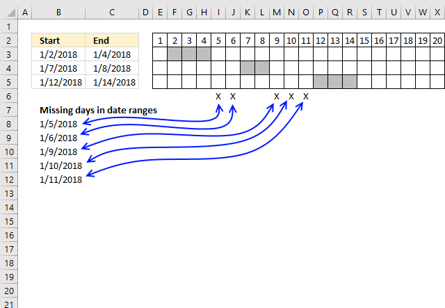
The array formula in cell B3 creates a list of dates based on the date ranges displayed in D3:E7, it […]

Extract duplicate records
This article describes how to filter duplicate rows with the use of a formula.  It is, in fact, an array […]

Filter duplicate records
This article demonstrates how to filter duplicate records using a simple formula and an Excel defined table.

Filter overlapping date ranges
This blog article describes how to extract coinciding date ranges using array formulas, the image above shows random date ranges […]

Filter shared records from two tables
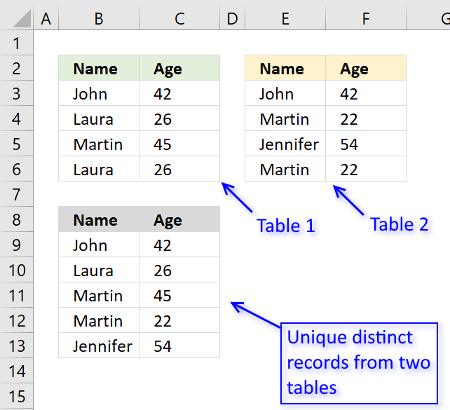
I will in this blog post demonstrate a formula that extracts common records (shared records) from two data sets in […]

Filter unique distinct records
Table of contents Filter unique distinct row records Filter unique distinct row records but not blanks Filter unique distinct row […]

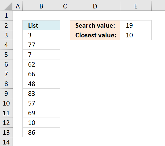
Find closest value
This article demonstrates formulas that extract the nearest number in a cell range to a condition. The image above shows […]

Highlight cells based on coordinates
The picture above shows Conditional Formatting highlighting cells in cell range F3:Y22 based on row and column values in column B […]

Highlight duplicate columns
This article describes how to highlight duplicate records arranged into a column each, if you are looking for records entered […]

Highlight duplicate records
This article shows you how to easily identify duplicate rows or records in a list. What’s on this webpage Highlight […]

Highlight unique distinct records
The image above demonstrates a Conditional Formatting formula that highlights unique distinct records. This means that the first instance of […]

How to compare two data sets
This article demonstrates how to quickly compare two data sets in Excel using a formula and Excel defined Tables. The […]

How to group items by quarter using formulas
This article demonstrates two formulas, the first formula counts items by quarter and the second formula extracts the corresponding items […]

Label groups of duplicate records
Michael asks: I need to identify the duplicates based on the Columns D:H and put in Column C a small […]

Lookup two index columns
Formula in B14: =INDEX(D3:D6, SUMPRODUCT(—(C10=B3:B6), —(C11=C3:C6), ROW(D3:D6)-MIN(ROW(D3:D6))+1)) Alternative array formula #1 in B15: =INDEX(D3:D6, MATCH(C10&»-«&C11, B3:B6&»-«&C3:C6, 0)) Alternative array formula […]

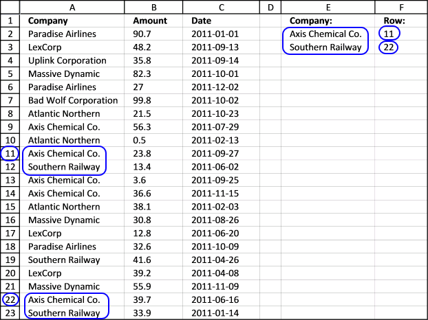
Lookup using multiple conditions
Debraj Roy asks:Hi Oscar, I failed to search for «Ask» Section.. so submitting my query here.. Apologize for hijacking someones […]

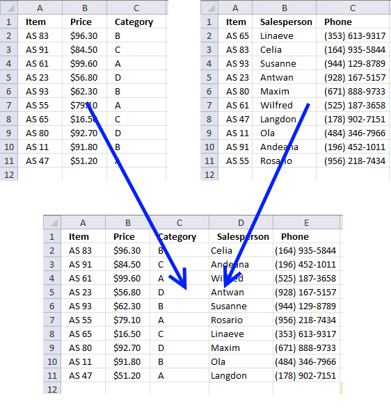
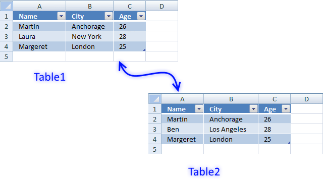
Merge tables based on a condition
This article demonstrates techniques on how to merge or combine two data sets using a condition. The top left data […]

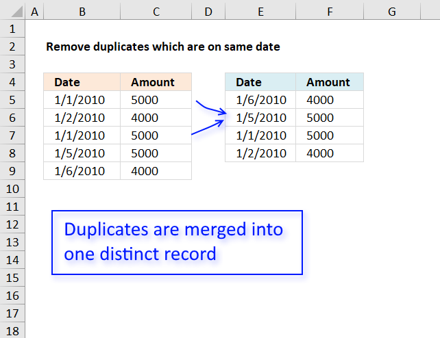
Remove duplicates based on date
Question: Column B has dates Column C as data B5 : 1/1/2010 : 5000 B6 : 2/1/2010 : 4000 B7 […]

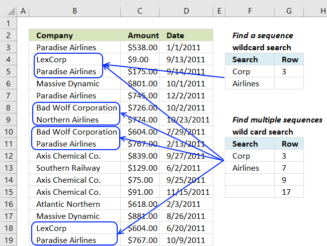
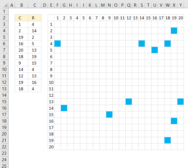
Search for a sequence of values
This article demonstrates array formulas that identify two search values in a row or in a sequence. The image above […]

SMALL function – multiple conditions
This article demonstrates how to sort numbers from small to large using a condition or criteria, I will show how […]

Working with three relational tables
I will in this article demonstrate four formulas that do lookups, extract unique distinct and duplicate values and sums numbers […]

Calculates the average of the absolute deviations of data points from their mean.

Calculates the average of numbers in a cell range.

Returns the average of a group of values. Text and boolean value FALSE evaluates to 0. TRUE to 1.

Returns the average of cell values that are valid for a given condition.

Returns the average of cell values that evaluates to TRUE for multiple criteria.

Calculates the beta distribution.

Calculates the inverse of the cumulative beta distribution.

Calculates the individual term binomial distribution probability.

Calculates the minimum value for which the binomial distribution is equal to or greater than a given threshold value.

Calculates the probability of the chi-squared distribution, cumulative distribution or probability density.

Calculates the right-tailed probability of the chi-squared distribution.

Calculates the inverse of the left-tailed probability of the chi-squared distribution.

Calculates the inverse of the right-tailed probability of the chi-squared distribution.

Calculates the test for independence, the value returned from the chi-squared statistical distribution and the correct degrees of freedom. Use this function to check if hypothesized results are valid.

Calculates the confidence interval for a population mean.

Calculates the confidence range for a population mean using a Student’s t distribution.

Calculates the correlation between two groups of numbers.

Counts all numerical values in an argument.

Counts the non-empty or non-blank cells in a cell range.

Counts empty or blank cells in a range.

Calculates the number of cells that is equal to a condition.

Calculates the number of cells across multiple ranges that equals all given conditions.

Calculates the covariance meaning the average of the products of deviations for each pair in two different datasets.

Calculates the sample covariance meaning the average of the products of deviations for each pair in two different datasets.

Calculates the exponential distribution representing an outcome in the form of probability.

Calculates the F probability for two tests.

Calculates the right-tailed F probability for two tests.

Calculates the two-tailed probability from an F-test

Calculates a value based on existing x and y values using linear regression.

Calculates how often values occur within a range of values and then returns a vertical array of numbers.

Calculates the GAMMA value.

Calculates the gamma often used in queuing analysis (probability statistics) that may have a skewed distribution.

Calculates the geometric mean.

Returns estimated exponential growth based on given data.

Returns a value representing the y-value where a line intersects the y-axis.

Calculates the k-th largest value from an array of numbers.

Returns an array of values representing the parameters of a straight line based on the «least squares» method.

Returns an array of values representing the parameters of an exponential curve that fits your data, based on the «least squares» method.

Calculates the lognormal distribution of argument x, based on a normally distributed ln(x) with the arguments of mean and standard_dev.

Calculate the largest number in a cell range.

Calculates the highest value based on a condition or criteria.

Calculates the median based on a group of numbers. The median is the middle number of a group of numbers.

Returns the smallest number in a cell range.

Returns the smallest number. Text values and blanks are ignored, boolean value TRUE evaluates to 1 and FALSE to 0 (zero).

Calculates the smallest value based on a given set of criteria.

Returns the most frequent number in a cell range. It will return multiple numbers if they are equally frequent.

Calculates the most frequent value in an array or range of data.

Calculates the normal distribution for a given mean and standard deviation.

Calculates the inverse of the normal cumulative distribution for a given mean and standard deviation.

Calculates the percent rank of a given number in a data set.

Calculates the percent rank of a given number compared to the whole data set.

Returns the number of permutations for a set of elements that can be selected from a larger number of elements.

Returns the number of permutations for a specific number of elements that can be selected from a larger group of elements.

Calculates a number of the density function for a standard normal distribution.

Calculates the probability that values in a range are between a given lower and upper limit.

Returns the quartile of a data set.

Returns the quartile of a data set, based on percentile values from 0..1, inclusive.

Returns the rank of a number out of a list of numbers.

Calculates the rank of a number in a list of numbers, based on its position if the list were sorted.

Calculates the skewness of a group of values.

Calculates the slope of the linear regression line through coordinates.

Returns the k-th smallest value from a group of numbers.

Calculates a normalized value from a distribution characterized by mean and standard_dev.

Returns standard deviation based on the entire population.

Returns standard deviation based on a sample of the entire population.

Estimates the standard deviation from a sample of values.

Returns the standard deviation based on the entire population, including text and logical values.

Calculates values along a linear trend.

Calculates the mean of the interior of a data set.

Returns the variance based on the entire population. The function ignores logical and text values.

The VAR.S function tries to estimate the variance based on a sample of the population. The function ignores logical and text values.

Excel has many functions where a user needs to specify a single or multiple criteria to get the result. For example, if you want to count cells based on multiple criteria, you can use the COUNTIF or COUNTIFS functions in Excel.

This tutorial covers various ways of using a single or multiple criteria in COUNTIF and COUNTIFS function in Excel.

While I will primarily be focussing on COUNTIF and COUNTIFS functions in this tutorial, all these examples can also be used in other Excel functions that take multiple criteria as inputs (such as SUMIF, SUMIFS, AVERAGEIF, and AVERAGEIFS).

An Introduction to Excel COUNTIF and COUNTIFS Functions

Let’s first get a grip on using COUNTIF and COUNTIFS functions in Excel.

Excel COUNTIF Function (takes Single Criteria)

Excel COUNTIF function is best suited for situations when you want to count cells based on a single criterion. If you want to count based on multiple criteria, use COUNTIFS function.

Syntax

=COUNTIF(range, criteria)

Input Arguments

• range –  the range of cells which you want to count.
• criteria – the criteria that must be evaluated against the range of cells for a cell to be counted.

Excel COUNTIFS Function (takes Multiple Criteria)

Excel COUNTIFS function is best suited for situations when you want to count cells based on multiple criteria.

Syntax

=COUNTIFS(criteria_range1, criteria1, [criteria_range2, criteria2]…)

Input Arguments

• criteria_range1 – The range of cells for which you want to evaluate against criteria1.
• criteria1 – the criteria which you want to evaluate for criteria_range1 to determine which cells to count.
• [criteria_range2] – The range of cells for which you want to evaluate against criteria2.
• [criteria2] – the criteria which you want to evaluate for criteria_range2 to determine which cells to count.

Now let’s have a look at some examples of using multiple criteria in COUNTIF functions in Excel.

Using NUMBER Criteria in Excel COUNTIF Functions

#1 Count Cells when Criteria is EQUAL to a Value

To get the count of cells where the criteria argument is equal to a specified value, you can either directly enter the criteria or use the cell reference that contains the criteria.

Below is an example where we count the cells that contain the number 9 (which means that the criteria argument is equal to 9). Here is the formula:

=COUNTIF($B$2:$B$11,D3)

In the above example (in the pic), the criteria is in cell D3. You can also enter the criteria directly into the formula. For example, you can also use:

=COUNTIF($B$2:$B$11,9)

#2 Count Cells when Criteria is GREATER THAN a Value

To get the count of cells with a value greater than a specified value, we use the greater than operator (“>”). We could either use it directly in the formula or use a cell reference that has the criteria.

Whenever we use an operator in criteria in Excel, we need to put it within double quotes. For example, if the criteria is greater than 10, then we need to enter “>10” as the criteria (see pic below):

Here is the formula:

=COUNTIF($B$2:$B$11,”>10″)

You can also have the criteria in a cell and use the cell reference as the criteria. In this case, you need NOT put the criteria in double quotes:

=COUNTIF($B$2:$B$11,D3)

There could also be a case when you want the criteria to be in a cell, but don’t want it with the operator. For example, you may want the cell D3 to have the number 10 and not >10.

In that case, you need to create a criteria argument which is a combination of operator and cell reference (see pic below):

=COUNTIF($B$2:$B$11,”>”&D3)

NOTE: When you combine an operator and a cell reference, the operator is always in double quotes. The operator and cell reference are joined by an ampersand (&).

#3 Count Cells when Criteria is LESS THAN a Value

To get the count of cells with a value less than a specified value, we use the less than operator (“<“). We could either use it directly in the formula or use a cell reference that has the criteria.

Whenever we use an operator in criteria in Excel, we need to put it within double quotes. For example, if the criterion is that the number should be less than 5, then we need to enter “<5” as the criteria (see pic below):

=COUNTIF($B$2:$B$11,”<5″)

You can also have the criteria in a cell and use the cell reference as the criteria. In this case, you need NOT put the criteria in double quotes (see pic below):

=COUNTIF($B$2:$B$11,D3)

Also, there could be a case when you want the criteria to be in a cell, but don’t want it with the operator. For example, you may want the cell D3 to have the number 5 and not <5.

In that case, you need to create a criteria argument which is a combination of operator and cell reference:

=COUNTIF($B$2:$B$11,”<“&D3)

NOTE: When you combine an operator and a cell reference, the operator is always in double quotes. The operator and cell reference are joined by an ampersand (&).

#4 Count Cells with Multiple Criteria – Between Two Values

To get a count of values between two values, we need to use multiple criteria in the COUNTIF function.

Here are two methods of doing this:

METHOD 1: Using COUNTIFS function

COUNTIFS function can handle multiple criteria as arguments and counts the cells only when all the criteria are TRUE. To count cells with values between two specified values (say 5 and 10), we can use the following COUNTIFS function:

=COUNTIFS($B$2:$B$11,”>5″,$B$2:$B$11,”<10″)

NOTE: The above formula does not count cells that contain 5 or 10. If you want to include these cells, use greater than equal to (>=) and less than equal to (<=) operators. Here is the formula:

=COUNTIFS($B$2:$B$11,”>=5″,$B$2:$B$11,”<=10″) 

You can also have these criteria in cells and use the cell reference as the criteria. In this case, you need NOT put the criteria in double quotes (see pic below):

You can also use a combination of cells references and operators (where the operator is entered directly in the formula). When you combine an operator and a cell reference, the operator is always in double quotes. The operator and cell reference are joined by an ampersand (&).

METHOD 2: Using two COUNTIF functions

If you have multiple criteria, you can either use COUNTIFS or create a combination of COUNTIF functions. The formula below would also do the same thing:

=COUNTIF($B$2:$B$11,”>5″)-COUNTIF($B$2:$B$11,”>10″)

In the above formula, we first find the number of cells that have a value greater than 5 and we subtract the count of cells with a value greater than 10. This would give us the result as 5 (which is the number of cells that have values more than 5 and less than equal to 10).

If you want the formula to include both 5 and 10, use the following formula instead:

=COUNTIF($B$2:$B$11,”>=5″)-COUNTIF($B$2:$B$11,”>10″)

If you want the formula to exclude both ‘5’ and ’10’ from the counting, use the following formula:

=COUNTIF($B$2:$B$11,”>=5″)-COUNTIF($B$2:$B$11,”>10″)-COUNTIF($B$2:$B$11,10)

You can have these criteria in cells and use the cells references, or you can use a combination of operators and cells references.

Using TEXT Criteria in Excel Functions

#1 Count Cells when Criteria is EQUAL to a Specified text

To count cells that contain an exact match of the specified text, we can simply use that text as the criteria. For example, in the dataset (shown below in the pic), if I want to count all the cells with the name Joe in it, I can use the below formula:

=COUNTIF($B$2:$B$11,”Joe”)

Since this is a text string, I need to put the text criteria in double quotes.

You can also have the criteria in a cell and then use that cell reference (as shown below):

=COUNTIF($B$2:$B$11,E3)

NOTE: You can get wrong results if there are leading/trailing spaces in the criteria or criteria range. Make sure you clean the data before using these formulas.

#2 Count Cells when Criteria is NOT EQUAL to a Specified text

Similar to what we saw in the above example, you can also count cells that do not contain a specified text. To do this, we need to use the not equal to operator (<>).

Suppose you want to count all the cells that do not contain the name JOE, here is the formula that will do it:

=COUNTIF($B$2:$B$11,”<>Joe”)

You can also have the criteria in a cell and use the cell reference as the criteria. In this case, you need NOT put the criteria in double quotes (see pic below):

=COUNTIF($B$2:$B$11,E3)

There could also be a case when you want the criteria to be in a cell but don’t want it with the operator. For example, you may want the cell D3 to have the name Joe and not <>Joe.

In that case, you need to create a criteria argument which is a combination of operator and cell reference (see pic below):

=COUNTIF($B$2:$B$11,”<>”&E3)

When you combine an operator and a cell reference, the operator is always in double quotes. The operator and cell reference are joined by an ampersand (&).

Using DATE Criteria in Excel COUNTIF and COUNTIFS Functions

Excel store date and time as numbers. So we can use it the same way we use numbers.

#1 Count Cells when Criteria is EQUAL to a Specified Date

To get the count of cells that contain the specified date, we would use the equal to operator (=) along with the date.

To use the date, I recommend using the DATE function, as it gets rid of any possibility of error in the date value. So, for example, if I want to use the date September 1, 2015, I can use the DATE function as shown below:

=DATE(2015,9,1)

This formula would return the same date despite regional differences. For example, 01-09-2015 would be September 1, 2015 according to the  US date syntax and January 09, 2015 according to the UK date syntax. However, this formula would always return September 1, 2105.

Here is the formula to count the number of cells that contain the date 02-09-2015:

=COUNTIF($A$2:$A$11,DATE(2015,9,2))

#2 Count Cells when Criteria is BEFORE or AFTER to a Specified Date

To count cells that contain date before or after a specified date, we can use the less than/greater than operators.

For example, if I want to count all the cells that contain a date that is after September 02, 2015, I can use the formula:

=COUNTIF($A$2:$A$11,”>”&DATE(2015,9,2))

Similarly, you can also count the number of cells before a specified date. If you want to include a date in the counting, use and ‘equal to’ operator along with ‘greater than/less than’ operator.

You can also use a cell reference that contains a date. In this case, you need to combine the operator (within double quotes) with the date using an ampersand (&).

See example below:

=COUNTIF($A$2:$A$11,”>”&F3)

#3 Count Cells with Multiple Criteria – Between Two Dates

To get a count of values between two values, we need to use multiple criteria in the COUNTIF function.

We can do this using two methods – One single COUNTIFS function or two COUNTIF functions.

METHOD 1: Using COUNTIFS function

COUNTIFS function can take multiple criteria as the arguments and counts the cells only when all the criteria are TRUE. To count cells with values between two specified dates (say September 2 and September 7), we can use the following COUNTIFS function:

=COUNTIFS($A$2:$A$11,”>”&DATE(2015,9,2),$A$2:$A$11,”<“&DATE(2015,9,7))

The above formula does not count cells that contain the specified dates. If you want to include these dates as well, use greater than equal to (>=) and less than equal to (<=) operators. Here is the formula:

=COUNTIFS($A$2:$A$11,”>=”&DATE(2015,9,2),$A$2:$A$11,”<=”&DATE(2015,9,7))

You can also have the dates in a cell and use the cell reference as the criteria. In this case, you can not have the operator with the date in the cells. You need to manually add operators in the formula (in double quotes) and add cell reference using an ampersand (&). See the pic below:

=COUNTIFS($A$2:$A$11,”>”&F3,$A$2:$A$11,”<“&G3)

METHOD 2: Using COUNTIF functions

If you have multiple criteria, you can either use one COUNTIFS function or create a combination of two COUNTIF functions. The formula below would also do the trick:

=COUNTIF($A$2:$A$11,”>”&DATE(2015,9,2))-COUNTIF($A$2:$A$11,”>”&DATE(2015,9,7))

In the above formula, we first find the number of cells that have a date after September 2 and we subtract the count of cells with dates after September 7. This would give us the result as 7 (which is the number of cells that have dates after September 2 and on or before September 7).

If you don’t want the formula to count both September 2 and September 7, use the following formula instead:

=COUNTIF($A$2:$A$11,”>=”&DATE(2015,9,2))-COUNTIF($A$2:$A$11,”>”&DATE(2015,9,7))

If you want to exclude both the dates from counting, use the following formula:

=COUNTIF($A$2:$A$11,”>”&DATE(2015,9,2))-COUNTIF($A$2:$A$11,”>”&DATE(2015,9,7)-COUNTIF($A$2:$A$11,DATE(2015,9,7)))

Also, you can have the criteria dates in cells and use the cells references (along with operators in double quotes joined using ampersand).

Using WILDCARD CHARACTERS in Criteria in COUNTIF & COUNTIFS Functions

There are three wildcard characters in Excel:

1. * (asterisk) – It represents any number of characters. For example, ex* could mean excel, excels, example, expert, etc.
2. ? (question mark) – It represents one single character. For example, Tr?mp could mean Trump or Tramp.
3. ~ (tilde) – It is used to identify a wildcard character (~, *, ?) in the text.

You can use COUNTIF function with wildcard characters to count cells when other inbuilt count function fails. For example, suppose you have a data set as shown below:

Now let’s take various examples:

#1 Count Cells that contain Text

To count cells with text in it, we can use the wildcard character * (asterisk). Since asterisk represents any number of characters, it would count all cells that have any text in it. Here is the formula:

=COUNTIFS($C$2:$C$11,”*”)

Note: The formula above ignores cells that contain numbers, blank cells, and logical values, but would count the cells contain an apostrophe (and hence appear blank) or cells that contain empty string (=””) which may have been returned as a part of a formula.

Here is a detailed tutorial on handling cases where there is an empty string or apostrophe.

Here is a detailed tutorial on handling cases where there are empty strings or apostrophes.

Below is a video that explains different scenarios of counting cells with text in it.

#2 Count Non-blank Cells

If you are thinking of using COUNTA function, think again.

Try it and it might fail you. COUNTA will also count a cell that contains an empty string (often returned by formulas as =”” or when people enter only an apostrophe in a cell). Cells that contain empty strings look blank but are not, and thus counted by the COUNTA function.

COUNTA will also count a cell that contains an empty string (often returned by formulas as =”” or when people enter only an apostrophe in a cell). Cells that contain empty strings look blank but are not, and thus counted by the COUNTA function.

So if you use the formula =COUNTA(A1:A11), it returns 11, while it should return 10.

Here is the fix:

=COUNTIF($A$1:$A$11,”?*”)+COUNT($A$1:$A$11)+SUMPRODUCT(–ISLOGICAL($A$1:$A$11))

Let’s understand this formula by breaking it down:

#3 Count Cells that contain specific text

Let’s say we want to count all the cells where the sales rep name begins with J. This can easily be achieved by using a wildcard character in COUNTIF function. Here is the formula:

=COUNTIFS($C$2:$C$11,”J*”) 

The criteria J* specifies that the text in a cell should begin with J and can contain any number of characters.

If you want to count cells that contain the alphabet anywhere in the text, flank it with an asterisk on both sides. For example, if you want to count cells that contain the alphabet “a” in it, use *a* as the criteria.

This article is unusually long compared to my other articles. Hope you have enjoyed it. Let me know your thoughts by leaving a comment.

You May Also Find the following Excel tutorials useful:

• Count the number of words in Excel.
• Count Cells Based on Background Color in Excel.
• How to Sum a Column in Excel (5 Really Easy Ways)