
Excel for Microsoft 365 Excel for Microsoft 365 for Mac Excel for the web Excel 2021 Excel 2021 for Mac Excel 2019 Excel 2019 for Mac Excel 2016 Excel 2016 for Mac Excel 2013 Excel Web App Excel 2010 More…Less
The COUNTIFS function applies criteria to cells across multiple ranges and counts the number of times all criteria are met.

This video is part of a training course called Advanced IF functions.
Syntax
COUNTIFS(criteria_range1, criteria1, [criteria_range2, criteria2]…)
The COUNTIFS function syntax has the following arguments:
-
criteria_range1 Required. The first range in which to evaluate the associated criteria.
-
criteria1 Required. The criteria in the form of a number, expression, cell reference, or text that define which cells will be counted. For example, criteria can be expressed as 32, «>32», B4, «apples», or «32».
-
criteria_range2, criteria2, … Optional. Additional ranges and their associated criteria. Up to 127 range/criteria pairs are allowed.
Important: Each additional range must have the same number of rows and columns as the criteria_range1 argument. The ranges do not have to be adjacent to each other.
Remarks
-
Each range’s criteria is applied one cell at a time. If all of the first cells meet their associated criteria, the count increases by 1. If all of the second cells meet their associated criteria, the count increases by 1 again, and so on until all of the cells are evaluated.
-
If the criteria argument is a reference to an empty cell, the COUNTIFS function treats the empty cell as a 0 value.
-
You can use the wildcard characters— the question mark (?) and asterisk (*) — in criteria. A question mark matches any single character, and an asterisk matches any sequence of characters. If you want to find an actual question mark or asterisk, type a tilde (~) before the character.
Example 1
Copy the example data in the following tables, and paste it in cell A1 of a new Excel worksheet. For formulas to show results, select them, press F2, and then press Enter. If you need to, you can adjust the column widths to see all the data.
|
Salesperson |
Exceeded Q1 quota |
Exceeded Q2 quota |
Exceeded Q3 quota |
|---|---|---|---|
|
Davidoski |
Yes |
No |
No |
|
Burke |
Yes |
Yes |
No |
|
Sundaram |
Yes |
Yes |
Yes |
|
Levitan |
No |
Yes |
Yes |
|
Formula |
Description |
Result |
|
|
=COUNTIFS(B2:D2,»=Yes») |
Counts how many times Davidoski exceeded a sales quota for periods Q1, Q2, and Q3 (only in Q1). |
1 |
|
|
=COUNTIFS(B2:B5,»=Yes»,C2:C5,»=Yes») |
Counts how many salespeople exceeded both their Q1 and Q2 quotas (Burke and Sundaram). |
2 |
|
|
=COUNTIFS(B5:D5,»=Yes»,B3:D3,»=Yes») |
Counts how many times Levitan and Burke exceeded the same quota for periods Q1, Q2, and Q3 (only in Q2). |
1 |
Example 2
|
Data |
||
|---|---|---|
|
1 |
5/1/2011 |
|
|
2 |
5/2/2011 |
|
|
3 |
5/3/2011 |
|
|
4 |
5/4/2011 |
|
|
5 |
5/5/2011 |
|
|
6 |
5/6/2011 |
|
|
Formula |
Description |
Result |
|
=COUNTIFS(A2:A7,»<6″,A2:A7,»>1″) |
Counts how many numbers between 1 and 6 (not including 1 and 6) are contained in cells A2 through A7. |
4 |
|
=COUNTIFS(A2:A7, «<5″,B2:B7,»<5/3/2011») |
Counts how many rows have numbers that are less than 5 in cells A2 through A7, and also have dates that are are earlier than 5/3/2011 in cells B2 through B7. |
2 |
|
=COUNTIFS(A2:A7, «<» & A6,B2:B7,»<» & B4) |
Same description as the previous example, but using cell references instead of constants in the criteria. |
2 |
Need more help?
You can always ask an expert in the Excel Tech Community or get support in the Answers community.
See Also
To count cells that aren’t blank, use the COUNTA function
To count cells using a single criteria, use the COUNTIF function
The SUMIF function adds only the values that meet a single criteria
The SUMIFS function adds only the values that meet multiple criteria
IFS function (Microsoft 365, Excel 2016 and later)
Overview of formulas in Excel
How to avoid broken formulas
Detect errors in formulas
Statistical functions
Excel functions (alphabetical)
Excel functions (by Category)
Need more help?
Want more options?
Explore subscription benefits, browse training courses, learn how to secure your device, and more.
Communities help you ask and answer questions, give feedback, and hear from experts with rich knowledge.
Excel has many functions where a user needs to specify a single or multiple criteria to get the result. For example, if you want to count cells based on multiple criteria, you can use the COUNTIF or COUNTIFS functions in Excel.
This tutorial covers various ways of using a single or multiple criteria in COUNTIF and COUNTIFS function in Excel.
While I will primarily be focussing on COUNTIF and COUNTIFS functions in this tutorial, all these examples can also be used in other Excel functions that take multiple criteria as inputs (such as SUMIF, SUMIFS, AVERAGEIF, and AVERAGEIFS).
An Introduction to Excel COUNTIF and COUNTIFS Functions
Let’s first get a grip on using COUNTIF and COUNTIFS functions in Excel.
Excel COUNTIF Function (takes Single Criteria)
Excel COUNTIF function is best suited for situations when you want to count cells based on a single criterion. If you want to count based on multiple criteria, use COUNTIFS function.
Syntax
=COUNTIF(range, criteria)
Input Arguments
- range – the range of cells which you want to count.
- criteria – the criteria that must be evaluated against the range of cells for a cell to be counted.
Excel COUNTIFS Function (takes Multiple Criteria)
Excel COUNTIFS function is best suited for situations when you want to count cells based on multiple criteria.
Syntax
=COUNTIFS(criteria_range1, criteria1, [criteria_range2, criteria2]…)
Input Arguments
- criteria_range1 – The range of cells for which you want to evaluate against criteria1.
- criteria1 – the criteria which you want to evaluate for criteria_range1 to determine which cells to count.
- [criteria_range2] – The range of cells for which you want to evaluate against criteria2.
- [criteria2] – the criteria which you want to evaluate for criteria_range2 to determine which cells to count.
Now let’s have a look at some examples of using multiple criteria in COUNTIF functions in Excel.
Using NUMBER Criteria in Excel COUNTIF Functions
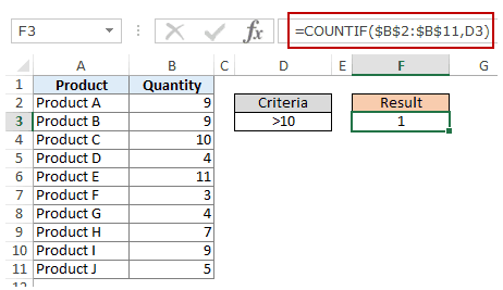
#1 Count Cells when Criteria is EQUAL to a Value
To get the count of cells where the criteria argument is equal to a specified value, you can either directly enter the criteria or use the cell reference that contains the criteria.
Below is an example where we count the cells that contain the number 9 (which means that the criteria argument is equal to 9). Here is the formula:
=COUNTIF($B$2:$B$11,D3)

In the above example (in the pic), the criteria is in cell D3. You can also enter the criteria directly into the formula. For example, you can also use:
=COUNTIF($B$2:$B$11,9)
#2 Count Cells when Criteria is GREATER THAN a Value
To get the count of cells with a value greater than a specified value, we use the greater than operator (“>”). We could either use it directly in the formula or use a cell reference that has the criteria.
Whenever we use an operator in criteria in Excel, we need to put it within double quotes. For example, if the criteria is greater than 10, then we need to enter “>10” as the criteria (see pic below):
Here is the formula:
=COUNTIF($B$2:$B$11,”>10″)

You can also have the criteria in a cell and use the cell reference as the criteria. In this case, you need NOT put the criteria in double quotes:
=COUNTIF($B$2:$B$11,D3)
There could also be a case when you want the criteria to be in a cell, but don’t want it with the operator. For example, you may want the cell D3 to have the number 10 and not >10.
In that case, you need to create a criteria argument which is a combination of operator and cell reference (see pic below):
=COUNTIF($B$2:$B$11,”>”&D3)
 NOTE: When you combine an operator and a cell reference, the operator is always in double quotes. The operator and cell reference are joined by an ampersand (&).
#3 Count Cells when Criteria is LESS THAN a Value
To get the count of cells with a value less than a specified value, we use the less than operator (“<“). We could either use it directly in the formula or use a cell reference that has the criteria.
Whenever we use an operator in criteria in Excel, we need to put it within double quotes. For example, if the criterion is that the number should be less than 5, then we need to enter “<5” as the criteria (see pic below):
=COUNTIF($B$2:$B$11,”<5″)

You can also have the criteria in a cell and use the cell reference as the criteria. In this case, you need NOT put the criteria in double quotes (see pic below):
=COUNTIF($B$2:$B$11,D3)

Also, there could be a case when you want the criteria to be in a cell, but don’t want it with the operator. For example, you may want the cell D3 to have the number 5 and not <5.
In that case, you need to create a criteria argument which is a combination of operator and cell reference:
=COUNTIF($B$2:$B$11,”<“&D3)

NOTE: When you combine an operator and a cell reference, the operator is always in double quotes. The operator and cell reference are joined by an ampersand (&).
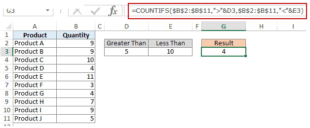
#4 Count Cells with Multiple Criteria – Between Two Values
To get a count of values between two values, we need to use multiple criteria in the COUNTIF function.
Here are two methods of doing this:
METHOD 1: Using COUNTIFS function
COUNTIFS function can handle multiple criteria as arguments and counts the cells only when all the criteria are TRUE. To count cells with values between two specified values (say 5 and 10), we can use the following COUNTIFS function:
=COUNTIFS($B$2:$B$11,”>5″,$B$2:$B$11,”<10″)

NOTE: The above formula does not count cells that contain 5 or 10. If you want to include these cells, use greater than equal to (>=) and less than equal to (<=) operators. Here is the formula:
=COUNTIFS($B$2:$B$11,”>=5″,$B$2:$B$11,”<=10″)
You can also have these criteria in cells and use the cell reference as the criteria. In this case, you need NOT put the criteria in double quotes (see pic below):

You can also use a combination of cells references and operators (where the operator is entered directly in the formula). When you combine an operator and a cell reference, the operator is always in double quotes. The operator and cell reference are joined by an ampersand (&).
METHOD 2: Using two COUNTIF functions
If you have multiple criteria, you can either use COUNTIFS or create a combination of COUNTIF functions. The formula below would also do the same thing:
=COUNTIF($B$2:$B$11,”>5″)-COUNTIF($B$2:$B$11,”>10″)
In the above formula, we first find the number of cells that have a value greater than 5 and we subtract the count of cells with a value greater than 10. This would give us the result as 5 (which is the number of cells that have values more than 5 and less than equal to 10).
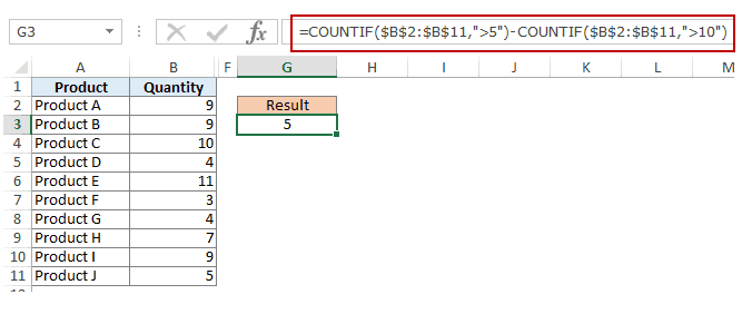
If you want the formula to include both 5 and 10, use the following formula instead:
=COUNTIF($B$2:$B$11,”>=5″)-COUNTIF($B$2:$B$11,”>10″)
If you want the formula to exclude both ‘5’ and ’10’ from the counting, use the following formula:
=COUNTIF($B$2:$B$11,”>=5″)-COUNTIF($B$2:$B$11,”>10″)-COUNTIF($B$2:$B$11,10)
You can have these criteria in cells and use the cells references, or you can use a combination of operators and cells references.
Using TEXT Criteria in Excel Functions
#1 Count Cells when Criteria is EQUAL to a Specified text
To count cells that contain an exact match of the specified text, we can simply use that text as the criteria. For example, in the dataset (shown below in the pic), if I want to count all the cells with the name Joe in it, I can use the below formula:
=COUNTIF($B$2:$B$11,”Joe”)
Since this is a text string, I need to put the text criteria in double quotes.
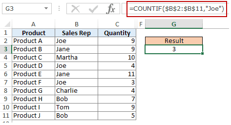
You can also have the criteria in a cell and then use that cell reference (as shown below):
=COUNTIF($B$2:$B$11,E3)

NOTE: You can get wrong results if there are leading/trailing spaces in the criteria or criteria range. Make sure you clean the data before using these formulas.
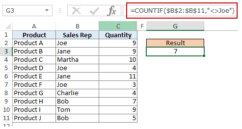
#2 Count Cells when Criteria is NOT EQUAL to a Specified text
Similar to what we saw in the above example, you can also count cells that do not contain a specified text. To do this, we need to use the not equal to operator (<>).
Suppose you want to count all the cells that do not contain the name JOE, here is the formula that will do it:
=COUNTIF($B$2:$B$11,”<>Joe”)
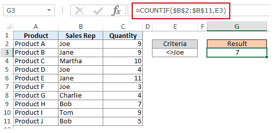
You can also have the criteria in a cell and use the cell reference as the criteria. In this case, you need NOT put the criteria in double quotes (see pic below):
=COUNTIF($B$2:$B$11,E3)
There could also be a case when you want the criteria to be in a cell but don’t want it with the operator. For example, you may want the cell D3 to have the name Joe and not <>Joe.
In that case, you need to create a criteria argument which is a combination of operator and cell reference (see pic below):
=COUNTIF($B$2:$B$11,”<>”&E3)
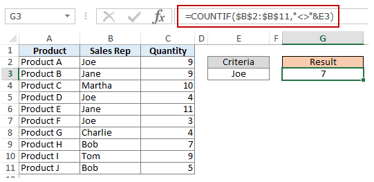
When you combine an operator and a cell reference, the operator is always in double quotes. The operator and cell reference are joined by an ampersand (&).
Using DATE Criteria in Excel COUNTIF and COUNTIFS Functions
Excel store date and time as numbers. So we can use it the same way we use numbers.
#1 Count Cells when Criteria is EQUAL to a Specified Date
To get the count of cells that contain the specified date, we would use the equal to operator (=) along with the date.
To use the date, I recommend using the DATE function, as it gets rid of any possibility of error in the date value. So, for example, if I want to use the date September 1, 2015, I can use the DATE function as shown below:
=DATE(2015,9,1)
This formula would return the same date despite regional differences. For example, 01-09-2015 would be September 1, 2015 according to the US date syntax and January 09, 2015 according to the UK date syntax. However, this formula would always return September 1, 2105.
Here is the formula to count the number of cells that contain the date 02-09-2015:
=COUNTIF($A$2:$A$11,DATE(2015,9,2))

#2 Count Cells when Criteria is BEFORE or AFTER to a Specified Date
To count cells that contain date before or after a specified date, we can use the less than/greater than operators.
For example, if I want to count all the cells that contain a date that is after September 02, 2015, I can use the formula:
=COUNTIF($A$2:$A$11,”>”&DATE(2015,9,2))

Similarly, you can also count the number of cells before a specified date. If you want to include a date in the counting, use and ‘equal to’ operator along with ‘greater than/less than’ operator.
You can also use a cell reference that contains a date. In this case, you need to combine the operator (within double quotes) with the date using an ampersand (&).
See example below:
=COUNTIF($A$2:$A$11,”>”&F3)

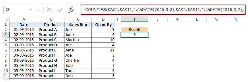
#3 Count Cells with Multiple Criteria – Between Two Dates
To get a count of values between two values, we need to use multiple criteria in the COUNTIF function.
We can do this using two methods – One single COUNTIFS function or two COUNTIF functions.
METHOD 1: Using COUNTIFS function
COUNTIFS function can take multiple criteria as the arguments and counts the cells only when all the criteria are TRUE. To count cells with values between two specified dates (say September 2 and September 7), we can use the following COUNTIFS function:
=COUNTIFS($A$2:$A$11,”>”&DATE(2015,9,2),$A$2:$A$11,”<“&DATE(2015,9,7))
The above formula does not count cells that contain the specified dates. If you want to include these dates as well, use greater than equal to (>=) and less than equal to (<=) operators. Here is the formula:
=COUNTIFS($A$2:$A$11,”>=”&DATE(2015,9,2),$A$2:$A$11,”<=”&DATE(2015,9,7))
You can also have the dates in a cell and use the cell reference as the criteria. In this case, you can not have the operator with the date in the cells. You need to manually add operators in the formula (in double quotes) and add cell reference using an ampersand (&). See the pic below:
=COUNTIFS($A$2:$A$11,”>”&F3,$A$2:$A$11,”<“&G3)

METHOD 2: Using COUNTIF functions
If you have multiple criteria, you can either use one COUNTIFS function or create a combination of two COUNTIF functions. The formula below would also do the trick:
=COUNTIF($A$2:$A$11,”>”&DATE(2015,9,2))-COUNTIF($A$2:$A$11,”>”&DATE(2015,9,7))
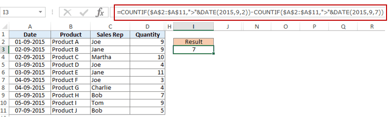
In the above formula, we first find the number of cells that have a date after September 2 and we subtract the count of cells with dates after September 7. This would give us the result as 7 (which is the number of cells that have dates after September 2 and on or before September 7).
If you don’t want the formula to count both September 2 and September 7, use the following formula instead:
=COUNTIF($A$2:$A$11,”>=”&DATE(2015,9,2))-COUNTIF($A$2:$A$11,”>”&DATE(2015,9,7))

If you want to exclude both the dates from counting, use the following formula:
=COUNTIF($A$2:$A$11,”>”&DATE(2015,9,2))-COUNTIF($A$2:$A$11,”>”&DATE(2015,9,7)-COUNTIF($A$2:$A$11,DATE(2015,9,7)))
Also, you can have the criteria dates in cells and use the cells references (along with operators in double quotes joined using ampersand).
Using WILDCARD CHARACTERS in Criteria in COUNTIF & COUNTIFS Functions
There are three wildcard characters in Excel:
- * (asterisk) – It represents any number of characters. For example, ex* could mean excel, excels, example, expert, etc.
- ? (question mark) – It represents one single character. For example, Tr?mp could mean Trump or Tramp.
- ~ (tilde) – It is used to identify a wildcard character (~, *, ?) in the text.
You can use COUNTIF function with wildcard characters to count cells when other inbuilt count function fails. For example, suppose you have a data set as shown below:
Now let’s take various examples:
#1 Count Cells that contain Text
To count cells with text in it, we can use the wildcard character * (asterisk). Since asterisk represents any number of characters, it would count all cells that have any text in it. Here is the formula:
=COUNTIFS($C$2:$C$11,”*”)
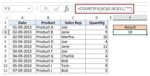
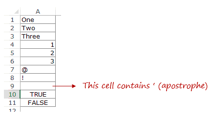
Note: The formula above ignores cells that contain numbers, blank cells, and logical values, but would count the cells contain an apostrophe (and hence appear blank) or cells that contain empty string (=””) which may have been returned as a part of a formula.
Here is a detailed tutorial on handling cases where there is an empty string or apostrophe.
Here is a detailed tutorial on handling cases where there are empty strings or apostrophes.
Below is a video that explains different scenarios of counting cells with text in it.
#2 Count Non-blank Cells
If you are thinking of using COUNTA function, think again.
Try it and it might fail you. COUNTA will also count a cell that contains an empty string (often returned by formulas as =”” or when people enter only an apostrophe in a cell). Cells that contain empty strings look blank but are not, and thus counted by the COUNTA function.
COUNTA will also count a cell that contains an empty string (often returned by formulas as =”” or when people enter only an apostrophe in a cell). Cells that contain empty strings look blank but are not, and thus counted by the COUNTA function.
So if you use the formula =COUNTA(A1:A11), it returns 11, while it should return 10.
Here is the fix:
=COUNTIF($A$1:$A$11,”?*”)+COUNT($A$1:$A$11)+SUMPRODUCT(–ISLOGICAL($A$1:$A$11))
Let’s understand this formula by breaking it down:
#3 Count Cells that contain specific text
Let’s say we want to count all the cells where the sales rep name begins with J. This can easily be achieved by using a wildcard character in COUNTIF function. Here is the formula:
=COUNTIFS($C$2:$C$11,”J*”)

The criteria J* specifies that the text in a cell should begin with J and can contain any number of characters.
If you want to count cells that contain the alphabet anywhere in the text, flank it with an asterisk on both sides. For example, if you want to count cells that contain the alphabet “a” in it, use *a* as the criteria.
This article is unusually long compared to my other articles. Hope you have enjoyed it. Let me know your thoughts by leaving a comment.
You May Also Find the following Excel tutorials useful:
- Count the number of words in Excel.
- Count Cells Based on Background Color in Excel.
- How to Sum a Column in Excel (5 Really Easy Ways)
The COUNTIFS function counts cells in a range that meet one or more conditions, referred to as criteria. To apply conditions, the COUNTIFS function supports logical operators (>,<,<>,=) and wildcards (*,?) for partial matching. The COUNTIFS function is a common, widely used function in Excel, and can be used to count cells that contain dates, numbers, and text.
Syntax
The syntax for the COUNTIFS function depends on the criteria being evaluated. Each separate condition will require a range and a criteria. The generic syntax looks like this:
=COUNTIFS(range1,criteria1) // 1 condition
=COUNTIFS(range1,criteria1,range2,criteria2) // 2 conditions
The first two arguments, range1 and criteria1 are required. Range1 is the range to which criteria1 should be applied. Range2 is the range to which criteria2 should be applied. Additional conditions are applied by providing more range and criteria arguments: the third condition is defined by range3 and criteria3, the fourth condition is defined by range4 and criteria4, and so on. When using COUNTIFS, keep the following in mind:
- To be included in the final result, all conditions must be TRUE.
- All ranges must be the same size or COUNTIFS will return a #VALUE! error.
- Criteria should include logical operators (>,<,<>,<=,>=) as needed.
- Each new condition requires a separate range and criteria.
Criteria
The COUNTIFS function supports logical operators (>,<,<>,=) and wildcards (*,?) for partial matching. Because COUNTIFS is in a group of eight functions that split logical criteria into two parts, the syntax is a bit tricky. Each condition requires a separate range and criteria, and operators need to be enclosed in double quotes («»). The table below shows some common examples:
| Target | Criteria |
|---|---|
| Cells greater than 75 | «>75» |
| Cells equal to 100 | 100 or «100» |
| Cells less than or equal to 100 | «<=100» |
| Cells equal to «Red» | «red» |
| Cells not equal to «Red» | «<>red» |
| Cells that are blank «» | «» |
| Cells that are not blank | «<>» |
| Cells that begin with «X» | «x*» |
| Cells less than A1 | «<«&A1 |
| Cells less than today | «<«&TODAY() |
Notice the last two examples use concatenation with the ampersand (&) character. When a criteria argument includes a value from another cell, or the result of a formula, logical operators like «<» must be joined with concatenation. This is because Excel needs to evaluate cell references and formulas first to get a value before that value can be joined to an operator.
Basic example
With the example shown, COUNTIFS can be used to count records using 2 criteria as follows:
=COUNTIFS(C5:C14,"red",D5:D14,"tx") // red and TX
=COUNTIFS(C5:C14,"red",F5:F14,">20") // red and >20
Notice the COUNTIFS function is not case-sensitive.
Double quotes («») in criteria
In general, text values need to be enclosed in double quotes, and numbers do not. However, when a logical operator is included with a number, the number and operator must be enclosed in quotes as shown below:
=COUNTIFS(A1:A10,100) // count equal to 100
=COUNTIFS(A1:A10,">50") // count greater than 50
=COUNTIFS(A1:A10,"jim") // count equal to "jim"
Note: showing one condition only for simplicity. Additional conditions must follow the same rules.
Value from another cell
When using a value from another cell in a condition, the cell reference must be concatenated to an operator when used. In the example below, COUNTIFS will count the values in A1:A10 that are less than the value in cell B1. Notice the less than operator (which is text) is enclosed in quotes, but the cell reference is not:
=COUNTIFS(A1:A10,"<"&B1) // count cells less than B1
Note: COUNTIFS is one of several functions that split conditions into two parts: range + criteria. This causes some inconsistencies with respect to other formulas and functions.
Not equal to
To construct «not equal to» criteria, use the «<>» operator surrounded by double quotes («»). For example, the formula below will count cells not equal to «red» in the range A1:A10:
=COUNTIFS(A1:A10,"<>red") // not "red"
Blank cells
COUNTIFS can count cells that are blank or not blank. The formulas below count blank and not blank cells in the range A1:A10:
=COUNTIFS(A1:A10,"<>") // not blank
=COUNTIFS(A1:A10,"") // blank
Dates
The easiest way to use COUNTIFS with dates is to refer to a valid date in another cell with a cell reference. For example, to count cells in A1:A10 that contain a date greater than a date in B1, you can use a formula like this:
=COUNTIFS(A1:A10, ">"&B1) // count dates greater than A1
Notice we concatenate the «>» operator to the date in B1, but and are no quotes around the cell reference.
The safest way to hardcode a date into COUNTIFS is with the DATE function. This guarantees Excel will understand the date. To count cells in A1:A10 that contain a date less than September 1, 2020, you can use:
=COUNTIFS(A1:A10,"<"&DATE(2020,9,1)) // dates less than 1-Sep-2020
Wildcards
The wildcard characters question mark (?), asterisk(*), or tilde (~) can be used in criteria. A question mark (?) matches any one character, and an asterisk (*) matches zero or more characters of any kind. For example, to count cells in A1:A5 that contain the text «apple» anywhere, you can use a formula like this:
=COUNTIFS(A1:A5,"*apple*") // count cells that contain "apple"
The tilde (~) is an escape character to allow you to find literal wildcards. For example, to count a literal question mark (?), asterisk(*), or tilde (~), add a tilde in front of the wildcard (i.e. ~?, ~*, ~~).
OR logic
The COUNTIFS function is designed to apply multiple criteria, but conditions are applied with AND logic. This means if you try to count cells that contain «red» or «blue» in the same range, the result will be zero (0). However, to count cells with OR logic, you can use an array constant and the SUM function like this:
=SUM(COUNTIFS(range,{"red","blue"})) // red or blue
The formula above will count cells in range that contain «red» or «blue». Briefly, COUNTIFS returns two counts in an array (one for «red» and one for «blue») and the SUM function returns the sum as a final result. For more information, see this example.
Limitations
The COUNTIFS function has some limitations you should be aware of:
- Conditions in COUNTIFS are joined by AND logic. In other words, all conditions must be TRUE in order for a cell to be included in a count. The workaround above can be used in simple situations.
- The COUNTIFS function requires actual ranges for all range arguments; you can’t use an array. This means you can’t alter values that appear in a range argument before applying criteria.
- COUNTIFS is not case-sensitive. To count values based on a case-sensitive condition, you can use a formula based on the SUMPRODUCT function with the EXACT function.
- COUNTIFS has some other quirks, which are detailed in this article.
The most common way to work around the limitations above is to use the SUMPRODUCT function. In the current version of Excel, another option is to use the newer BYROW and BYCOL functions.
Notes
- Multiple conditions are applied with AND logic, i.e. condition 1 AND condition 2, etc.
- All ranges must be the same size. If you supply ranges that don’t match, you’ll get a #VALUE error.
- Non-numeric criteria must be enclosed in double quotes (i.e. «<100», «>32», «TX»).
- The wildcard characters ? and * can be used in criteria. A question mark matches any one character and an asterisk matches any sequence of characters.
- To match a literal question mark(?) or asterisk (*), use a tilde (~) like (~?, ~*).
Have you ever been in a condition when you need to count cells in an Excel sheet?
Well, sometimes it is necessary to count cells as per your project’s requirements. And it happens when the COUNTIF not equal to a specific value. For this, Excel has specifically designed some functions that help you count values that are not equal to a specific value. The COUNTIF function is the one and only solution for this problem and here we will discuss it in detail.
First of all, let’s move on to the basic COUNTIF formula:
Basic Formula
=COUNTIF(range, <>Value)
How COUNTIF Formula Works?
The basis of this formula is the COUNTIF function, in which the range is needed that helps in counting the cells. In the formula, the next argument is the value that is no longer needed in the function. In the COUNTIF formula, all other values are important except this one.
The given condition is solved when the COUNTIF function counts the cells in the range. To count the cells available in the range, the not equal to the operator (<>) is used that never equals to this value.
How to Use COUNTIF to Count Cells Not Equal to X or Y
With the COUNTIF function, you can count cells that meet the criteria. Not equal operator (<>) is used to make a “not equal” logical statement, for instance “<>WATER.”
You need to add range criteria in the function to make an x or y logic. You can even add z logic with x and y. In the given example, you can see the COUNTIF counts cells in range Type(D3:D4) that is not equal to x(“Water”) or y(“FIRE”).

How to count cells not equal to a specific value
The COUNTIF function is needed to count cells that are not equal to a specific value. Well, this exactly counters the cells that are equal to. In the COUNTIF function, you need to count the number of cells given in the specific range that fulfills the specific criteria. The symbol “<>” is used that represents the condition not equal to for a value. Have a look at the following example.

In this example, you can see two conditions; first, the flights counting that didn’t arrive and the second one is the flights that are not rescheduled. This condition is done with the help of the COUNTIF function.
The COUNTIF not equal to a specific value – Formula Explained
=COUNTIF(D5:D10,”<>Arrived”)
At first, you can see the range, D5:D10 following an IF condition. Enter <>Arrived with double quotation marks like “<>Arrived” to find flights that have not arrived. From cells in D5:D10, this can return the count that is not equal to “Arrived”.
Likewise, in the second condition, you will see the flights counting that are not Rescheduled after modifying the criteria to “<>Rescheduled”.
Notice: Remember that the COUNTIF function is not case sensitive at all and the text values in COUNTIF criteria have to be in double quotes like this (“”).
Tips & Tricks: You can avoid errors by using a value in another cell as the criteria or a part of the criteria. Moreover, to concatenate you may use an ampersand (&) when a part of the criteria is in another cell.
Setting Up Data
In the following example, the project information data set is used. Two columns A and B appeared with the names and status as “completed”, “ongoing” and “Stalled”.

Other than the completed cells, to count the cells you have to:
- Go to cell E4
- Apply the formula =COUNTIF($B$2:$B$8,”<>Completed”) to E4.
- Press Enter

Doing this will show the projects counting rather than the completed ones. You can change this formula as per your requirements. Also, note that the COUNTIF function is not case-sensitive that’s why you can make any type of uppercase or lowercase letters combination.
As part of the criteria, you are free to use a value from a cell. For this, the ampersand & is used. In order to solve the previous example, you may need to apply the formula as =COUNTIF(B2:B8,”<>”&B4) to E5.

Doing this will display the projects excluding stalled in E5.
At times, the problem might be more complicated than simply applying the formula or a function. That’s why you always need to be careful every time you are assigning values to your data.
COUNTIF Not Equal to X
To apply one condition to the counting formula, you may use COUNTIF. The formula for COUNTIF can be written with data as COUNTIF not equal to cappuccino:
=COUNTIF(E23:E42, “<>cappuccino”)
As you already know that COUNTIFS use one compulsory condition and the rest are optional, that’s why you can write this formula as COUNTIFS not equal to cappuccino:
=COUNTIFS(E23:E42, “<>cappuccino”)
To Sum Up
COUNTIF is not equal to is a great thing to use in your Excel projects. Counting cells in a data set can be a tiring thing, however, with some simple functions you can make complex tasks easier. That’s why the COUNTIF function helps you in many conditions. And you need to be careful while using Excel functions.
COUNTIFS is a very useful formula in Excel: You want to count how many times you got a certain data entry – under several conditions. The COUNTIFS function works similar like the SUMIFS function. But instead of adding up the values, it counts how many items with one or more criteria are in your table.
How to use the COUNTIFS formula
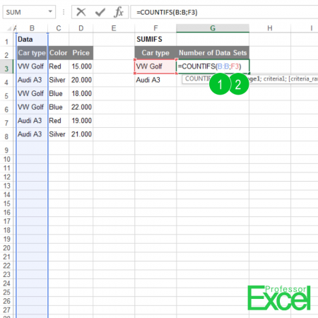
The COUNTIFS formula needs at least two parts: One search range and the criteria you are going to search for. In our example above, we got a column with car brands. You want to know how many times “VW Golf” appears (the numbers are corresponding to the picture above):
- The column which your criteria is in.
- The lookup value (in our case “VW Golf”).
- Optional: Second criteria column.
- Optional: Second lookup value
- …
Difference to COUNTIF (without “s”)
COUNTIFS is quite similar to COUNTIF (without “s”). But COUNTIF (without “s”) can only regard one criteria, whereas COUNTIFS can match up to 127 criteria.
Originally, there was only the COUNTIF formula in Excel. Since Excel 2007, Microsoft has added the version with “s” in the end in order to allow more conditions. We recommend only using the COUNTIFS formula, even if you only have one condition. That way, you only have to memorize one formula.
Solve errors with the COUNTIFS formula
- You got a wrong result, for example the returning number is not as expected?
- Make sure that all criteria ranges have the same size, for instance, column A1:A5 and B1:B5
- Are all criterias formatted correctly, e.g. numbers as numbers and text cells as text?
- You get a 0 (zero) returned, although there should be another value? Most probably, the search criteria don’t match.
- For other errors, please check out the error helper. Select your error message in the upper box and COUNTIFS in the lower one. Press ‘Solve error’ to receive more information about the error and in combination with COUNTIFS.
Special case 1: COUNTIFS horizontally
Our first special case is using the COUNTIFS formula horizontally. The search and condition ranges have a horizontal shape. The formula itself works exactly the same way like the vertical version.
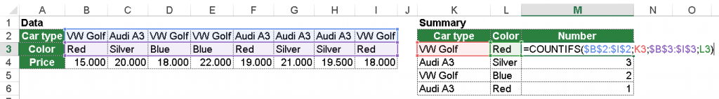
You got the table with car type as shown in the image above. Now you want to count in column M, how often you got each car and color combination in your data.
=COUNTIFS($B$2:$I$2,K3,$B$3:$I$3,L3) Let’s go through it step by step:
- The first part ($B$2:$I$2) contains the condition range of the car type. The dollar signs fix this range as you will later on copy the formula.
- The second part (K3) is the first car type – in this case “VW Golf”. This cell is not fixed with dollar signs, as you want it to change when you copy and paste the formula.
- The third part ($B$3:$I$3) contains the condition of the car color. Again, this range is fixed with the dollar signs.
- The last part (L3) is the color, in this case “Red”.
Do you want to boost your productivity in Excel?
Get the Professor Excel ribbon!

Add more than 120 great features to Excel!
Special case 2: Criteria with larger or smaller
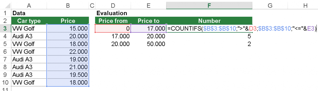
In our next example we want to count list entries with greater and smaller than certain values. In this case: We want to know, how many case there are under 17,000 EUR, between 17,000 and 20,000 EUR and above 20,000 EUR.
The trick: add “>”& and “<=”& to the formula. The complete formula in cell F3 looks like this:
=COUNTIFS($B$3:$B$10,">"&D3,$B$3:$B$10,"<="&E3)Again, let’s take a look at each part individually:
- The first condition range is the price, in this case given in range B3 to B10.
- The first condition: We want to know the number of items larger than 0 (cell D3).
- The second condition range is again the price.
- The second condition: Similar to the first condition we want to know all items also smaller than 17,000 (cell E3).

Henrik Schiffner is a freelance business consultant and software developer. He lives and works in Hamburg, Germany. Besides being an Excel enthusiast he loves photography and sports.
Summary
The Excel COUNTIFS function counts the number of occurrences of a condition or multiple conditions within a range of cells. The COUNTIFS function is useful for quickly counting instances of data within a dataset. The primary difference between the COUNTIFS function and COUNTIF function is that the COUNTIFS function can use multiple criteria while the COUNTIF function cannot.
Formula
=COUNTIFS(criteria_range1, criteria1, [criteria_range2, …)
Arguments (inputs)
criteria_range1 = the range of data to test the criteria against
criteria1 = the criteria to test against the range of data
Only one criteria range and criteria is required, but additional criteria ranges and criteria can be added if desired.
Return value
The COUNTIFS function returns the count of cells within the range that meet the criteria(s).
COUNTIFS Example

In the example above the COUNTIFS function in cell I6 counts the number of occurrences of “Jones” (from cell H6) in the range C6:C16 (the sales Representative’s names).
=COUNTIFS(C6:C16, H6)
The result is 3, because there are three instances of Jones (one in row 6, 10, and 16).
COUNTIFS with Multiple Criteria Example

The COUNTIFS function, unlike the COUNTIF function, can handle multiple criteria. In the example above the COUNTIFS function in cell J6 counts the number of occurrences of “Jones” (from cell H6) AND prices above $300 (from cell I6), in the range C6:C16 (the sales Representative’s names) and range E6:E16 (Prices), respectively. The COUNTIFS function will only count if both criteria are true.
=COUNTIFS(C6:C16, H6, E6:E16, “>”&I6))
The result is 1, because there is only one instance of Jones where the price is >$300 (in row 6).
COUNTIFS Not Blank Example
COUNTIFS can count the number of not blank cells within a range.

To count the number of not blank cells, use the not equal to operator “<>” combined with two quotes.
=COUNTIFS(G6:G25 , “<>”&””)
In the example above, the COUNTIFS function returns 15 non blank cells.
COUNTIFS Date Range Example
In this example, the COUNTIFS function can be used to count occurrences within a date range.

The COUNTIFS function in cell O6 counts the number of occurrences of orders that occur between the dates in cells M6 and N6, 1/1/2017 and 12/31/2017, respectively. Criteria 1 is greater than or equal to the date, indicated by the “>=” and the ampersand “&” connects the logical operator to the cell reference. Similarly, Criteria 2 is less than or equal to the date indicated by the “<=”.
=COUNTIFS(C6:C25, “>=”&M6 , C6:C25 , “<=”&N6)
The result is 10, because there are 10 instances in the date range between 1/1/2017 and 12/31/2017.
Additional COUNTIFS Examples
COUNTIFS greater than
To make the COUNTIFS criteria greater than, use the greater than symbol (>) in double quotes. A value or cell reference can be used with the greater than criteria.
=COUNTIFS(E6:E16, “>300”) <– Greater than 300
=COUNTIFS(E6:E16, “>”&I6) <– Greater than value in cell I6
COUNTIFS less than
To make the COUNTIFS criteria less than, use the less than symbol (<) in double quotes. A value or cell reference can be used with the less than criteria.
=COUNTIFS(E6:E16, “<200”) <– Less than 200
=COUNTIFS(E6:E16, “<“&I6) <– Less than value in cell I6
COUNTIFS not equal to
To make the COUNTIFS criteria not equal to a value, use the less than and greater than symbols (<>) in double quotes. A value or cell reference can be used with this criteria.
=COUNTIFS(E6:E16, “<>Jones”) <– Not equal to Jones
=COUNTIFS(E6:E16, “<>”&I6) <– Not equal to value in cell I6
Excel COUNTIFS (Table of Contents)
- Introduction to COUNTIFS in Excel
- How to Use COUNTIFS in Excel?
Introduction to COUNTIFS in Excel
‘COUNTIFS’ is a statistical function in Excel that is used to count cells that meet multiple criteria. The criteria could be in the form of a date, text, numbers, expression, cell reference or formula. This function applies the mentioned criteria to cells across multiple ranges and returns the count number of times the criteria are met.
COUNTIFS Function Syntax:
COUNTIFS Function Arguments:
- range1: Required represents the first range of cells that we wish to evaluate if it meets the criteria.
- criteria1: Required represents the condition or criteria to be checked/tested against each value of range1.
- range2: Optional represents the second range of cells that we wish to evaluate if it meets the criteria.
- criteria2: Required represents the condition or criteria to be checked/tested against each value of range2.
A maximum of 127 pairs of criteria and range can be entered in the function.
The number of rows and columns of each additional range provided should be the same as the first range. If there is a mismatch in the length of ranges or when the parameter supplied as criteria is a text string that is greater than 255 characters, then the function returns a #VALUE! error.
How to Use COUNTIFS in Excel?
Let’s understand how to use the COUNTIFS in Excel with a few examples.
You can download this COUNTIFS Excel Template here – COUNTIFS Excel Template
Example #1 – COUNTIFS Formula with Multiple Criteria
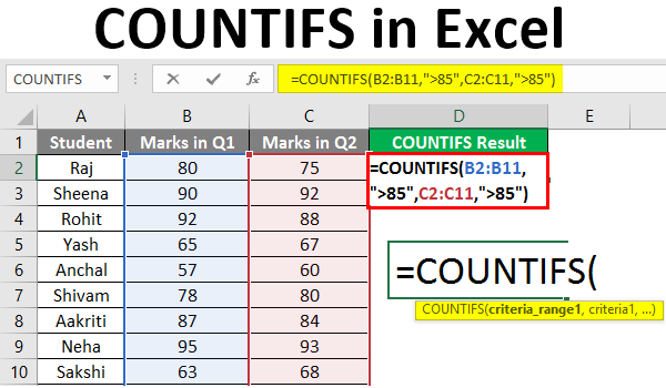
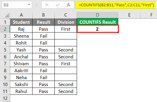
Let’s say we have the result status of a class of students, and we wish to find a count of students who has passed as well as scored ‘First Division’ marks.
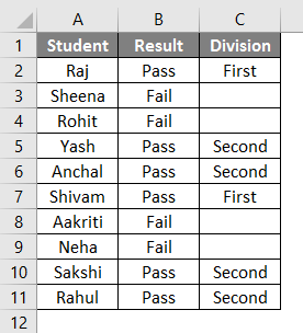
The ‘Pass/Fail’ status of students is stored in column B, and the result status according to marks, i.e. if it is ‘First Division’ or not, is stored in column C. Then the following formula tells Excel to return a count of students who has passed as well as scored ‘First Division’ marks.
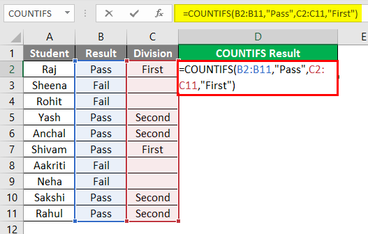
So we can see in the above screenshot that the COUNTIFS formula counts the number of students who meet both the given conditions/criteria, i.e. students who have passed as well as scored ‘First Division’ marks. The students corresponding to the below-highlighted cells will be counted to give a total count of 2, as they have passed as well as scored ‘First Division’ marks.
Example #2 – COUNTIFS Formula with the Same Criteria
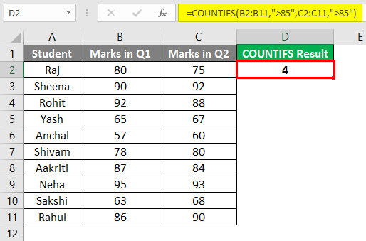
Now let’s say we have scores/marks of a class of students in the first two quarters, and we wish to find the count of students who scored more than 85 marks in both quarters. The scores of students in Quarter1 are stored in column B, and scores of students in Quarter2 are stored in column C. Then, the following formula tells Excel to return a count of students who scored more than 85 marks in both quarters.
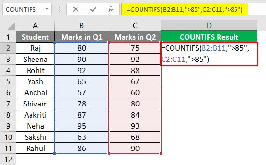
So we can see in the above screenshot that the COUNTIFS formula counts the number of students who have scored more than 85 marks in both quarters. Students corresponding to the below-highlighted cells will be counted.
Example #3 – Count Cells whose Value lie between Two Numbers
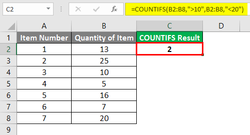
Let’s say we have two columns containing item numbers and their quantities present in a store. If we wish to find out the count of those cells or items whose quantity is between 10 and 20 (not including 10 and 20), we can use the COUNTIFS function below.
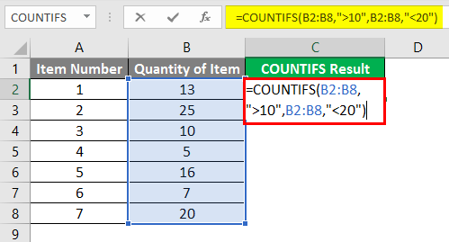
So we can see in the above screenshot that the formula counts those cells or items whose quantity is between 10 and 20. Items corresponding to the below-highlighted values will be counted to give a total count of 2.
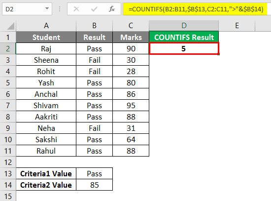
Example #4 – Criteria is a Cell Reference
Let’s say we have the result status (Pass/Fail) of a class of students and their final marks in a subject. Now, if we wish to find a count of those students who has passed as well as scored more than 85 marks, then, in this case, we use the formula as shown in the below screenshot.
So we can see in the above screenshot that in the criteria, cell reference is passed rather than supplying direct value. Concatenate (‘&’) operator is used between ‘>’ operator and cell reference address.
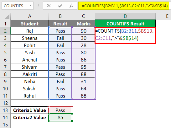
The students corresponding to the below-highlighted cells will be counted to give a total count of 5, as they meet both the conditions.
Things to Remember About COUNTIFS in Excel
- COUNTIFS is useful in cases where we wish to apply different criteria on one or more ranges, whereas COUNTIF is useful in cases where we wish to apply a single criteria on one range.
- We can use the wildcards in criteria associated with the COUNTIFS function: ‘?’ to match a single character and ‘*’ to match the sequence of characters.
- If we wish to find an actual or literal asterisk or question mark or asterisk in the range supplied, then we can use a tilde (~) in front of these wildcards ( ~*, ~?).
- If the argument provided as ‘criteria’ to the COUNTIFS function is non-numeric, then it must be enclosed in double-quotes.
- The COUNTIFS function only counts cells that meet all the specified conditions.
- Both contiguous and non-contiguous ranges are allowed in the function.
- We should try to use absolute cell references in criteria and range parameters to not break the formula when it is copied to other cells.
- COUNTIFS can also be used as a worksheet function in Excel. COUNTIFS function returns a numeric value. COUNTIFS function is not case sensitive in the case of text criteria.
- If the argument provided as ‘criteria’ to the function is a blank cell, then the function treats it like a zero value.
- The relational operators that can be used in expression criteria are:
- Less than operator: ‘<.’
- Greater than operator: ‘>.’
- Less than or Equal to the operator: ‘<=.’
- Greater than or Equal to an operator: ‘>=.’
- Equal to operator: ‘=.’
- Not Equal to operator: ‘<>.’
- Concatenate operator: ‘&’
Recommended Articles
This is a guide to COUNTIFS in Excel. Here we discuss how to use COUNTIFS in Excel along with practical examples and a downloadable excel template. You can also go through our other suggested articles –
- Count Characters in Excel
- COUNTIFS with Multiple Criteria
- COUNTA Function in Excel
- Count Formula in Excel
There are a handful of functions that we can use to count by date, month, year, or date range in Excel 365.
We can use Excel functions such as COUNTIF, COUNTIFS, SUMPRODUCT, or combinations such as IF + SUM or COUNT + FILTER for this.
But I would pick the former two functions in Excel 365. Do you know why?
Dynamic array formulas, which spill results, are one of the main attractions in Excel in Microsoft 365.
If you are looking for a dynamic array formula to count by date, month, year, and date range in Excel 365, pick none other than COUNTIF/COUNTIFS.
So, in this tutorial, let’s learn to use COUNTIF or COUNTIFS to count by date, month, year, and date range and return an array result.
Sample Records
I have extracted a few records from my daily expense spreadsheet.
Of course, I have sanitized the data to avoid sharing personal info/preferences.
So it’s just a mockup of data in Excel 365. In that, we can try to use COUNTIF and COUNTIFS to count by date, month & year, month, year, and date range.
We will try conditions (criteria) in single (non-array) and multiple (array) rows.
At one instance, we will use a helper column, and that is for the count by month (not month and year).
Sample Data:

COUNTIF to Count by a Specific Date in Excel 365
Countif Syntax: COUNTIF(range,criteria)

Non-Array Formula (Single Date)
How to search and count the number of transactions on a particular date in the above records?
Criterion/Condition: 01/06/2020 (cell F2)
Formula:-
Insert the below Excel COUNTIF formula in cell G2 to count by the specific date, i.e., 01/06/2020.
=COUNTIF(A2:A22,F2)The above Excel formula searches F2 date in A2:A22 and returns the count, i.e., 2.
Array Formula (Multiple Dates)
Can we use multiple dates (criteria) to count in the above Excel 365 formula?
Yes. Here is how.
Criteria/Conditions: 02/06/2020 (cell F4) and 01/07/2020 (cell F5).
Formula:-
Insert the below Excel COUNTIF formula in cell G4 to count by the specific dates, i.e., 02/06/2020 and 01/07/2020. It will automatically spill in G5.
=COUNTIF(A2:A22,F4:F5)COUNTIFS to Count by Month and Year in Excel 365
COUNTIFS Syntax: COUNTIFS(criteria_range1,criteria1, ...)
The functions COUNTIF and COUNTIFS in Excel 365 won’t take other functions in their ‘range’.
So we can’t use month(range)= within these two functions.
But they support other functions in the criteria part, and we will try to benefit from that feature below.

Non-Array Formula (Month and Year)
We can use COUNTIFS to count by month and year in Excel 365.
Criterion/Condition: 6 (cell F8) and 2020 (cell G8).
Formula:-
Insert the below Excel COUNTIFS formula in cell H8 to count by the above month and year.
=COUNTIFS(A2:A22,">="&DATE(G8,F8,1),A2:A22,"<="&EOMONTH(DATE(G8,F8,1),0))The DATE(G8,F8,1) formula returns 01/06/2020, and EOMONTH(DATE(G8,F8,1)) returns the last date in that month.
The count of dates between these dates will be equal to the count by month and year.
Array Formula (Months and Years)
We can use multiple months and years (criteria) in the above Excel 365 formula.
Criteria/Conditions:
- 7 (cell F10) and 2020 (cell G10).
- 7 (cell F11) and 2021 (cell G11).
Formula:-
Insert the below Excel COUNTIFS formula in cell H10 to count by the above multiple months and years.
=COUNTIFS(A2:A22,">="&DATE(G10:G11,F10:F11,1),A2:A22,"<="&EOMONTH(DATE(G10:G11,F10:F11,1),0))Array and Non-Array COUNTIFS to Count by Year in Excel 365

Assume we have the year 2020 in cell F14.
The following COUNTIFS non-array in cell G14 returns the count by the provided year in Excel 365.
=COUNTIFS(A2:A22,">="&DATE(F14,1,1),A2:A22,"<="&DATE(F14,12,31))If the year 2020 is in cell F16 and 2021 is in cell F17, then we can use the below Excel 365 dynamic array formula in cell G16.
=COUNTIFS(A2:A22,">="&DATE(F16:F17,1,1),A2:A22,"<="&DATE(F16:F17,12,31))I hope, the above two Excel formulas are self-explanatory. Let’s move to the next example.
Array and Non-Array COUNTIFS to Count by Date Range in Excel 365
In the above examples, we have learned to count the number of transactions that have taken place on a specific date, month, and year.
But what about counting the number of transactions between two dates in Excel 365?

I wish to know how many transactions I have done during 01/06/2020 (F20) and 06/06/2020 (G20).
I can use the below Excel formula in cell H20 for that.
Count by Date Range Non-Array Formula (H20):
=COUNTIFS(A2:A22,">="&F20,A2:A22,"<="&G20)What about a count by date range array formula?
Date Range 1: F22:G22
Date Range 2: F23:G23
Count by Date Range Array Formula (H22):
=COUNTIFS(A2:A22,">="&F22:F23,A2:A22,"<="&G22:G23)Array and Non-Array COUNTIFS to Count by Month Alone in Excel 365
I know this is a rare scenario.
Usually, we may include the year component in such calculations.
For example, we will usually find the number of sales in January 2020, not in both January 2020 and January 2021.
But if you are very particular to use COUNTIFS to count by month only in Excel 365, follow the below steps.
Insert the below formula in cell D2. It will substitute the year part of the dates in cell A2:A22 with the year 2021.
=DATE(2021,MONTH(A2:A22),1)It’s a dynamic array (spill) formula. So it requires a blank range in D3:D22.
You can then hide column D or keep it.
In cell K8, enter 6 which represents June.
=COUNTIFS(D2#,">="&DATE(2021,J10,1),D2#,"<="&EOMONTH(DATE(2021,J10,1),0))The above formula in cell L8 will return the count of transactions in June. It ignores the years!
What about an array formula?
Enter 6 in K10 and 7 in K11. Then, you may insert the below formula in L10.
=COUNTIFS(D2#,">="&DATE(2021,K10:K11,1),D2#,"<="&EOMONTH(DATE(2021,K10:K11,1),0))Excel 365 Resources
- Running Count Array Formula in Excel 365.
- Array Formula to Conditional Count Unique Values in Excel 365.
- Split Function Alternative in Excel 365 with Multi-Row Support.
- How to Flatten an Array in Excel 365 Using Dynamic Formulas.
- Spill Formulas to Sum Each Row in Excel 365.