Excel countif but not if

• #2

Maybe put an AND function in there as well? =COUNTIF(E4:E16, AND(«**»,NOT(«train»)))

• #3

maybe…

=COUNTIF(I11:I13,»<>TRAIN»)

• #4

Try =COUNTA(E$:E16)-COUNTIF(E4:E16,»*train*»)

• #5

maybe…

=COUNTIF(I11:I13,»<>TRAIN»)

Unfortunately, that will count blank cells as well.

If you want to ignore cells with train anywhere in the cell, you could try:
=COUNTA(E4:E16)-COUNTIF(E4:E16,»*train*»)

To only ignore cells with exactly «train», use:
=COUNTA(E4:E16)-COUNTIF(E4:E16,»train»)

• #6

Good point,

Though I assumed the poster wanted to include blanks in the count based on the logic that a blank in the range would not contain train and should be included in the count.

Either way, I appreciate you mentioning it.

• #7

maybe…

=COUNTIF(I11:I13,»<>TRAIN»)

This one did count all of the 13 cells in the array. Only two of the cells in the column were populated. Thanks

• #8

This one looks promising but I could not get it to work whichever way I tried. Thanks

• #9

Unfortunately, that will count blank cells as well.

If you want to ignore cells with train anywhere in the cell, you could try:
=COUNTA(E4:E16)-COUNTIF(E4:E16,»*train*»)

To only ignore cells with exactly «train», use:
=COUNTA(E4:E16)-COUNTIF(E4:E16,»train»)

I tried no avail. The first one came back with 4 as an answer for both columns
The second comes back with an error which I can’t fix. Correct answers were 7 and 2 for Jan 28 and Feb 18. Below is a shot of the spreadsheet. I am trying to add up the columns to show me # of populated cells without the word «train» anywhere in it. Thanks Tom

21-Jan	28-Jan	4-Feb	11-Feb	18-Feb
Fi — D
	N — D
N — D	N — D
	R — D
	R — D
	V/4400 — D			V-train
			EX-train
N — D	N&V — D			V-train
Fi — D
	N — D
4	7	0	1	2	0

<colgroup><col style=»mso-width-source:userset;mso-width-alt:2759;width:58pt» width=»78″> <col style=»mso-width-source:userset;mso-width-alt:2673;width:56pt» width=»75″> <col style=»width:49pt» span=»2″ width=»66″> <col style=»mso-width-source:userset;mso-width-alt:2360;width:50pt» width=»66″> <col style=»width:49pt» width=»66″> </colgroup><tbody>

</tbody>

• #10

…Correct answers were 7 and 2 for Jan 28 and Feb 18…

Don’t you mean 7 & 0 are the correct answers?…I copied/pasted your data into a blank spreadsheet and used =COUNTA(E2:E14)-COUNTIF(E2:E14,»*train*») and it produced the proper results (Left to Right: 4,7,0,0,0,0). Are you possibly using an explicit reference with $’s instead of without?

COUNTIF function

Use COUNTIF, one of the statistical functions, to count the number of cells that meet a criterion; for example, to count the number of times a particular city appears in a customer list.

In its simplest form, COUNTIF says:

• =COUNTIF(Where do you want to look?, What do you want to look for?)

For example:

• =COUNTIF(A2:A5,»London»)

• =COUNTIF(A2:A5,A4)

COUNTIF(range, criteria)

Argument name	Description
range    (required)	The group of cells you want to count. Range can contain numbers, arrays, a named range, or references that contain numbers. Blank and text values are ignored. Learn how to select ranges in a worksheet.
criteria    (required)	A number, expression, cell reference, or text string that determines which cells will be counted. For example, you can use a number like 32, a comparison like «>32», a cell like B4, or a word like «apples». COUNTIF uses only a single criteria. Use COUNTIFS if you want to use multiple criteria.

Examples

To use these examples in Excel, copy the data in the table below, and paste it in cell A1 of a new worksheet.

Data	Data
apples	32
oranges	54
peaches	75
apples	86
Formula	Description
=COUNTIF(A2:A5,»apples»)	Counts the number of cells with apples in cells A2 through A5. The result is 2.
=COUNTIF(A2:A5,A4)	Counts the number of cells with peaches (the value in A4) in cells A2 through A5. The result is 1.
=COUNTIF(A2:A5,A2)+COUNTIF(A2:A5,A3)	Counts the number of apples (the value in A2), and oranges (the value in A3) in cells A2 through A5. The result is 3. This formula uses COUNTIF twice to specify multiple criteria, one criteria per expression. You could also use the COUNTIFS function.
=COUNTIF(B2:B5,»>55″)	Counts the number of cells with a value greater than 55 in cells B2 through B5. The result is 2.
=COUNTIF(B2:B5,»<>»&B4)	Counts the number of cells with a value not equal to 75 in cells B2 through B5. The ampersand (&) merges the comparison operator for not equal to (<>) and the value in B4 to read =COUNTIF(B2:B5,»<>75″). The result is 3.
=COUNTIF(B2:B5,»>=32″)-COUNTIF(B2:B5,»<=85″)	Counts the number of cells with a value greater than (>) or equal to (=) 32 and less than (<) or equal to (=) 85 in cells B2 through B5. The result is 1.
=COUNTIF(A2:A5,»*»)	Counts the number of cells containing any text in cells A2 through A5. The asterisk (*) is used as the wildcard character to match any character. The result is 4.
=COUNTIF(A2:A5,»?????es»)	Counts the number of cells that have exactly 7 characters, and end with the letters «es» in cells A2 through A5. The question mark (?) is used as the wildcard character to match individual characters. The result is 2.

Common Problems

Problem	What went wrong
Wrong value returned for long strings.	The COUNTIF function returns incorrect results when you use it to match strings longer than 255 characters. To match strings longer than 255 characters, use the CONCATENATE function or the concatenate operator &. For example, =COUNTIF(A2:A5,»long string»&»another long string»).
No value returned when you expect a value.	Be sure to enclose the criteria argument in quotes.
A COUNTIF formula receives a #VALUE! error when referring to another worksheet.	This error occurs when the formula that contains the function refers to cells or a range in a closed workbook and the cells are calculated. For this feature to work, the other workbook must be open.

Best practices

Do this	Why
Be aware that COUNTIF ignores upper and lower case in text strings.	Criteria aren’t case sensitive. In other words, the string «apples» and the string «APPLES» will match the same cells.
Use wildcard characters.	Wildcard characters —the question mark (?) and asterisk (*)—can be used in criteria. A question mark matches any single character. An asterisk matches any sequence of characters. If you want to find an actual question mark or asterisk, type a tilde (~) in front of the character. For example, =COUNTIF(A2:A5,»apple?») will count all instances of «apple» with a last letter that could vary.
Make sure your data doesn’t contain erroneous characters.	When counting text values, make sure the data doesn’t contain leading spaces, trailing spaces, inconsistent use of straight and curly quotation marks, or nonprinting characters. In these cases, COUNTIF might return an unexpected value. Try using the CLEAN function or the TRIM function.
For convenience, use named ranges	COUNTIF supports named ranges in a formula (such as =COUNTIF(fruit,»>=32″)-COUNTIF(fruit,»>85″). The named range can be in the current worksheet, another worksheet in the same workbook, or from a different workbook. To reference from another workbook, that second workbook also must be open.

Note: The COUNTIF function will not count cells based on cell background or font color. However, Excel supports User-Defined Functions (UDFs) using the Microsoft Visual Basic for Applications (VBA) operations on cells based on background or font color. Here is an example of how you can Count the number of cells with specific cell color by using VBA.

Need more help?

You can always ask an expert in the Excel Tech Community or get support in the Answers community.

See also

COUNTIFS function

IF function

COUNTA function

Overview of formulas in Excel

IFS function

SUMIF function

Author: Oscar Cronquist Article last updated on September 17, 2021

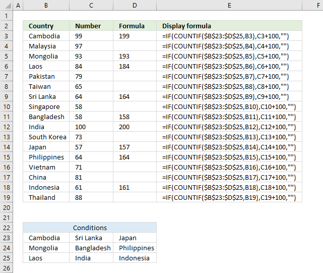
The image above demonstrates a formula that matches a value to multiple conditions, if the condition is met the formula takes the value in a corresponding cell on the same row and adds a given number.

The COUNTIF function allows you to construct a small IF formula that carries out plenty of logical expressions.

Combining the IF and COUNTIF functions also let you have more than 254 logical expressions and the effort to type the formula is minimal.

1. Use IF + COUNTIF to evaluate multiple conditions

=IF(COUNTIF($B$23:$D$25,B3),C3+100,»»)

The example shown in the above picture checks if the country in cell B3 is equal to one of the countries in cell range B23:D25.

In other words, the COUNTIF function counts how many times a specific value is found in a cell range.

If the value exists at least once in the cell range the IF function adds 100 to the value in C3. If FALSE the formula returns a blank.

Back to top

1.1 Explaining formula in cell D3

Step 1 — COUNTIF function syntax

The COUNTIF function calculates the number of cells that is equal to a condition.

COUNTIF(range, criteria)

Step 2 — Populate COUNTIF function arguments

COUNTIF(range, criteria)

becomes

COUNTIF($B$23:$D$25,B3)

range — A reference to all conditions: $B$23:$D$25

criteria — The value to match.

Step 3 — Evaluate COUNTIF function

COUNTIF($B$23:$D$25,B3)

becomes

COUNTIF({«Cambodia«, «Sri Lanka», «Japan»; «Mongolia», «Bangladesh», «Philippines»; «Laos», «India», «Indonesia»}, «Cambodia«)

and returns 1. The criteria value is found once in the array (bolded).

Step 4 — IF function syntax

The IF function returns one value if the logical test is TRUE and another value if the logical test is FALSE.

IF(logical_test, [value_if_true], [value_if_false])

Step 5 — Populate IF function arguments

IF(logical_test, [value_if_true], [value_if_false])

becomes

IF(1, C3+100, «»)

logical_test — True or False, the numerical equivalents are TRUE — 1 and False — 0 (zero). 1, in this case, is equal to TRUE.

[value_if_true] — C3+100, add 100 to value in cell C3.

[value_if_false] — «».

Step 6 — Evaluate IF function

IF(COUNTIF($B$23:$D$25, B3), C3+100, «»)

becomes

IF(1, C3+100, «»)

becomes

C3 + 100

becomes

99 + 100

and returns 199 in cell D3.

Back to top

2. Use IF + COUNTIF to evaluate multiple conditions and calculate different outcomes

The image above demonstrates a formula in cell D3 that checks if the value in cell B3 matches any of the conditions specified in cell range F4:F12. If so, add the corresponding number in cell range G4:G12 to the number in cell C3.

Formula in cell D3:

=IF(COUNTIF($F$4:$F$12, B3), C3+INDEX($G$4:$G$12, MATCH(B3, $F$4:$F$12,0)), «»)

Back to top

2.1 Explaining formula

Step 1 — Check if the value matches any of the conditions

The COUNTIF function calculates the number of cells that is equal to a condition.

COUNTIF(range, criteria)

COUNTIF($F$4:$F$12, B3)

becomes

COUNTIF({«Cambodia«; «Mongolia»; «Laos»; «Sri Lanka»; «Bangladesh»; «India»; «Japan»; «Philippines»; «Indonesia»}, «Cambodia«)

and returns 1. This means that there is one value that matches.

Step 2 — IF function

The IF function returns one value if the logical test is TRUE and another value if the logical test is FALSE.

IF(logical_test, [value_if_true], [value_if_false])

IF(COUNTIF($F$4:$F$12, B3), [value_if_true], [value_if_false])

becomes

IF(1, [value_if_true], [value_if_false])

[value_if_true] — C3+INDEX($G$4:$G$12, MATCH(B3, $F$4:$F$12,0))

[value_if_false] — «»

Step 3 — Calculate the relative position of a lookup value

The MATCH function returns the relative position of an item in an array or cell reference that matches a specified value in a specific order.

MATCH(lookup_value, lookup_array, [match_type])

MATCH(B3, $F$4:$F$12,0)

becomes

MATCH(«Cambodia», {«Cambodia»; «Mongolia»; «Laos»; «Sri Lanka»; «Bangladesh»; «India»; «Japan»; «Philippines»; «Indonesia»}, 0)

and returns 1. The lookup value is found at the first position in the array.

Step 3 — Get value

The INDEX function returns a value from a cell range, you specify which value based on a row and column number.

INDEX(array, [row_num], [column_num])

INDEX($G$4:$G$12, MATCH(B3, $F$4:$F$12,0))

becomes

INDEX($G$4:$G$12, 1)

and returns 27.

Step 4 — Add values

The plus sign lets you add numbers in an Excel formula.

C3+INDEX($G$4:$G$12, MATCH(B3, $F$4:$F$12,0))

becomes

99 + 27 equals 126.

Back to top

Get Excel *.xlsx file

Use IF + COUNTIF to perform multiple conditionsv2

Back to top

Excel has many functions where a user needs to specify a single or multiple criteria to get the result. For example, if you want to count cells based on multiple criteria, you can use the COUNTIF or COUNTIFS functions in Excel.

This tutorial covers various ways of using a single or multiple criteria in COUNTIF and COUNTIFS function in Excel.

While I will primarily be focussing on COUNTIF and COUNTIFS functions in this tutorial, all these examples can also be used in other Excel functions that take multiple criteria as inputs (such as SUMIF, SUMIFS, AVERAGEIF, and AVERAGEIFS).

An Introduction to Excel COUNTIF and COUNTIFS Functions

Let’s first get a grip on using COUNTIF and COUNTIFS functions in Excel.

Excel COUNTIF Function (takes Single Criteria)

Excel COUNTIF function is best suited for situations when you want to count cells based on a single criterion. If you want to count based on multiple criteria, use COUNTIFS function.

Syntax

=COUNTIF(range, criteria)

Input Arguments

• range –  the range of cells which you want to count.
• criteria – the criteria that must be evaluated against the range of cells for a cell to be counted.

Excel COUNTIFS Function (takes Multiple Criteria)

Excel COUNTIFS function is best suited for situations when you want to count cells based on multiple criteria.

Syntax

=COUNTIFS(criteria_range1, criteria1, [criteria_range2, criteria2]…)

Input Arguments

• criteria_range1 – The range of cells for which you want to evaluate against criteria1.
• criteria1 – the criteria which you want to evaluate for criteria_range1 to determine which cells to count.
• [criteria_range2] – The range of cells for which you want to evaluate against criteria2.
• [criteria2] – the criteria which you want to evaluate for criteria_range2 to determine which cells to count.

Now let’s have a look at some examples of using multiple criteria in COUNTIF functions in Excel.

Using NUMBER Criteria in Excel COUNTIF Functions

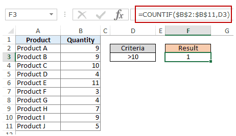
#1 Count Cells when Criteria is EQUAL to a Value

To get the count of cells where the criteria argument is equal to a specified value, you can either directly enter the criteria or use the cell reference that contains the criteria.

Below is an example where we count the cells that contain the number 9 (which means that the criteria argument is equal to 9). Here is the formula:

=COUNTIF($B$2:$B$11,D3)

In the above example (in the pic), the criteria is in cell D3. You can also enter the criteria directly into the formula. For example, you can also use:

=COUNTIF($B$2:$B$11,9)

#2 Count Cells when Criteria is GREATER THAN a Value

To get the count of cells with a value greater than a specified value, we use the greater than operator (“>”). We could either use it directly in the formula or use a cell reference that has the criteria.

Whenever we use an operator in criteria in Excel, we need to put it within double quotes. For example, if the criteria is greater than 10, then we need to enter “>10” as the criteria (see pic below):

Here is the formula:

=COUNTIF($B$2:$B$11,”>10″)

You can also have the criteria in a cell and use the cell reference as the criteria. In this case, you need NOT put the criteria in double quotes:

=COUNTIF($B$2:$B$11,D3)

There could also be a case when you want the criteria to be in a cell, but don’t want it with the operator. For example, you may want the cell D3 to have the number 10 and not >10.

In that case, you need to create a criteria argument which is a combination of operator and cell reference (see pic below):

=COUNTIF($B$2:$B$11,”>”&D3)

NOTE: When you combine an operator and a cell reference, the operator is always in double quotes. The operator and cell reference are joined by an ampersand (&).

#3 Count Cells when Criteria is LESS THAN a Value

To get the count of cells with a value less than a specified value, we use the less than operator (“<“). We could either use it directly in the formula or use a cell reference that has the criteria.

Whenever we use an operator in criteria in Excel, we need to put it within double quotes. For example, if the criterion is that the number should be less than 5, then we need to enter “<5” as the criteria (see pic below):

=COUNTIF($B$2:$B$11,”<5″)

You can also have the criteria in a cell and use the cell reference as the criteria. In this case, you need NOT put the criteria in double quotes (see pic below):

=COUNTIF($B$2:$B$11,D3)

Also, there could be a case when you want the criteria to be in a cell, but don’t want it with the operator. For example, you may want the cell D3 to have the number 5 and not <5.

In that case, you need to create a criteria argument which is a combination of operator and cell reference:

=COUNTIF($B$2:$B$11,”<“&D3)

NOTE: When you combine an operator and a cell reference, the operator is always in double quotes. The operator and cell reference are joined by an ampersand (&).

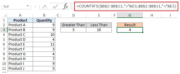
#4 Count Cells with Multiple Criteria – Between Two Values

To get a count of values between two values, we need to use multiple criteria in the COUNTIF function.

Here are two methods of doing this:

METHOD 1: Using COUNTIFS function

COUNTIFS function can handle multiple criteria as arguments and counts the cells only when all the criteria are TRUE. To count cells with values between two specified values (say 5 and 10), we can use the following COUNTIFS function:

=COUNTIFS($B$2:$B$11,”>5″,$B$2:$B$11,”<10″)

NOTE: The above formula does not count cells that contain 5 or 10. If you want to include these cells, use greater than equal to (>=) and less than equal to (<=) operators. Here is the formula:

=COUNTIFS($B$2:$B$11,”>=5″,$B$2:$B$11,”<=10″) 

You can also have these criteria in cells and use the cell reference as the criteria. In this case, you need NOT put the criteria in double quotes (see pic below):

You can also use a combination of cells references and operators (where the operator is entered directly in the formula). When you combine an operator and a cell reference, the operator is always in double quotes. The operator and cell reference are joined by an ampersand (&).

METHOD 2: Using two COUNTIF functions

If you have multiple criteria, you can either use COUNTIFS or create a combination of COUNTIF functions. The formula below would also do the same thing:

=COUNTIF($B$2:$B$11,”>5″)-COUNTIF($B$2:$B$11,”>10″)

In the above formula, we first find the number of cells that have a value greater than 5 and we subtract the count of cells with a value greater than 10. This would give us the result as 5 (which is the number of cells that have values more than 5 and less than equal to 10).

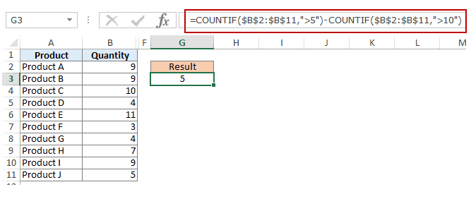
If you want the formula to include both 5 and 10, use the following formula instead:

=COUNTIF($B$2:$B$11,”>=5″)-COUNTIF($B$2:$B$11,”>10″)

If you want the formula to exclude both ‘5’ and ’10’ from the counting, use the following formula:

=COUNTIF($B$2:$B$11,”>=5″)-COUNTIF($B$2:$B$11,”>10″)-COUNTIF($B$2:$B$11,10)

You can have these criteria in cells and use the cells references, or you can use a combination of operators and cells references.

Using TEXT Criteria in Excel Functions

#1 Count Cells when Criteria is EQUAL to a Specified text

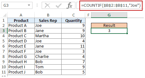
To count cells that contain an exact match of the specified text, we can simply use that text as the criteria. For example, in the dataset (shown below in the pic), if I want to count all the cells with the name Joe in it, I can use the below formula:

=COUNTIF($B$2:$B$11,”Joe”)

Since this is a text string, I need to put the text criteria in double quotes.

You can also have the criteria in a cell and then use that cell reference (as shown below):

=COUNTIF($B$2:$B$11,E3)

NOTE: You can get wrong results if there are leading/trailing spaces in the criteria or criteria range. Make sure you clean the data before using these formulas.

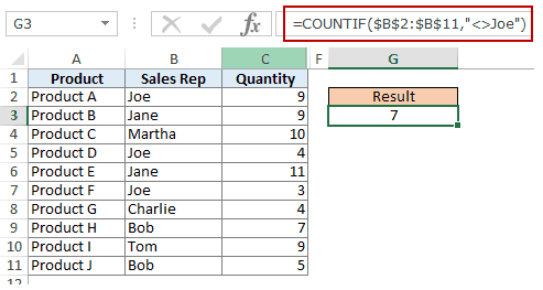
#2 Count Cells when Criteria is NOT EQUAL to a Specified text

Similar to what we saw in the above example, you can also count cells that do not contain a specified text. To do this, we need to use the not equal to operator (<>).

Suppose you want to count all the cells that do not contain the name JOE, here is the formula that will do it:

=COUNTIF($B$2:$B$11,”<>Joe”)

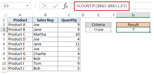
You can also have the criteria in a cell and use the cell reference as the criteria. In this case, you need NOT put the criteria in double quotes (see pic below):

=COUNTIF($B$2:$B$11,E3)

There could also be a case when you want the criteria to be in a cell but don’t want it with the operator. For example, you may want the cell D3 to have the name Joe and not <>Joe.

In that case, you need to create a criteria argument which is a combination of operator and cell reference (see pic below):

=COUNTIF($B$2:$B$11,”<>”&E3)

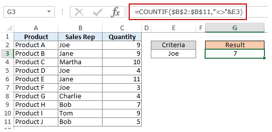
When you combine an operator and a cell reference, the operator is always in double quotes. The operator and cell reference are joined by an ampersand (&).

Using DATE Criteria in Excel COUNTIF and COUNTIFS Functions

Excel store date and time as numbers. So we can use it the same way we use numbers.

#1 Count Cells when Criteria is EQUAL to a Specified Date

To get the count of cells that contain the specified date, we would use the equal to operator (=) along with the date.

To use the date, I recommend using the DATE function, as it gets rid of any possibility of error in the date value. So, for example, if I want to use the date September 1, 2015, I can use the DATE function as shown below:

=DATE(2015,9,1)

This formula would return the same date despite regional differences. For example, 01-09-2015 would be September 1, 2015 according to the  US date syntax and January 09, 2015 according to the UK date syntax. However, this formula would always return September 1, 2105.

Here is the formula to count the number of cells that contain the date 02-09-2015:

=COUNTIF($A$2:$A$11,DATE(2015,9,2))

#2 Count Cells when Criteria is BEFORE or AFTER to a Specified Date

To count cells that contain date before or after a specified date, we can use the less than/greater than operators.

For example, if I want to count all the cells that contain a date that is after September 02, 2015, I can use the formula:

=COUNTIF($A$2:$A$11,”>”&DATE(2015,9,2))

Similarly, you can also count the number of cells before a specified date. If you want to include a date in the counting, use and ‘equal to’ operator along with ‘greater than/less than’ operator.

You can also use a cell reference that contains a date. In this case, you need to combine the operator (within double quotes) with the date using an ampersand (&).

See example below:

=COUNTIF($A$2:$A$11,”>”&F3)

#3 Count Cells with Multiple Criteria – Between Two Dates

To get a count of values between two values, we need to use multiple criteria in the COUNTIF function.

We can do this using two methods – One single COUNTIFS function or two COUNTIF functions.

METHOD 1: Using COUNTIFS function

COUNTIFS function can take multiple criteria as the arguments and counts the cells only when all the criteria are TRUE. To count cells with values between two specified dates (say September 2 and September 7), we can use the following COUNTIFS function:

=COUNTIFS($A$2:$A$11,”>”&DATE(2015,9,2),$A$2:$A$11,”<“&DATE(2015,9,7))

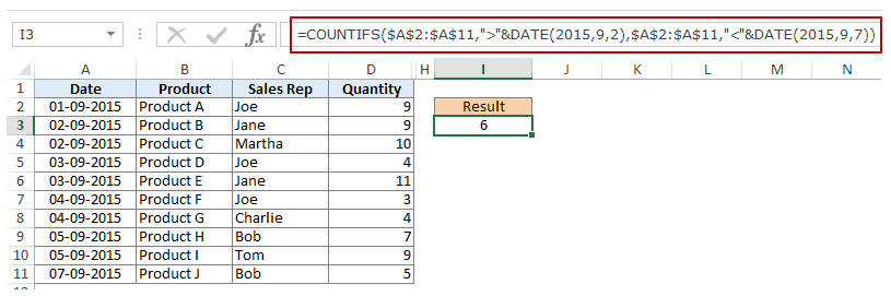
The above formula does not count cells that contain the specified dates. If you want to include these dates as well, use greater than equal to (>=) and less than equal to (<=) operators. Here is the formula:

=COUNTIFS($A$2:$A$11,”>=”&DATE(2015,9,2),$A$2:$A$11,”<=”&DATE(2015,9,7))

You can also have the dates in a cell and use the cell reference as the criteria. In this case, you can not have the operator with the date in the cells. You need to manually add operators in the formula (in double quotes) and add cell reference using an ampersand (&). See the pic below:

=COUNTIFS($A$2:$A$11,”>”&F3,$A$2:$A$11,”<“&G3)

METHOD 2: Using COUNTIF functions

If you have multiple criteria, you can either use one COUNTIFS function or create a combination of two COUNTIF functions. The formula below would also do the trick:

=COUNTIF($A$2:$A$11,”>”&DATE(2015,9,2))-COUNTIF($A$2:$A$11,”>”&DATE(2015,9,7))

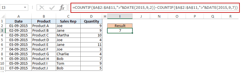
In the above formula, we first find the number of cells that have a date after September 2 and we subtract the count of cells with dates after September 7. This would give us the result as 7 (which is the number of cells that have dates after September 2 and on or before September 7).

If you don’t want the formula to count both September 2 and September 7, use the following formula instead:

=COUNTIF($A$2:$A$11,”>=”&DATE(2015,9,2))-COUNTIF($A$2:$A$11,”>”&DATE(2015,9,7))

If you want to exclude both the dates from counting, use the following formula:

=COUNTIF($A$2:$A$11,”>”&DATE(2015,9,2))-COUNTIF($A$2:$A$11,”>”&DATE(2015,9,7)-COUNTIF($A$2:$A$11,DATE(2015,9,7)))

Also, you can have the criteria dates in cells and use the cells references (along with operators in double quotes joined using ampersand).

Using WILDCARD CHARACTERS in Criteria in COUNTIF & COUNTIFS Functions

There are three wildcard characters in Excel:

1. * (asterisk) – It represents any number of characters. For example, ex* could mean excel, excels, example, expert, etc.
2. ? (question mark) – It represents one single character. For example, Tr?mp could mean Trump or Tramp.
3. ~ (tilde) – It is used to identify a wildcard character (~, *, ?) in the text.

You can use COUNTIF function with wildcard characters to count cells when other inbuilt count function fails. For example, suppose you have a data set as shown below:

Now let’s take various examples:

#1 Count Cells that contain Text

To count cells with text in it, we can use the wildcard character * (asterisk). Since asterisk represents any number of characters, it would count all cells that have any text in it. Here is the formula:

=COUNTIFS($C$2:$C$11,”*”)

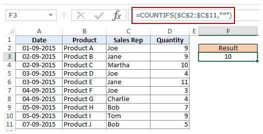
Note: The formula above ignores cells that contain numbers, blank cells, and logical values, but would count the cells contain an apostrophe (and hence appear blank) or cells that contain empty string (=””) which may have been returned as a part of a formula.

Here is a detailed tutorial on handling cases where there is an empty string or apostrophe.

Here is a detailed tutorial on handling cases where there are empty strings or apostrophes.

Below is a video that explains different scenarios of counting cells with text in it.

#2 Count Non-blank Cells

If you are thinking of using COUNTA function, think again.

Try it and it might fail you. COUNTA will also count a cell that contains an empty string (often returned by formulas as =”” or when people enter only an apostrophe in a cell). Cells that contain empty strings look blank but are not, and thus counted by the COUNTA function.

COUNTA will also count a cell that contains an empty string (often returned by formulas as =”” or when people enter only an apostrophe in a cell). Cells that contain empty strings look blank but are not, and thus counted by the COUNTA function.

So if you use the formula =COUNTA(A1:A11), it returns 11, while it should return 10.

Here is the fix:

=COUNTIF($A$1:$A$11,”?*”)+COUNT($A$1:$A$11)+SUMPRODUCT(–ISLOGICAL($A$1:$A$11))

Let’s understand this formula by breaking it down:

#3 Count Cells that contain specific text

Let’s say we want to count all the cells where the sales rep name begins with J. This can easily be achieved by using a wildcard character in COUNTIF function. Here is the formula:

=COUNTIFS($C$2:$C$11,”J*”) 

The criteria J* specifies that the text in a cell should begin with J and can contain any number of characters.

If you want to count cells that contain the alphabet anywhere in the text, flank it with an asterisk on both sides. For example, if you want to count cells that contain the alphabet “a” in it, use *a* as the criteria.

This article is unusually long compared to my other articles. Hope you have enjoyed it. Let me know your thoughts by leaving a comment.

You May Also Find the following Excel tutorials useful:

• Count the number of words in Excel.
• Count Cells Based on Background Color in Excel.
• How to Sum a Column in Excel (5 Really Easy Ways)

СЧЕТЕСЛИ в Excel — примеры функции с одним и несколькими условиями

В этой статье мы сосредоточимся на функции Excel СЧЕТЕСЛИ (COUNTIF в английском варианте), которая предназначена для подсчета ячеек с определённым условием. Сначала мы кратко рассмотрим синтаксис и общее использование, а затем я приведу ряд примеров и предупрежу о возможных причудах при подсчете по нескольким критериям одновременно или же с определёнными типами данных.

По сути,они одинаковы во всех версиях, поэтому вы можете использовать примеры в MS Excel 2016, 2013, 2010 и 2007.

1. Примеры работы функции СЧЕТЕСЛИ.
   • Для подсчета текста.
   • Подсчет ячеек, начинающихся или заканчивающихся определенными символами
   • Подсчет чисел по условию.
   • Примеры с датами.
2. Как посчитать количество пустых и непустых ячеек?
3. Нулевые строки.
4. СЧЕТЕСЛИ с несколькими условиями.
   • Количество чисел в диапазоне
   • Количество ячеек с несколькими условиями ИЛИ.
5. Использование СЧЕТЕСЛИ для подсчета дубликатов.
   • 1. Ищем дубликаты в одном столбце
   • 2. Сколько совпадений между двумя столбцами?
   • 3. Сколько дубликатов и уникальных значений в строке?
6. Часто задаваемые вопросы и проблемы.

Функция Excel СЧЕТЕСЛИ применяется для подсчета количества ячеек в указанном диапазоне, которые соответствуют определенному условию.

Например, вы можете воспользоваться ею, чтобы узнать, сколько ячеек в вашей рабочей таблице содержит число, больше или меньше указанной вами величины. Другое стандартное использование — для подсчета ячеек с определенным словом или с определенной буквой (буквами).

СЧЕТЕСЛИ(диапазон; критерий)

Как видите, здесь только 2 аргумента, оба из которых являются обязательными:

• диапазон — определяет одну или несколько клеток для подсчета. Вы помещаете диапазон в формулу, как обычно, например, A1: A20.
• критерий — определяет условие, которое определяет, что именно считать. Это может быть число, текстовая строка, ссылка или выражение. Например, вы можете употребить  следующие критерии: «10», A2, «> = 10», «какой-то текст».

Что нужно обязательно запомнить?

• В аргументе «критерий» условие всегда нужно записывать в кавычках, кроме случая, когда используется ссылка либо какая-то функция.
• Любой из аргументов ссылается на диапазон из другой книги Excel, то эта книга должна быть открыта.
• Регистр букв не учитывается.
• Также можно применить знаки подстановки * и ? (о них далее – подробнее).
• Чтобы избежать ошибок, в тексте не должно быть непечатаемых знаков.

Как видите, синтаксис очень прост. Однако, он допускает множество возможных вариаций условий, в том числе символы подстановки, значения других ячеек и даже другие функции Excel. Это разнообразие делает функцию СЧЕТЕСЛИ действительно мощной и пригодной для многих задач, как вы увидите в следующих примерах.

Примеры работы функции СЧЕТЕСЛИ.

Для подсчета текста.

Давайте разбираться, как это работает. На рисунке ниже вы видите список заказов, выполненных менеджерами. Выражение  =СЧЕТЕСЛИ(В2:В22,»Никитенко») подсчитывает, сколько раз этот работник присутствует в списке:

Замечание. Критерий не чувствителен к регистру букв, поэтому можно вводить как прописные, так и строчные буквы.

Если ваши данные содержат несколько вариантов слов, которые вы хотите сосчитать, то вы можете использовать подстановочные знаки для подсчета всех ячеек, содержащих определенное слово, фразу или буквы, как часть их содержимого.

К примеру, в нашей таблице есть несколько заказчиков «Корона» из разных городов. Нам необходимо подсчитать общее количество заказов «Корона» независимо от города.

=СЧЁТЕСЛИ(A2:A22;»*Коро*»)

Мы подсчитали количество заказов, где в наименовании заказчика встречается «коро» в любом регистре. Звездочка (*) используется для поиска ячеек с любой последовательностью начальных и конечных символов, как показано в приведенном выше примере. Если вам нужно заменить какой-либо один символ, введите вместо него знак вопроса (?).

Кроме того, указывать условие прямо в формуле не совсем рационально, так как при необходимости подсчитать какие-то другие значения вам придется корректировать её. А это не слишком удобно.

Рекомендуется условие записывать в какую-либо ячейку и затем ссылаться на нее. Так мы сделали в H9. Также можно употребить подстановочные знаки со ссылками с помощью оператора конкатенации (&). Например, вместо того, чтобы указывать «* Коро *» непосредственно в формуле, вы можете записать его куда-нибудь, и использовать следующую конструкцию для подсчета ячеек, содержащих «Коро»:

=СЧЁТЕСЛИ(A2:A22;»*»&H8&»*»)

Подсчет ячеек, начинающихся или заканчивающихся определенными символами

Вы можете употребить подстановочный знак звездочку (*) или знак вопроса (?) в зависимости от того, какого именно результата вы хотите достичь.

Если вы хотите узнать количество ячеек, которые начинаются или заканчиваются определенным текстом, независимо от того, сколько имеется других символов, используйте:

=СЧЁТЕСЛИ(A2:A22;»К*») — считать значения, которые начинаются с « К» .

=СЧЁТЕСЛИ(A2:A22;»*р») — считать заканчивающиеся буквой «р».

Если вы ищете количество ячеек, которые начинаются или заканчиваются определенными буквами и содержат точное количество символов, то поставьте вопросительный знак (?):

=СЧЁТЕСЛИ(С2:С22;»????д») — находит количество буквой «д» в конце и текст в которых состоит из 5 букв, включая пробелы.

= СЧЁТЕСЛИ(С2:С22,»??») — считает количество состоящих из 2 символов, включая пробелы.

Примечание. Чтобы узнать количество клеток, содержащих в тексте знак вопроса или звездочку, введите тильду (~) перед символом ? или *.

Например, = СЧЁТЕСЛИ(С2:С22,»*~?*») будут подсчитаны все позиции, содержащие знак вопроса в диапазоне С2:С22.

Подсчет чисел по условию.

В отношении чисел редко случается, что нужно подсчитать количество их, равных какому-то определённому числу. Тем не менее, укажем, что записать нужно примерно следующее:

= СЧЁТЕСЛИ(D2:D22,10000)

Гораздо чаще нужно высчитать количество значений, больших либо меньших определенной величины.

Чтобы подсчитать значения, которые больше, меньше или равны указанному вами числу, вы просто добавляете соответствующий критерий, как показано в таблице ниже.

Обратите внимание, что математический оператор вместе с числом всегда заключен в кавычки .

критерии		Описание
Если больше, чем	=СЧЕТЕСЛИ(А2:А10;»>5″)	Подсчитайте, где значение больше 5.
Если меньше чем	=СЧЕТЕСЛИ(А2:А10;»>5″)	Подсчет со числами менее 5.
Если равно	=СЧЕТЕСЛИ(А2:А10;»=5″)	Определите, сколько раз значение равно 5.
Если не равно	=СЧЕТЕСЛИ(А2:А10;»<>5″)	Подсчитайте, сколько раз не равно 5.
Если больше или равно	=СЧЕТЕСЛИ(А2:А10;»>=5″)	Подсчет, когда больше или равно 5.
Если меньше или равно	=СЧЕТЕСЛИ(А2:А10;»<=5″)	Подсчет, где меньше или равно 5.

В нашем примере

=СЧЁТЕСЛИ(D2:D22;»>10000″)

Считаем количество крупных заказов на сумму более 10 000. Обратите внимание, что условие подсчета мы записываем здесь в виде текстовой строки и поэтому заключаем его в двойные кавычки.

Вы также можете использовать все вышеприведенные варианты для подсчета ячеек на основе значения другой ячейки. Вам просто нужно заменить число ссылкой.

Замечание. В случае использования ссылки, вы должны заключить математический оператор в кавычки и добавить амперсанд (&) перед ним. Например, чтобы подсчитать числа в диапазоне D2: D9, превышающие D3, используйте =СЧЕТЕСЛИ(D2:D9,»>»&D3)

Если вы хотите сосчитать записи, которые содержат математический оператор, как часть их содержимого, то есть символ «>», «<» или «=», то употребите в условиях подстановочный знак с оператором. Такие критерии будут рассматриваться как текстовая строка, а не числовое выражение.

Например, =СЧЕТЕСЛИ(D2:D9,»*>5*») будет подсчитывать все позиции в диапазоне D2: D9 с таким содержимым, как «Доставка >5 дней» или «>5 единиц в наличии».

Примеры с датами.

Если вы хотите сосчитать клетки с датами, которые больше, меньше или равны указанной вами дате, вы можете воспользоваться уже знакомым способом, используя формулы, аналогичные тем, которые мы обсуждали чуть выше. Все вышеприведенное работает как для дат, так и для чисел.

Позвольте привести несколько примеров:

критерии		Описание
Даты, равные указанной дате.	=СЧЕТЕСЛИ(E2:E22;»01.02.2019″)	Подсчитывает количество ячеек в диапазоне E2:E22 с датой 1 июня 2014 года.
Даты больше или равные другой дате.	=СЧЕТЕСЛИ(E2:E22,»>=01.02.2019″)	Сосчитайте количество ячеек в диапазоне E2:E22 с датой, большей или равной 01.06.2014.
Даты, которые больше или равны дате в другой ячейке, минус X дней.	=СЧЕТЕСЛИ(E2:E22,»>=»&H2-7)	Определите количество ячеек в диапазоне E2:E22 с датой, большей или равной дате в H2, минус 7 дней.

Помимо этих стандартных способов, вы можете употребить функцию СЧЕТЕСЛИ в сочетании с функциями даты и времени, например, СЕГОДНЯ(), для подсчета ячеек на основе текущей даты.

критерии
Равные текущей дате.	=СЧЕТЕСЛИ(E2:E22;СЕГОДНЯ())
До текущей даты, то есть меньше, чем сегодня.	=СЧЕТЕСЛИ(E2:E22;»<«&СЕГОДНЯ())
После текущей даты, т.е. больше, чем сегодня.	=СЧЕТЕСЛИ(E2:E22;»>»& ЕГОДНЯ ())
Даты, которые должны наступить через неделю.	= СЧЕТЕСЛИ(E2:E22,»=»&СЕГОДНЯ()+7)
В определенном диапазоне времени.	=СЧЁТЕСЛИ(E2:E22;»>=»&СЕГОДНЯ()+30)-СЧЁТЕСЛИ(E2:E22;»>»&СЕГОДНЯ())

Как посчитать количество пустых и непустых ячеек?

Посмотрим, как можно применить функцию СЧЕТЕСЛИ в Excel для подсчета количества пустых или непустых ячеек в указанном диапазоне.

Непустые.

В некоторых руководствах по работе с СЧЕТЕСЛИ вы можете встретить предложения для подсчета непустых ячеек, подобные этому:

СЧЕТЕСЛИ(диапазон;»*»)

Но дело в том, что приведенное выше выражение подсчитывает только клетки, содержащие любые текстовые значения. А это означает, что те из них, что включают даты и числа, будут обрабатываться как пустые (игнорироваться) и не войдут в общий итог!

Если вам нужно универсальное решение для подсчета всех непустых ячеек в указанном диапазоне, то введите:

СЧЕТЕСЛИ(диапазон;»<>» & «»)

Это корректно работает со всеми типами значений — текстом, датами и числами — как вы можете видеть на рисунке ниже.

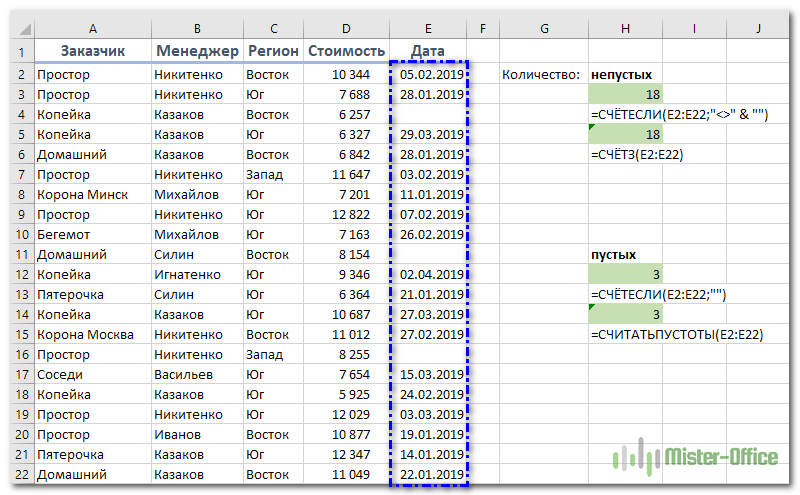
Также непустые ячейки в диапазоне можно подсчитать:

=СЧЁТЗ(E2:E22).

Пустые.

Если вы хотите сосчитать пустые позиции в определенном диапазоне, вы должны придерживаться того же подхода — используйте в условиях символ подстановки для текстовых значений и параметр “” для подсчета всех пустых ячеек.

Считаем клетки, не содержащие текст:

СЧЕТЕСЛИ( диапазон; «<>» & «*»)

Поскольку звездочка (*) соответствует любой последовательности текстовых символов, в расчет принимаются клетки, не равные *, т.е. не содержащие текста в указанном диапазоне.

Для подсчета пустых клеток (все типы значений):

=СЧЁТЕСЛИ(E2:E22;»»)

Конечно, для таких случаев есть и специальная функция

=СЧИТАТЬПУСТОТЫ(E2:E22)

Но не все знают о ее существовании. Но вы теперь в курсе …

Нулевые строки.

Также имейте в виду, что СЧЕТЕСЛИ и СЧИТАТЬПУСТОТЫ считают ячейки с пустыми строками, которые только на первый взгляд выглядят пустыми.

Что такое эти пустые строки? Они также часто возникают при импорте данных из других программ (например, 1С). Внешне в них ничего нет, но на самом деле это не так. Если попробовать найти такие «пустышки» (F5 -Выделить — Пустые ячейки) — они не определяются. Но фильтр данных при этом их видит как пустые и фильтрует как пустые.

Дело в том, что существует такое понятие, как «строка нулевой длины» (или «нулевая строка»). Нулевая строка возникает, когда программе нужно вставить какое-то значение, а вставить нечего.

Проблемы начинаются тогда, когда вы пытаетесь с ней произвести какие-то математические вычисления (вычитание, деление, умножение и т.д.). Получите сообщение об ошибке #ЗНАЧ!. При этом функции СУММ и СЧЕТ их игнорируют, как будто там находится текст. А внешне там его нет.

И самое интересное — если указать на нее мышкой и нажать Delete (или вкладка Главная — Редактирование — Очистить содержимое) — то она становится действительно пустой, и с ней начинают работать формулы и другие функции Excel без всяких ошибок.

Если вы не хотите рассматривать их как пустые, используйте для подсчета реально пустых клеток следующее выражение:

=ЧСТРОК(E2:E22)*ЧИСЛСТОЛБ(E2:E22)-СЧЁТЕСЛИ(E2:E22;»<>»&»»)

Откуда могут появиться нулевые строки в ячейках? Здесь может быть несколько вариантов:

1. Он есть там изначально, потому что именно так настроена выгрузка и создание файлов в сторонней программе (вроде 1С). В некоторых случаях такие выгрузки настроены таким образом, что как таковых пустых ячеек нет — они просто заполняются строкой нулевой длины.
2. Была создана формула, результатом которой стал текст нулевой длины. Самый простой случай:

=ЕСЛИ(Е1=1;10;»»)

В итоге, если в Е1 записано что угодно, отличное от 1, программа вернет строку нулевой длины. И если впоследствии формулу заменять значением (Специальная вставка – Значения), то получим нашу псевдо-пустую позицию.

Если вы проверяете какие-то условия при помощи функции ЕСЛИ и в дальнейшем планируете производить с результатами математические действия, то лучше вместо «» ставьте 0. Тогда проблем не будет. Нули всегда можно заменить или скрыть: Файл -Параметры -Дополнительно — Показывать нули в позициях, которые содержат нулевые значения.

СЧЕТЕСЛИ с несколькими условиями.

На самом деле функция Эксель СЧЕТЕСЛИ не предназначена для расчета количества ячеек по нескольким условиям. В большинстве случаев я рекомендую использовать его множественный аналог — функцию СЧЕТЕСЛИМН. Она как раз и предназначена для вычисления количества ячеек, которые соответствуют двум или более условиям (логика И). Однако, некоторые задачи могут быть решены путем объединения двух или более функций СЧЕТЕСЛИ в одно выражение.

Количество чисел в диапазоне

Одним из наиболее распространенных применений функции СЧЕТЕСЛИ с двумя критериями является определение количества чисел в определенном интервале, т.е. меньше X, но больше Y.

Например, вы можете использовать для вычисления ячеек в диапазоне B2: B9, где значение больше 5 и меньше или равно 15:

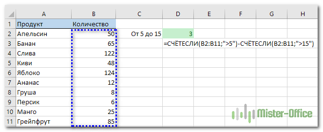
=СЧЁТЕСЛИ(B2:B11;»>5″)-СЧЁТЕСЛИ(B2:B11;»>15″)

Количество ячеек с несколькими условиями ИЛИ.

Когда вы хотите найти количество нескольких различных элементов в диапазоне, добавьте 2 или более функций СЧЕТЕСЛИ в выражение. Предположим, у вас есть список покупок, и вы хотите узнать, сколько в нем безалкогольных напитков.

Сделаем это:

=СЧЁТЕСЛИ(A4:A13;»Лимонад»)+СЧЁТЕСЛИ(A2:A11;»*сок»)

Обратите внимание, что мы включили подстановочный знак (*) во второй критерий. Он используется для вычисления количества всех видов сока в списке.

Как вы понимаете, сюда можно добавить и больше условий.

Использование СЧЕТЕСЛИ для подсчета дубликатов.

Другое возможное использование функции СЧЕТЕСЛИ в Excel — для поиска дубликатов в одном столбце, между двумя столбцами или в строке.

1. Ищем дубликаты в одном столбце

Эта простое выражение СЧЁТЕСЛИ($A$2:$A$24;A2)>1 найдет все одинаковые записи в A2: A24.

А другая формула СЧЁТЕСЛИ(B2:B24;ИСТИНА) сообщит вам, сколько существует дубликатов:

Для более наглядного представления найденных совпадений я использовал условное форматирование значения ИСТИНА.

2. Сколько совпадений между двумя столбцами?

Сравним список2 со списком1. В столбце Е берем последовательно каждое значение из списка2 и считаем, сколько раз оно встречается в списке1. Если совпадений ноль, значит это уникальное значение. На рисунке такие выделены цветом при помощи условного форматирования.

Выражение  =СЧЁТЕСЛИ($A$2:$A$24;C2) копируем вниз по столбцу Е.

Аналогичный расчет можно сделать и наоборот – брать значения из первого списка и искать дубликаты во втором.

Для того, чтобы просто определить количество дубликатов, можно использовать комбинацию функций СУММПРОИЗВ и СЧЕТЕСЛИ.

=СУММПРОИЗВ((СЧЁТЕСЛИ(A2:A24;C2:C24)>0)*(C2:C24<>»»))

Подсчитаем количество уникальных значений в списке2:

=СУММПРОИЗВ((СЧЁТЕСЛИ(A2:A24;C2:C24)=0)*(C2:C24<>»»))

Получаем 7 уникальных записей и 16 дубликатов, что и видно на рисунке.

Полезное. Если вы хотите выделить дублирующиеся позиции или целые строки, содержащие повторяющиеся записи, вы можете создать правила условного форматирования на основе формул СЧЕТЕСЛИ, как показано в этом руководстве — правила условного форматирования Excel.

3. Сколько дубликатов и уникальных значений в строке?

Если нужно сосчитать дубликаты или уникальные значения в определенной строке, а не в столбце, используйте одну из следующих формул. Они могут быть полезны, например, для анализа истории розыгрыша лотереи.

Считаем количество дубликатов:

=СУММПРОИЗВ((СЧЁТЕСЛИ(A2:K2;A2:K2)>1)*(A2:K2<>»»))

Видим, что 13 выпадало 2 раза.

Подсчитать уникальные значения:

=СУММПРОИЗВ((СЧЁТЕСЛИ(A2:K2;A2:K2)=1)*(A2:K2<>»»))

Часто задаваемые вопросы и проблемы.

Я надеюсь, что эти примеры помогли вам почувствовать функцию Excel СЧЕТЕСЛИ. Если вы попробовали какую-либо из приведенных выше формул в своих данных и не смогли заставить их работать или у вас возникла проблема, взгляните на следующие 5 наиболее распространенных проблем. Есть большая вероятность, что вы найдете там ответ или же полезный совет.

1. Возможен ли подсчет в несмежном диапазоне клеток?

Вопрос: Как я могу использовать СЧЕТЕСЛИ для несмежного диапазона или ячеек?

Ответ: Она не работает с несмежными диапазонами, синтаксис не позволяет указывать несколько отдельных ячеек в качестве первого параметра. Вместо этого вы можете использовать комбинацию нескольких функций СЧЕТЕСЛИ:

Неправильно: =СЧЕТЕСЛИ(A2;B3;C4;»>0″)

Правильно: = СЧЕТЕСЛИ (A2;»>0″) + СЧЕТЕСЛИ (B3;»>0″) + СЧЕТЕСЛИ (C4;»>0″)

Альтернативный способ — использовать функцию ДВССЫЛ (INDIRECT) для создания массива из несмежных клеток. Например, оба приведенных ниже варианта дают одинаковый результат, который вы видите на картинке:

=СУММ(СЧЁТЕСЛИ(ДВССЫЛ({«B2:B11″;»D2:D11″});»=0»))

Или же

=СЧЕТЕСЛИ($B2:$B11;0) + СЧЕТЕСЛИ($D2:$D11;0)

1. Амперсанд и кавычки в формулах СЧЕТЕСЛИ

Вопрос: когда мне нужно использовать амперсанд?

Ответ: Это, пожалуй, самая сложная часть функции СЧЕТЕСЛИ, что лично меня тоже смущает. Хотя, если вы подумаете об этом, вы увидите — амперсанд и кавычки необходимы для построения текстовой строки для аргумента.

Итак, вы можете придерживаться этих правил:

• Если вы используете число или ссылку на ячейку в критериях точного соответствия, вам не нужны ни амперсанд, ни кавычки. Например:

= СЧЕТЕСЛИ(A1:A10;10) или = СЧЕТЕСЛИ(A1:A10;C1)

• Если ваши условия содержат текст, подстановочный знак или логический оператор с числом, заключите его в кавычки. Например:

= СЧЕТЕСЛИ(A2:A10;»яблоко») или = СЧЕТЕСЛИ(A2:A10;»*») или = СЧЕТЕСЛИ(A2:A10;»>5″)

• Если ваши критерии — это выражение со ссылкой или же какая-то другая функция Excel, вы должны использовать кавычки («») для начала текстовой строки и амперсанд (&) для конкатенации (объединения) и завершения строки. Например:

= СЧЕТЕСЛИ(A2:A10;»>»&D2) или = СЧЕТЕСЛИ(A2:A10;»<=»&СЕГОДНЯ())

Если вы сомневаетесь, нужен ли амперсанд или нет, попробуйте оба способа. В большинстве случаев амперсанд работает просто отлично.

Например, = СЧЕТЕСЛИ(C2: C8;»<=5″) и = СЧЕТЕСЛИ(C2: C8;»<=»&5) работают одинаково хорошо.

1. Как сосчитать ячейки по цвету?

Вопрос: Как подсчитать клетки по цвету заливки или шрифта, а не по значениям?

Ответ: К сожалению, синтаксис функции не позволяет использовать форматы в качестве условия. Единственный возможный способ суммирования ячеек на основе их цвета — использование макроса или, точнее, пользовательской функции Excel VBA.

1. Ошибка #ИМЯ?

Проблема: все время получаю ошибку #ИМЯ? Как я могу это исправить?

Ответ: Скорее всего, вы указали неверный диапазон. Пожалуйста, проверьте пункт 1 выше.

1. Формула не работает

Проблема: моя формула не работает! Что я сделал не так?

Ответ: Если вы написали формулу, которая на первый взгляд верна, но она не работает или дает неправильный результат, начните с проверки наиболее очевидных вещей, таких как диапазон, условия, ссылки, использование амперсанда и кавычек.

Будьте очень осторожны с использованием пробелов. При создании одной из формул для этой статьи я был уже готов рвать волосы, потому что правильная конструкция (я точно знал, что это правильно!) не срабатывала. Как оказалось, проблема была на самом виду… Например, посмотрите на это: =СЧЁТЕСЛИ(A4:A13;» Лимонад»). На первый взгляд, нет ничего плохого, кроме дополнительного пробела после открывающей кавычки. Программа отлично проглотит всё без сообщения об ошибке, предупреждения или каких-либо других указаний. Но если вы действительно хотите посчитать товары, содержащие слово «Лимонад» и начальный пробел, то будете очень разочарованы….

Если вы используете функцию с несколькими критериями, разделите формулу на несколько частей и проверьте каждую из них отдельно.

И это все на сегодня. В следующей статье мы рассмотрим несколько способов подсчитывания ячеек в Excel с несколькими условиями.

Ещё примеры расчета суммы:

We usually depend on the Excel functions COUNTIF or COUNTIFS to conditionally count cells. For example, we can use a formula based on either of these two to find how many times a Zip or Pin code appears in a custom list.

Then what’s the role of OR in COUNTIF or COUNTIFS in Excel 365?

If you follow the same example, we can use the OR logic to count the number of times two or more particular Zip codes appear in that customer list.

We can’t use the OR function within COUNTIF or COUNTIFS in Excel 365. But we can apply the OR logical test differently.

You can learn it with sample data and a few formula examples in Excel 365. I’ll try to make it as simple as I can. Here you go!

Open an Excel spreadsheet and copy-paste the below sample data in A1:B13.

Quarters	Years
Q1	2019
Q2	2019
Q3	2019
Q4	2019
Q1	2020
Q2	2020
Q3	2020
Q4	2020
Q1	2021
Q2	2021
Q3	2021
Q4	2021

I think this dataset is enough for one to learn the usage.

To use the OR logic within COUNTIF or CONTIFS in Excel 365, we must specify the conditions as an array (COUNTIF) or arrays (COUNTIFS).

You can learn that with the following Excel formula examples.

OR in COUNTIF in Excel 365 (Single Range)

There are two columns in the above sample data. They are Quarters and Years.

If you want to perform the criteria-based count in either of these two columns, use Excel COUNTIF.

If both columns are involved, then jump to the Excel COUNTIFS below.

In Excel formulas, we can specify the conditions in two ways.

1. Enter them within the formula (hardcoded criteria) itself.
2. Enter them in cells and use that cell references.

It’s better to learn both of them. So I have included both types of OR criteria usage in COUNTIF/COUNTIFS in Excel 365.

Criteria Hardcoded

=COUNTIF(A2:A13,"Q1")

Use the above Excel formula to count “Q1” in cell range A2:A13.

How to use OR criteria within COUNTIF in Excel 365?

Empty two blank cells vertically and insert the following Excel formula in the first cell.

=COUNTIF(A2:A13,{"Q1";"Q2"})

It will return the count of the values Q1 and Q2 separately in two cells vertically.

If you wish to get the result horizontally, replace the semicolon within the array with a comma.

=COUNTIF(A2:A13,{"Q1","Q2"})

To get the total count of Q1 and Q2 in a single cell, you should use the SUM function.

=SUM(COUNTIF(A2:A13,{"Q1";"Q2"}))

Criteria in Cells

I usually enter the criteria within cells.

I’m taking the liberty to think most of you do so because it helps include a list as criteria within COUNTIF.

In that case, we can follow the below approach.

Here also, you can include SUM with the second formula.

OR in COUNTIFS in Excel 365 (Single or Multiple Ranges)

I want to perform count based on conditions under Quarters and Years. That means there are two columns (multiple ranges) involved.

So, here we can use the Excel COUNTIFS formula.

As a side note, even if we want to specify criteria within a single range, we can use the COUNTIFS function.

That means we can replace COUNTIF in all the above formulas with COUNTIFS.

But not required anyhow, and so I am not repeating the same.

Here are a few examples to learn the OR criteria usage in COUNTIFS in Excel 365.

Criteria Hardcoded

=COUNTIFS(A2:A13,"Q1",B2:B13,2020)

It returns the count of Q1 under Quarters and 2019 under Years. Both should match in the same row.

How to use OR criteria within COUNTIFS in Excel 365?

Here we may face two different problems. For example, see this Excel 365 formula.

OR in COUNTIFS in Single Column:-

=SUM(COUNTIFS(A2:A13,"Q1",B2:B13,{2019;2020}))

It returns the count of Q1 in 2019 or 2020. We have used the OR criterion in this COUNTIFS formula in the Years column.

OR in COUNTIFS in Two Columns:-

=COUNTIFS(A2:A13,{"Q1";"Q4"},B2:B13,{2019;2020})

It will return the count of Q1 in 2019 and Q4 in 2020.

We have used the OR criterion in this COUNTIFS formula in both Quarters and Years columns.

Criteria in Cells

Let’s edit the above three Excel formulas to modify the criteria part. Here I am replacing those hardcoded conditions with cell references.

Alternative Excel 365 Formulas and Additional Tips

When applying the OR logic in COUNTIF or COUNTIFS in Excel 365, the hardcoded criteria must be specified as explained below.

1. Text criterion within double quotes, for example, "apple".
2. Number criterion without double quotes, example 1546.
3. To specify the date criterion, use the DATE function, for example, date(2021,12,25).

To use MONTH or YEAR, please check my detailed Excel tutorial here – Count by Date, Month, Year, Date Range in Excel 365 (Array Formula).

Is there any alternative to OR in COUNTIF/COUNTIFS in Excel 365?

You may find a few alternatives, such as a SUMPRODUCT or FILTER combo. Here are examples of both.

Problem:

Let’s find the alternatives to OR in COUNTIFS in Single Column.

COUNTIFS:-

=SUM(COUNTIFS(A2:A13,"Q1",B2:B13,{2019;2020}))

FILTER Combo:-

=COUNTA(FILTER(A2:A13,(A2:A13="Q1")*((B2:B13=2019)+(B2:B13=2020))))

Must Read: AND, OR Use in Filter Function in Excel 365 – Formula Examples.

SUMPRODUCT

=SUMPRODUCT((A2:A13="Q1")*((B2:B13=2019)+(B2:B13=2020)))

Or

=SUMPRODUCT((A2:A13="Q1")*((B2:B13={2019,2020})))

I have included all the essential formulas to using OR in COUNTIF/COUNTIFS in Excel 365.

Once learned, you may try to increase the criteria to use in formulas.

For any additional help related to the above, please feel free to ask me below.

Related:-

• How to Use Wildcards in Filter Function in Excel (Alternatives).
• How to Get Title Row with Filter Formula Result in Excel.
• Not Equal to in Filter Function in Excel.
• Array Formula to Conditional Count Unique Values in Excel 365.
• Filter Nth Occurrence in Excel 365 (Formula Approach).
• How to Use a Dynamic List as Criteria in Filter Function in Excel 365.
• Filter and Index for Nth Value Lookup in Excel 365 [Single Condition].

This COUNTIFS in Excel tutorial is suitable for users of Excel 2010/2013/2016/2019 and Microsoft 365.  

Table of Contents:

1. Objective 
2. Excel COUNTIFS Explained 
3. Video Tutorial – Using COUNTIFS in Excel
4. How to Use COUNTIFS in Excel?
   • The COUNTIF function 
   • The COUNTIFS function 
   • Using Named Ranges in Excel COUNTIFS 
5. Excel COUNTIFS – Let’s Roundup

Objective 

Use the Excel COUNTIFS function to count the number of cells in a range that match one or more criteria.  

Excel COUNTIFS Explained 

COUNTIFS is a statistical function in Excel. It differs from its closely related friend COUNTIF, as it allows you to count items in a list based on multiple criteria and ranges. The COUNTIF function only lets you count based on one condition. Excel COUNTIFS does its job so well that it has made the original COUNTIF function almost obsolete. Do not panic, COUNTIF lovers, the COUNTIF function is still available in Excel.  

Video Tutorial – Using COUNTIFS in Excel

To see COUNTIFS in action, please watch the following video tutorial.  

Related: 

Logical Functions In Excel (If, Ifs, And, Or, Countif, Sumif)

Advanced Formulas In Excel – 1 Hour Recorded Webinar

Excel Sumifs & Sumif Functions – The No.1 Complete Guide

How to Use COUNTIFS in Excel?

Let’s break down this guide into easy steps for clarity. 

1. The COUNTIF Function
2. The COUNTIFS Function
3. Using Named Ranges in COUNTIFS

Let’s start by looking at the COUNTIF function.  

The COUNTIF function 

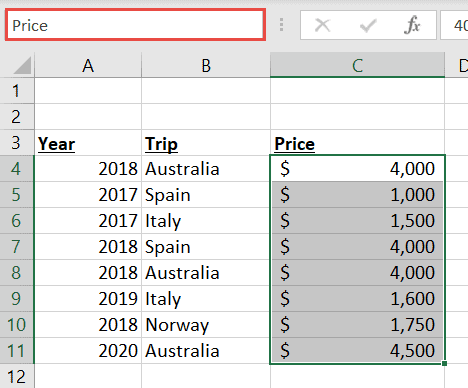
In this example, I want to count the number of trips launched in 2019. To do this, I select the cell range that contains the year I am looking for, and then I specify my criteria, 2019.  

Syntax 

COUNTIF(range, criteria) 

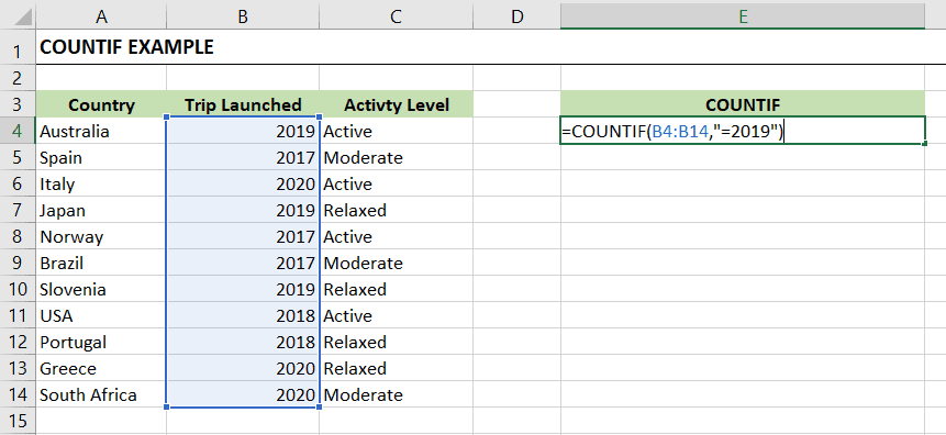
Using COUNTIF, I can search in one range for one piece of criteria.  

The COUNTIFS function 

In this example, I am using COUNTIFS to count the number of trips launched in ‘2019’ that have the activity level of ‘Relaxed’. 

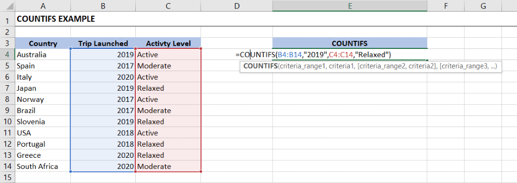
• Type =COUNTIFS into a cell 
• Select the criteria range 1, B4:B14 (the range that contains what you are looking for) 
• Type comma 
• Enter “2019” in quote marks as the criteria 
• Type comma 
• Select the criteria range 2, C4:C14 
• Type comma 
• Enter “Relaxed” in quote marks as the criteria2 
• Press Enter 

The result is 2.  

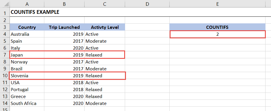
You can specify up to 127 range/criteria pairings in your formulas.  

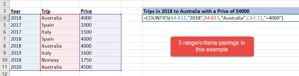
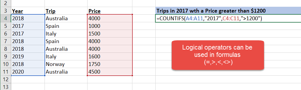
Logical operators can also be used.  

In this example, I am using the greater than (>) logical operator to count the number of trips in 2017 with a price higher than $1200.  

Also Read: 

How To Protect Cells In Excel Workbooks-the Easiest Way

Create An Excel Dashboard In 5 Minutes – The Best Guide

Dynamic Dropdown Lists In Excel – Top Data Validation Guide

Using Named Ranges in Excel COUNTIFS 

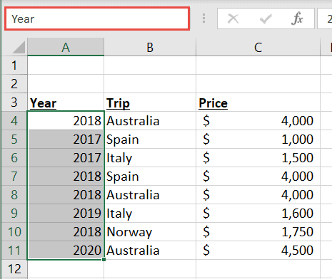
It’s good to get into the habit of naming cell ranges. When you name a range, it gives meaning and helps others understand what cells you are referring to in formulas.  

Naming a Range 

• Select the cell range you wish to name 
• In the Name box above, type in a meaningful name for the range 
• Press Enter 

These named ranges can now be used in the COUNTIFS formula instead of the cell ranges.  

Excel COUNTIFS – Let’s Roundup

The key takeaway of this guide is that the Excel COUNTIFS function is a valuable addition to the list of Excel functions, as it allows us to count based on multiple criteria at once.

 If you have any doubts related to COUNTIFS or other Excel functions, you can ask them in the comments below.  If you want more quality information on advanced features in Excel, check out our Excel courses. 

FAQs

Like what you see? Check out these links for more COUNTIFS examples and if you are feeling brave, why not try using COUNTIFS with a dynamic criteria range.  

Other Excel classes you might like:

• Introduction to Power Pivot & Power Query in Excel
• What-If Analysis in Excel
• Designing Better Spreadsheets in Excel
• How to Use the SUMIF and SUMIFS Function in Microsoft Excel

For more Free Excel tutorials from Simon Sez IT. Take a look at our Excel Resource Center.

To learn Excel with Simon Sez IT. Take a look at the Excel courses we have available.