
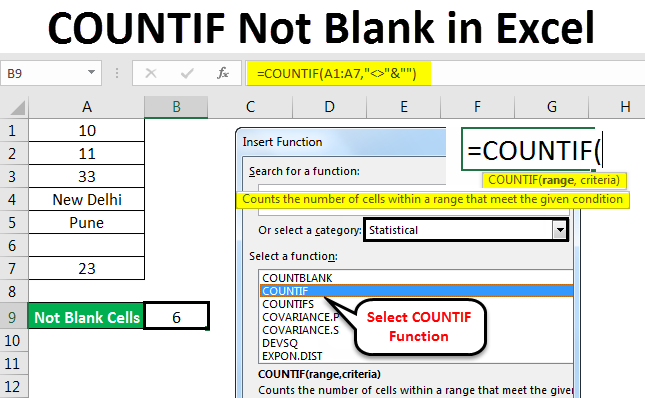
COUNTIF Not Blank Function
The COUNTIF not blank function counts non-blank cells within a range. The universal formula is “COUNTIF(range,”<>”&””)” or “COUNTIF(range,”<>”)”. This formula works with numbers, text, and date values. It also works with the logical operators like “<,” “>,” “=,” and so on.
Note: Alternatively, the COUNTA functionThe COUNTA function is an inbuilt statistical excel function that counts the number of non-blank cells (not empty) in a cell range or the cell reference. For example, cells A1 and A3 contain values but, cell A2 is empty. The formula “=COUNTA(A1,A2,A3)” returns 2.
read more can be used to count the non-blank cells.
Table of contents
- COUNTIF Not Blank Function
- How to Use COUNTIF Non-Blank Function?
- #1–Numerical Values
- #2–Text Values
- #3–Date Values
- The Characteristics of COUNTIF Not Blank Function
- Frequently Asked Questions
- Recommended Articles
- How to Use COUNTIF Non-Blank Function?
How to Use COUNTIF Non-Blank Function?
#1–Numerical Values
The steps to count non-empty cells with the help of the COUNTIF function are listed as follows:
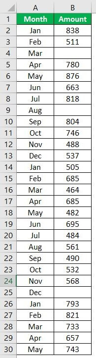
- In Excel, enter the following data containing both, the data cells and the empty cells.

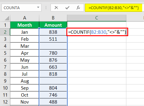
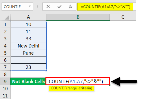
- Enter the following formula to count the data cells.
“=COUNTIF(range,”<>”&””)”
In the range argument, type B2:B30. Alternatively, select the range B2:B30 in the formula, as shown in the following image.

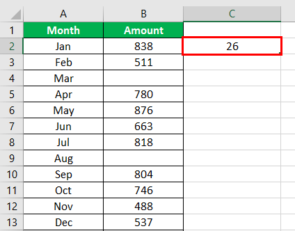
- Press the “Enter” key. The number of non-blank cells in the range B2:B30 appear in cell C2. The output is 26, as shown in the succeeding image.
This implies that there are 26 cells in the given range that contain a data value. This data can be a number, text, or any other value.

#2–Text Values
The steps to count non-empty cells within text values are listed as follows:
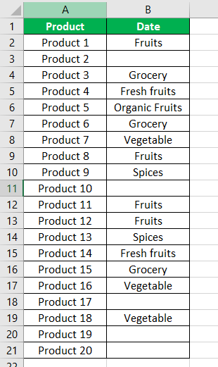
- Step 1: In Excel, enter the data as shown in the following image.
- Step 2: Select the range within which data needs to be checked for non-blank values. Enter the formula shown in the succeeding image.
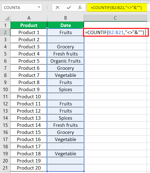
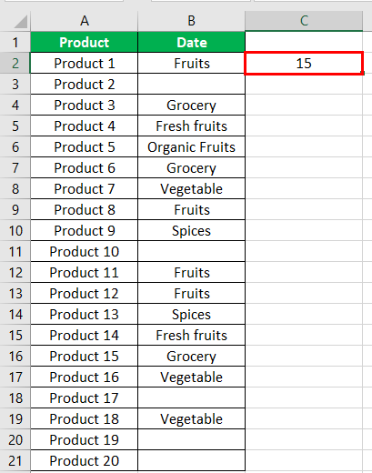
- Step 3: Press the “Enter” key. The number of non-blank cells in the range B2:B21 appear in cell C2. The output is 15, as shown in the succeeding image.
Hence, the COUNTIF not blank formula works with text values.
#3–Date Values
The steps to count non-empty cells, when the data consists of dates, are listed as follows:
- Step 1: In Excel, enter the data as shown in the following image. Select the range whose data needs to be checked for non-blank values. Enter the following formula.
“=COUNTIF(B2:B21,”<>”&””)”
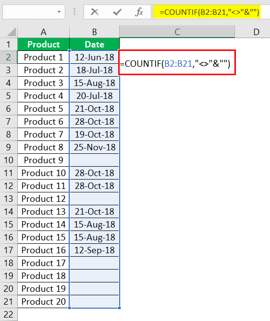
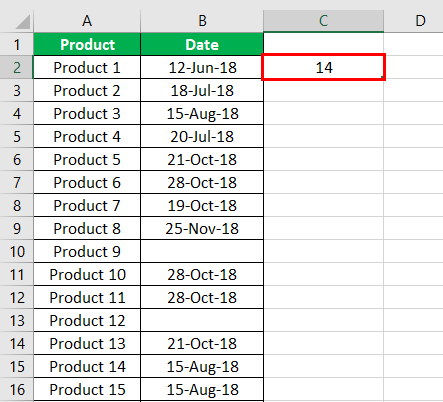
- Step 2: Press the “Enter” key. The number of non-blank cells in the range B2:B21 appear in cell C2. The output is 14, as shown in the succeeding image.
Hence, the COUNTIF not blank formula works with data that consists of date values.
The Characteristics of COUNTIF Not Blank Function
- It is case insensitive, implying that the output remains the same irrespective of whether the formula is entered in uppercase or lowercase.
- It works for data that consists of numbers, text, and date values.
- It works with greater than (>) and less than (<) operators.
- It is difficult to use the formula with long strings.
- The criteria (condition) must be specified within a pair of inverted commas to avoid errors.
Frequently Asked Questions
How is the COUNTIF formula used to count blanks?
The universal formula for counting blanks is stated as follows:
“COUNTIF(range,””)”
This formula works with all types of data values.
Note: Alternatively, the COUNTBLANK function can be used to count blank cells.
How does the COUNTIF function count the duplicate values?
The formula for counting the duplicate value is given as follows:
“COUNTIF(range,“duplicate value”)”
The “range” represents the range within which the duplicate values are to be counted. The “duplicate value” is the exact data value that is to be counted.
For example, to count the number of times the text “fruits” appears in the range A2:A10, we use “=COUNTIF(A2:A10,“fruits”).”
- The COUNTIF not blank function counts the non-blank cells within a given range.
- The generic formula of the COUNTIF not blank function is stated as–“COUNTIF (range,“<>”&””).”
- The criteria (condition) must be specified within a pair of inverted commas to avoid errors.
- The COUNTIF functionThe COUNTIF function in Excel counts the number of cells within a range based on pre-defined criteria. It is used to count cells that include dates, numbers, or text. For example, COUNTIF(A1:A10,”Trump”) will count the number of cells within the range A1:A10 that contain the text “Trump”
read more works for data that consists of numbers, text, and date values. - The COUNTIF formula gives the same output irrespective of whether the formula is entered in uppercase or lowercase.
Recommended Articles
This has been a guide to Excel COUNTIF not blank. Here we discuss how to use the COUNTIF function to count non-blank cells along with practical examples and a downloadable Excel template. You may learn more about Excel from the following articles –
- Not Equal in VBA
- COUNTIF with Multiple Criteria
- VLOOKUP Errors
- Use Not Equal to in Excel
- XML in Excel
In this example, the goal is to count cells in a range that are not blank (i.e. not empty). There are several ways to go about this task, depending on your needs. The article below explains different approaches.
COUNTA function
While the COUNT function only counts numbers, the COUNTA function counts both numbers and text. This means you can use COUNTA as a simple way to count cells that are not blank. In the example shown, the formula in F6 uses COUNTA like this:
=COUNTA(C5:C16) // returns 9
Since there are nine cells in the range C5:C16 that contain values, COUNTA returns 9. COUNTA is fully automatic, so there is nothing to configure.
COUNTIFS function
You can also use the COUNTIFS function to count cells that are not blank like this:
=COUNTIFS(C5:C16,"<>") // returns 9
The «<>» operator means «not equal to» in Excel, so this formula literally means count cells not equal to nothing. Because COUNTIFS can handle multiple criteria, we can easily extend this formula to count cells that are not empty in Group «A» like this:
=COUNTIFS(B5:B16,"A",C5:C16,"<>") // returns 4
The first range/criteria pair selects cells that are in Group A only. The second range/criteria pair selects cells that are not empty. The result from COUNTIFS is 4, since there are 4 cells in Group A that are not empty. You can swap the order of the range/criteria pairs with the same result.
See also: 50 examples of formula criteria.
SUMPRODUCT function
One problem with COUNTA and COUNTIFS is that they will also count empty strings («») returned by formulas as not blank, even though these cells are intended to be blank. For example, if A1 contains 21, this formula in B1 will return an empty string:
=IF(A1>30,"Overdue","")However, COUNTA and COUNTIFS will still count B1 as not empty. If you run into this problem, you can use the SUMPRODUCT function to count cells that are not blank like this:
=SUMPRODUCT(--(C5:C16<>""))

The expression C5:C16<>»» returns an array that contains 12 TRUE and FALSE values, and the double negative (—) converts the TRUE and FALSE values to 1s and 0s:
=SUMPRODUCT({1;1;0;1;1;0;1;1;1;0;1;1}) // returns 9
The result is 9 as before. But this formula will also ignore cells that contain formulas that return empty strings.
You can easily extend the logic used in SUMPRODUCT with other functions as needed. For example, the variant below uses the LEN function to count cells that have a length greater than zero:
=SUMPRODUCT(--(LEN(C5:C16)>0)) // returns 9
You can extend the formula to count cells that are not blank in Group A like this:
=SUMPRODUCT((LEN(C5:C16)>0)*(B5:B16="A"))
This is an example of using Boolean algebra in a formula. The double negative is no longer needed in this case because the math operation of multiplying the two arrays together automatically converts the TRUE and FALSE values to 1s and 0s:
=SUMPRODUCT({1;1;0;1;1;0;0;0;0;0;0;0}) // returns 4
The final result is 4, since there are four cells in Group A that are not blank in C5:C16.
Note: one reason the Boolean syntax above is useful is because you can drop the same logical expressions into a newer function like the FILTER function to extract cells that meet the same criteria. The SUMPRODUCT function is more versatile than RACON functions like COUNTIFS, SUMIFS, etc. and you will often see it used in formulas that solve tricky problems. You can read more about SUMPRODUCT here.
COUNTIF function
Use COUNTIF, one of the statistical functions, to count the number of cells that meet a criterion; for example, to count the number of times a particular city appears in a customer list.
In its simplest form, COUNTIF says:
-
=COUNTIF(Where do you want to look?, What do you want to look for?)
For example:
-
=COUNTIF(A2:A5,»London»)
-
=COUNTIF(A2:A5,A4)

COUNTIF(range, criteria)
|
Argument name |
Description |
|---|---|
|
range (required) |
The group of cells you want to count. Range can contain numbers, arrays, a named range, or references that contain numbers. Blank and text values are ignored. Learn how to select ranges in a worksheet. |
|
criteria (required) |
A number, expression, cell reference, or text string that determines which cells will be counted. For example, you can use a number like 32, a comparison like «>32», a cell like B4, or a word like «apples». COUNTIF uses only a single criteria. Use COUNTIFS if you want to use multiple criteria. |
Examples
To use these examples in Excel, copy the data in the table below, and paste it in cell A1 of a new worksheet.
|
Data |
Data |
|---|---|
|
apples |
32 |
|
oranges |
54 |
|
peaches |
75 |
|
apples |
86 |
|
Formula |
Description |
|
=COUNTIF(A2:A5,»apples») |
Counts the number of cells with apples in cells A2 through A5. The result is 2. |
|
=COUNTIF(A2:A5,A4) |
Counts the number of cells with peaches (the value in A4) in cells A2 through A5. The result is 1. |
|
=COUNTIF(A2:A5,A2)+COUNTIF(A2:A5,A3) |
Counts the number of apples (the value in A2), and oranges (the value in A3) in cells A2 through A5. The result is 3. This formula uses COUNTIF twice to specify multiple criteria, one criteria per expression. You could also use the COUNTIFS function. |
|
=COUNTIF(B2:B5,»>55″) |
Counts the number of cells with a value greater than 55 in cells B2 through B5. The result is 2. |
|
=COUNTIF(B2:B5,»<>»&B4) |
Counts the number of cells with a value not equal to 75 in cells B2 through B5. The ampersand (&) merges the comparison operator for not equal to (<>) and the value in B4 to read =COUNTIF(B2:B5,»<>75″). The result is 3. |
|
=COUNTIF(B2:B5,»>=32″)-COUNTIF(B2:B5,»<=85″) |
Counts the number of cells with a value greater than (>) or equal to (=) 32 and less than (<) or equal to (=) 85 in cells B2 through B5. The result is 1. |
|
=COUNTIF(A2:A5,»*») |
Counts the number of cells containing any text in cells A2 through A5. The asterisk (*) is used as the wildcard character to match any character. The result is 4. |
|
=COUNTIF(A2:A5,»?????es») |
Counts the number of cells that have exactly 7 characters, and end with the letters «es» in cells A2 through A5. The question mark (?) is used as the wildcard character to match individual characters. The result is 2. |
Common Problems
|
Problem |
What went wrong |
|---|---|
|
Wrong value returned for long strings. |
The COUNTIF function returns incorrect results when you use it to match strings longer than 255 characters. To match strings longer than 255 characters, use the CONCATENATE function or the concatenate operator &. For example, =COUNTIF(A2:A5,»long string»&»another long string»). |
|
No value returned when you expect a value. |
Be sure to enclose the criteria argument in quotes. |
|
A COUNTIF formula receives a #VALUE! error when referring to another worksheet. |
This error occurs when the formula that contains the function refers to cells or a range in a closed workbook and the cells are calculated. For this feature to work, the other workbook must be open. |
Best practices
|
Do this |
Why |
|---|---|
|
Be aware that COUNTIF ignores upper and lower case in text strings. |
|
|
Use wildcard characters. |
Wildcard characters —the question mark (?) and asterisk (*)—can be used in criteria. A question mark matches any single character. An asterisk matches any sequence of characters. If you want to find an actual question mark or asterisk, type a tilde (~) in front of the character. For example, =COUNTIF(A2:A5,»apple?») will count all instances of «apple» with a last letter that could vary. |
|
Make sure your data doesn’t contain erroneous characters. |
When counting text values, make sure the data doesn’t contain leading spaces, trailing spaces, inconsistent use of straight and curly quotation marks, or nonprinting characters. In these cases, COUNTIF might return an unexpected value. Try using the CLEAN function or the TRIM function. |
|
For convenience, use named ranges |
COUNTIF supports named ranges in a formula (such as =COUNTIF(fruit,»>=32″)-COUNTIF(fruit,»>85″). The named range can be in the current worksheet, another worksheet in the same workbook, or from a different workbook. To reference from another workbook, that second workbook also must be open. |
Note: The COUNTIF function will not count cells based on cell background or font color. However, Excel supports User-Defined Functions (UDFs) using the Microsoft Visual Basic for Applications (VBA) operations on cells based on background or font color. Here is an example of how you can Count the number of cells with specific cell color by using VBA.
Need more help?
You can always ask an expert in the Excel Tech Community or get support in the Answers community.

See also
COUNTIFS function
IF function
COUNTA function
Overview of formulas in Excel
IFS function
SUMIF function
Need more help?
Want more options?
Explore subscription benefits, browse training courses, learn how to secure your device, and more.
Communities help you ask and answer questions, give feedback, and hear from experts with rich knowledge.
Author: Oscar Cronquist Article last updated on January 08, 2023
![]()
The COUNTIF function is very capable of counting non-empty values, I will show you how in this article. Excel can also highlight empty cells using Conditional formatting.
I will discuss and demonstrate the limitations of using the COUNTIF function and other equivalent functions that you also can use.
What’s on this page
- Count not blank cells — COUNTIF function
- Count not blank cells — COUNTA function
- COUNTIF and COUNTA function return unexpected results
- Count not blank cells — SUMPRODUCT function
- Get Excel *.xlsx file
1. Count not blank cells — COUNTIF function
![]()
Column B above has a few blank cells, they are in fact completely empty.
Formula in cell D3:
=COUNTIF(B3:B13,»<>»)
The first argument in the COUNTIF function is the cell range where you want to count matching cells to a specific value, the second argument is the value you want to count.
COUNTIF(range, criteria)
In this case, it is «<>» meaning not equal to and then nothing, so the COUNTIF function counts the number of cells that are not equal to nothing. In other words, cells that are not empty.

Back to top
2. Count not blank cells — COUNTA function
![]()
The COUNTA function is even easier to use, you don’t need to enter more than the cell range in one argument. The COUNTA function is designed to count non-empty cells.
COUNTA(value1, [value2], …)
Formula in cell D4:
=COUNTA(B3:B13)
Back to top
3. COUNTIF and COUNTA function return unexpected results
![]()
There are, however, situations where the COUNTIF and COUNTA function return unexpected results if you are not aware of how they work.
There are blank cells in column C, shown in the picture above, that look empty but they are not. Column D shows what they actually contain and column E shows the character length of the content.
Cell C5 and C9 contain a formula that returns a blank, both the COUNTIF and the COUNTA function count those cells as non-empty.
Cell C8 has two space characters and cell C12 has one space character, column E reveals their existence by counting character length. The COUNTIF and the COUNTA function count those cells as non-empty as well.
Back to top
4. Count not blank cells — SUMPRODUCT function
![]()
The following formula counts all non-empty values in cell range C3:C13 except formulas that return nothing. It checks if the values in cell range C3:C13 are not equal to nothing.
Formula in cell B16:
=SUMPRODUCT((C3:C13<>»»)*1)
Back to top
4.1 Explaining formula in cell B16
Step 1 — Check if cells are not empty
In this case, the logical expression counts cells that contain space characters but not formulas that return nothing.
The less than and the greater than characters are logical operators, the result are always boolean values.
C3:C13<>»»
returns
{TRUE; TRUE; FALSE; TRUE; TRUE; TRUE; FALSE; TRUE; TRUE; TRUE; TRUE}
Step 2 — Convert boolean values
The SUMPRODUCT function can’t sum boolean values, we need to multiply with one to create an array containing 0’s (zero) and 1’s.
They are their numerical equivalents:
True = 1
FALSE = 0 (zero)
(C3:C13<>»»)*1
becomes
{TRUE; TRUE; FALSE; TRUE; TRUE; TRUE; FALSE; TRUE; TRUE; TRUE; TRUE}*1
and returns
{1; 1; 0; 1; 1; 1; 0; 1; 1; 1; 1}
Step 3 — Sum numbers
Why use the SUMPRODUCT function and not the SUM function? The SUMPRODUCT function can perform calculations in the arguments without the need to enter the formula as an array formula.
Array formulas are great but if possible avoid as much as you can. Excel 365 users don’t have this problem, dynamic array formulas are entered as regular formulas.
SUMPRODUCT((C3:C13<>»»)*1)
becomes
SUMPRODUCT({1; 1; 0; 1; 1; 1; 0; 1; 1; 1; 1})
and returns 9 in cell B16.
Back to top
5. Regard formulas that return nothing to be blank and space characters to also be blank
![]()
The formula above in cell C16 counts only non-empty values, it considers formulas that return nothing to be blank and space characters to also be blank. This is made possible by the TRIM function that removes leading and ending space characters.
=SUMPRODUCT((TRIM(C3:C13)<>»»)*1)
Back to top
5.1 Explaining formula in cell B16
Step 1 — Remove space characters
TRIM(C3:C13)
returns
{«Green»; «Blue»; «»; «Red»; «Cyan»; «»; «»; «Yellow»; «Orange»; «»; «Brown»}
Step 2 — Identify not blank cells
TRIM(C3:C13)<>»»
becomes
{«Green»; «Blue»; «»; «Red»; «Cyan»; «»; «»; «Yellow»; «Orange»; «»; «Brown»}<>»»
and returns
{TRUE; TRUE; FALSE; TRUE; TRUE; FALSE; FALSE; TRUE; TRUE; FALSE; TRUE}
Step 3 — Multiply with 1
TRIM(C3:C13)<>»»)*1
becomes
{TRUE; TRUE; FALSE; TRUE; TRUE; FALSE; FALSE; TRUE; TRUE; FALSE; TRUE}*1
and returns
{1; 1; 0; 1; 1; 0; 0; 1; 1; 0; 1}
Step 4 — Sum numbers in array
SUMPRODUCT((TRIM(C3:C13)<>»»)*1)
becomes
SUMPRODUCT({1; 1; 0; 1; 1; 0; 0; 1; 1; 0; 1})
and returns 7.
Back to top
Latest updated articles.
More than 300 Excel functions with detailed information including syntax, arguments, return values, and examples for most of the functions used in Excel formulas.
More than 1300 formulas organized in subcategories.
Excel Tables simplifies your work with data, adding or removing data, filtering, totals, sorting, enhance readability using cell formatting, cell references, formulas, and more.
Allows you to filter data based on selected value , a given text, or other criteria. It also lets you filter existing data or move filtered values to a new location.
Lets you control what a user can type into a cell. It allows you to specifiy conditions and show a custom message if entered data is not valid.
Lets the user work more efficiently by showing a list that the user can select a value from. This lets you control what is shown in the list and is faster than typing into a cell.
Lets you name one or more cells, this makes it easier to find cells using the Name box, read and understand formulas containing names instead of cell references.
The Excel Solver is a free add-in that uses objective cells, constraints based on formulas on a worksheet to perform what-if analysis and other decision problems like permutations and combinations.
An Excel feature that lets you visualize data in a graph.
Format cells or cell values based a condition or criteria, there a multiple built-in Conditional Formatting tools you can use or use a custom-made conditional formatting formula.
Lets you quickly summarize vast amounts of data in a very user-friendly way. This powerful Excel feature lets you then analyze, organize and categorize important data efficiently.
VBA stands for Visual Basic for Applications and is a computer programming language developed by Microsoft, it allows you to automate time-consuming tasks and create custom functions.
A program or subroutine built in VBA that anyone can create. Use the macro-recorder to quickly create your own VBA macros.
UDF stands for User Defined Functions and is custom built functions anyone can create.
A list of all published articles.
![]()
- COUNTIF не пустой в Excel
![]()
COUNTIF Excel не пустой (оглавление)
- COUNTIF не пустой в Excel
- Синтаксис COUNTIF не пустой в Excel
- Как использовать COUNTIF Not Blank в Excel?
COUNTIF не пустой в Excel
Функция COUNTIF Not Blank используется для подсчета любого определенного числа / диапазона текста любого столбца без учета какой-либо пустой ячейки. Это становится возможным только при использовании функции COUNTIF, которая следует заданным критериям для получения желаемого результата.
Синтаксис COUNTIF не пустой в Excel
![]()
COUNTIF (Диапазон, Критерии)
Синтаксис для функции COUNTIF включает в себя 2 параметра:
Диапазон = Это диапазон, который нам нужно выбрать, из которого мы будем получать счет.
Критерии = Критерии должны быть любым точным словом или числом, которое мы должны посчитать.
Возвращаемое значение COUNTIF в Excel является положительным числом. Значение может быть нулевым или ненулевым.
Как пользоваться?
Использовать Excel Countif Not Blank очень просто. Здесь мы увидим, как использовать функцию COUNTIF, чтобы найти, сколько ячеек не являются пустыми в листе Excel. Давайте разберемся, как работает функция COUNTIF в Excel, на следующих примерах.
Вы можете скачать этот шаблон Excel COUNTIF Not Blank здесь — Шаблон Excel COUNTIF Not Blank
COUNTIF не пуст в Excel — пример № 1
У нас есть небольшие данные произвольного текста и чисел в столбце. И в этом столбце также есть пустая ячейка. Теперь для большого количества данных становится очень трудно сосчитать ячейку без пустых ячеек. Итак, мы применим функцию COUNTIF с комбинацией критериев, которая позволяет формуле пренебрегать пробелом и дает общее количество ячеек, которое имеет некоторое значение.
![]()
Как мы видим на скриншоте выше, в столбце A у нас есть данные, начиная с A2 до A7, и между ними в A6 находится пустая ячейка. Теперь, чтобы подсчитать общее количество ячеек, но не пустых, используйте COUNTIF. Для этого перейдите в любую ячейку, где вы хотите увидеть вывод, и нажмите fx (вкладка для вставки функций в Excel), как показано ниже.
![]()
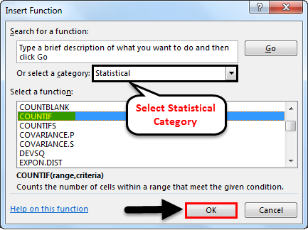
Эта вкладка FX доступна чуть ниже строки меню . Как только мы щелкнем по нему, мы получим поле Вставить функцию, в котором будут все встроенные функции, предоставляемые Microsoft в ячейке. Найдите функцию COUNTIF, прокрутив ее вверх и вниз, а затем нажмите Ok, как показано на скриншоте ниже.
![]()
Как мы видим в приведенном выше поле «Вставка функции», есть вкладка « Выбор категории», в которой есть все категории для определенных функций. Отсюда мы можем перемещаться, чтобы выбрать все параметры, как показано на скриншоте выше, или мы можем выбрать Статистическую категорию, где мы найдем функцию COUNTIF, как показано на скриншоте ниже. А затем нажмите ОК.
![]()
Как только мы нажмем Ok, появится другое окно с аргументами функций, в котором нам нужно будет определить диапазон и критерии. Здесь мы выбрали диапазон от A2 до A7 и критерий как «» & », что означает, что ячейка, содержащая значение, большее и меньшее, чем любой пробел, должна учитываться. И нажмите ОК.
![]()
Критерии могут быть любыми, но для непустой ячейки нам нужно выбрать ячейку с любым значением, большим или меньшим, чем пустое. Для этого мы использовали «&»
Если критерии, которые мы определили, верны, то в окне «Аргументы функции» будут отображаться выходные данные в поле, как показано выше в нижней левой части окна. Как это показывает результат нашего определенного диапазона и критериев как 6.
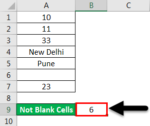
Также на скриншоте ниже мы получили количество ячеек, которые не являются пустыми, как 6 . Поскольку ячейка A6 пуста, COUNTIF пренебрег этой пустой ячейкой и дал результат оставшегося числа ячеек, которое имеет некоторое значение (число или текст).
![]()
COUNTIF не пуст в Excel — пример № 2
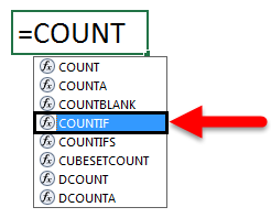
Существует другой метод использования COUNTIF, не пустой, который подсчитывает все выбранные ячейки, но не пустые, путем непосредственного редактирования ячейки. Для этого перейдите в режим редактирования любой ячейки и нажмите знак равенства «=», что активирует все встроенные функции Excel. Там введите COUNTIF и выберите его, как показано на скриншоте ниже.
Нажатие «=» (знак равенства) в любой ячейке включает все функции, доступные в Excel. И даже если мы введем отдельные слова (скажем, «Количество»), как показано на скриншоте ниже, это даст все возможные функции, доступные для использования. Оттуда также мы можем выбрать функцию согласно нашему требованию.
![]()
![]()
Как вы можете видеть на скриншоте выше, функция COUNTIF имеет диапазон и критерии, которые должны быть назначены, что также было в предыдущем примере. Поэтому мы назначим тот же диапазон, что и для A2, и A7, а критерии — для «» & », как показано ниже.
![]()
И нажмите клавишу ввода. Мы получим количество ячеек, значение которого равно «6», но мы выбрали всего 7 ячеек, включая ячейку A6, которая не заполнена. Здесь также функции COUNTIF подсчитывают общее количество ячеек, которые не являются пустыми.
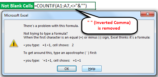
Но если мы введем неправильные критерии, мы можем получить сообщение об ошибке, которое объяснит возникшую проблему, как показано на скриншоте ниже. Здесь для тестирования мы удалили «» (кавычки) из критериев и получили ошибку.
![]()
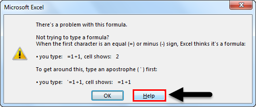
Если мы не знаем, как устранить ошибку, то мы можем нажать кнопку « Справка», показанную на снимке экрана ниже, что приведет нас непосредственно к окну справки Microsoft Excel, которое поможет правильно настроить аргументы функции.
![]()
Замечания:
- «« (Перевернутая запятая) в функции Excel используется, когда есть какой-либо текст или необходимо захватить пустую ячейку. Вот текст и «» вместе используются для захвата ячейки, которая имеет какое-либо значение, но не является пустой.
- Используя « &» в формуле, мы можем добавить больше критериев в соответствии с нашим требованием.
Плюсы Excel COUNTIF не пустые в Excel
- Для больших наборов данных, где применение фильтра занимает так много времени, использование функции Excel Countif Not Blank полезно и экономит время, так как подсчет ячеек не пустой.
- Это дает мгновенный и точный результат.
- COUNTIF формула полностью автоматическая, она проста и удобна в использовании.
- Это очень полезно в бухгалтерской работе.
То, что нужно запомнить
- Всегда проверяйте данные, если это перенесенные выходные данные из другого источника. Есть вероятность того, что данные могут содержать пустые ячейки со скрытыми значениями. В этом случае отфильтруйте пустую ячейку и удалите значения ячейки, чтобы избежать неправильного вывода.
- Всегда показывайте лист или столбец, чтобы получить точный результат.
Рекомендуемые статьи
Это было руководство к COUNTIF, а не пустым в Excel. Здесь мы обсудим, как использовать функцию COUNTIF для подсчета не пустых ячеек в Excel, а также с практическими иллюстрациями и загружаемым шаблоном Excel. Вы также можете просмотреть наши другие предлагаемые статьи —
- Как использовать функцию COUNTIF Excel?
- Руководство по COUNTIF с несколькими критериями
- Не равно функции в Excel
- Как считать строки в Excel?
This is going to be a super simple post, here our aim is to find the number of cells that contain data, cells that are blank or empty should be excluded. The task is quite simple but the question becomes ‘how to do it?’. You know you want Excel to count a certain type of cells for you but if you find yourself wondering what to put in your sheets to get that count, you’re about to find out.
This tutorial will walk you through the usage of functions to count non-blank cells and at the end, we will also see a few functions to selectively count only the blank cells. So, without further ado, let’s jump right in.
 1")
Counting Cells That Are Not Blank
Here we are going to talk about three Excel functions that can help us to count non-blank cells from a range.
Using COUNTIF Function
The COUNTIF function counts the number of cells within a range that meet the given criteria. COUNTIF asks for the range from which it needs to count and the criteria according to which it needs to count. To count all the non-blank cells with COUNTIF we can make use of the following formula:
=COUNTIF(range,"<>")
Let’s try to understand this with an example. So, we have a dataset as shown below:
 2")
From this list of product discounts, we will aim to find how many products are discounted. In Excel’s terminology, this means – we are finding out how many non-blank cells there are in column D (the non-blank cells represent the discounts on products and the blank cells represent products with no discount).
We can easily accomplish this using the following COUNTIF formula:
=COUNTIF(D3:D14,"<>")
And our final result looks something like this.
 3")
Here, the formula has been fed with the range of column D (D3:D14). The criteria for searching column D is «<>» which is the indicator for non-blank cells («» for blank cells).
The COUNTIF function has counted 8 non-blank cells as the result. This tells us that in our dataset, there are 8 products on discount.
The COUNTIF function can be used for only one condition. For multiple conditions (e.g., non-blank cells and discount more than 20%), we can use the COUNTIFS function.
The next function we will use to count if not blank cells are present in a range is the COUNTA function.
Using COUNTA Function
By its nature, the COUNTA function counts the cells in a range that are not empty. It is a single argument function (in its simplest form) requiring just the range from which to count non-blank cells.
We will use it in our last example and simply add our range D3:D14 to the COUNTA function in this way:
=COUNTA(D3:D14)
We have the same results as the COUNTIF function i.e., 8 non-blank cells, with fewer arguments.
 4")
For the sole purpose of counting non-blank cells, the COUNTA function offers an easy, straightforward solution.
However, the COUNTA and COUNTIF functions will also count cells with space characters and formulas that return an empty string. This means that the functions will count cells that look blank but are not essentially blank.
Why is that a problem?
Technically, a space character or a formula that returns an empty string is very different from a blank cell. Although they look similar but technically they are two different things.
But since our purpose here is to count non-blank cells, so we might want the cells that appear blank to be counted as blank cells (technically, even though they are not blank). To accomplish this instead of using the COUNTIF or COUNTA functions it is better to use a SUMPRODUCT function. And this is what we are going to see in the next section.
Tip: If you are adamant about using the COUNTIF or COUNTA function for counting non-blank cells, another way around it would be to filter the data and get rid of the cells with hidden values. This will refine the results without the inclusion of faux blank cells. For now, we will move onto the SUMPRODUCT function.
Using SUMPRODUCT Function
The SUMPRODUCT returns the sum of the products of the supplied ranges or arrays. To count non-blank cells using SUMPRODUCT function we can use the below formula:
=SUMPRODUCT(--(C2:C13<>""))
Let’s try to understand the formula first and then we can compare it with the COUNTIF and COUNTA functions.
In the above formula, first of all, we are checking if the values in the range C2:C13 are equal to an empty string (nothing). This returns an array of boolean values like this –
=SUMPRODUCT(--({TRUE, TRUE, TRUE, FALSE, TRUE, TRUE, TRUE, TRUE, FALSE, TRUE, TRUE, TRUE}))
Now, since the SUMPRODUCT function cannot sum boolean values we are converting them to 0’s and 1’s by using the double-negatives. So, the formula gets further simplified to something like this –
=SUMPRODUCT({1, 1, 1, 0, 1, 1, 1, 1, 0, 1, 1, 1})
The SUMPRODUCT function adds all these 1’s and 0’s and returns the final result.
An important thing worth noting here is that the above formula does not treat space character as an empty string (nothing) so it will still be counted as a non-blank cell. To count them as blanks we can make use of the TRIM function and the final formula would look like this –
=SUMPRODUCT(--(TRIM(C2:C13)<>""))
Pro Tip: Instead of using the double negatives to convert boolean values to 1’s and 0’s we can also either add 0 to them or multiply them by 1 and our final result would still be the same.
Now, Let’s have the COUNTIF, COUNTA, and SUMPRODUCT functions side by side and analyze them:
 5")
What we can see from the serial numbering, is that there are 12 rows in our dataset. C5 is a blank cell that is correctly interpreted as blank cells by COUNTIF and COUNTA. It appears that there are 2 more blank cells (C8 containing a space character and C10 containing a formula that returns an empty string i.e., =»») in the range which means that there are 9 non-blank cells.
While the COUNTIF and COUNTA functions have treated C5 as a blank cell but they treat the other two C8 and C10 as non-blank cells and thus return 11 as the count.
On the other hand, the SUMPRODUCT based formula correctly identifies all such cells and hence returns 9 as the count of non-blank cells.
Recommended Reading: Counting Unique Values In Excel
Counting Blank Cells
Now is the turn for counting blank cells. We have ahead 2 very simple ways of counting empty cells with help of the COUNTBLANK and the COUNTIF function.
Using COUNTBLANK Function
The COUNTBLANK function, pretty self-explanatory, counts the number of empty/blank cells in a specified range. We will use the function plainly to get our results:
=COUNTBLANK(D3:D14)
 6")
We have inserted the range D3:D14 in the formula to see how many blank cells there are in column D which will tell us the number of products with no discount. The outcome of the COUNTBLANK function is «4» blank cells.
Using COUNTIF Function
As explained above, the COUNTIF function can be used for counting both, blank and non-blank cells. Now we will see how to use COUNTIF for counting blank cells.
To count blank cells the COUNTIF function can be used as:
=COUNTIF(D3:D14,"")
 7")
In the formula, which is made up of the range and criteria, we have swapped the criteria for counting non-blank cells (i.e., «<>») with the criteria for counting blank cells (i.e., «»). With the range specified as D3:D14, the COUNTIF function returns «4» blank cells as the result, indicating 4 undiscounted products.
At the end of this tutorial, we hope you won’t feel blank when trying to count if not blank and blank cells. We’re following up with more how-to’s as you read!
Excel COUNTIF Not Blank (Table of Contents)
- COUNTIF Not Blank in Excel
- The syntax for COUNTIF Not Blank in Excel
- How to use COUNTIF Not Blank in Excel?
COUNTIF Not Blank in Excel
COUNTIF Not Blank function is used for counting of any defined number/text range of any column without considering any blank cell. This becomes possible only by using the COUNTIF function, which follows the defined criteria to get the desired output.
Syntax for COUNTIF Not Blank in Excel
COUNTIF(Range, Criteria)
Syntax for COUNTIF Function includes 2 parameters which are as follows:
Range = The range we need to select from where we will get the count.
Criteria = Criteria should be any exact word or number we need to count.
The return value of COUNTIF in Excel is a positive number. The value can be zero or non-zero.
How to Use?
Using Excel Countif Not Blank is very easy. Here we will see How to use COUNTIF Function to find how many cells are not blank in the Excel sheet. Let’s understand the working of the COUNTIF Function in Excel through some examples below.
You can download this Excel COUNTIF Not Blank Template here – Excel COUNTIF Not Blank Template
COUNTIF Not Blank in Excel – Example #1
We have small data of some random text and numbers in a column. And this column has a blank cell as well. It becomes very difficult to count the cell without blank cells for a large amount of data. So, we will apply the COUNTIF function with the combination of criteria that allow the formula to neglect the blank and give a total number of cells with some value.
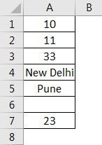
As we can see in the above screenshot, column A has data from A2 to A7, and it has a blank cell in between at A6. Now to count the total cells but not blank, use COUNTIF. For that, go to any cell where you want to see the output and click on fx (a tab to insert functions in excel), as shown below.
![]()
This fx tab is available just below the Menu bar. Once we click on it, we will get an Insert Function box, which has all the built-in functions provided by Microsoft in a cell. Please search for the COUNTIF function by scrolling it up and down and then clicking Ok, as shown in the below screenshot.
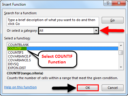
As we can see in the above Insert Function box, there is a tab named Or Select a category, which has all the categories for defined functions in it. From here, we can navigate to select All options, as shown in the above screenshot, or we can select Statistical category, where we will find the COUNTIF function, as shown in the below screenshot. And then click on Ok.
Once we click on Ok, another box will appear for Function Arguments, where we will need to define the Range and Criteria. Here, we have selected the range from A2 to A7 and Criteria as “<>” &,” which means cells containing values greater and lesser than any blank should be counted. And click on Ok.
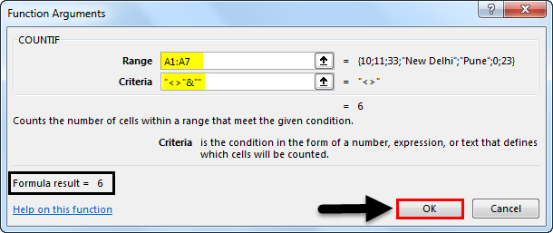
The criteria can be anything, but for a non-blank cell, we need to select a cell with any value greater or lesser than blank. For that, we used “<>” &””
If the criteria we have defined are correct, then the Function Arguments box will show the box’s output as shown above on the bottom left side of the box. It shows the result of our defined range and criteria as 6.
Also, in the below screenshot, we got a count of cells that are not blank as 6. As cell A6 is blank, so COUNTIF has neglected that blank cell and gave the output of the remaining cell count, which has some value (number or text).
COUNTIF Not Blank in Excel – Example #2
There is another method of using COUNTIF, not blank, which counts all selected cells but not blank by directly editing the cell. For this, go to the edit mode of any cell and press the equal “=” sign, enabling all the inbuilt functions of excel. There type COUNTIF and select it, as shown in the below screenshot.
Pressing “=” (Equal sign) in any cell enables all the functions available in Excel. And even if we type selective words (Let’s say “Count”), as shown in the screenshot below, it will give all the possible functions available. From there also, we can select the function as per our requirement.
As you can see in the above screenshot, the COUNTIF function has a range and criteria to be assigned, which was also there in the previous example. So we will assign the same range as A2 to A7 and criteria as “<>” &””, as shown below.
And press Enter key. We will get the count of cells with value, which is “6”, but we selected 7 cells, including cell A6, which is blank. Here also, COUNTIF functions count the total cells that are not blank.
But if we put incorrect criteria, we may get an error message, which will explain the problem, as shown in the screenshot below. Here, we have removed “” (Inverted Commas) from the Criteria and got the error for testing.
If we do not know how to resolve the error, we can click on the Help button, shown in the below screenshot, which will directly take us to the Microsoft Excel Help window, guiding us to make function arguments right.
Note:
- “”(Inverted Comma) in the excel function is used when any text or blank cell needs to be captured. Here <> is the text and “” together are used to capture the cell with any value but is not blank.
- Using “&” in a formula, we can add more criteria per our requirement.
Pros of Excel COUNTIF Not Blank in Excel
- For large sets of data, where applying a filter takes so much time, they’re using Excel Countif Not Blank feature is useful and time-saving for counting cells not blank.
- It gives an instant and exact result.
- The COUNTIF formula is fully automatic; it is easy and instant to use.
- It is very helpful in accounting work.
Things to Remember
- Always check the data if it is migrated output of a different source. There are some chances that the data may contain blank cells with hidden values. In that case, filter the blank cell and delete the cell values to avoid incorrect output.
- Always unhide the sheet or column to get the exact result.
Recommended Articles
This has been a guide to COUNTIF Not Blank in Excel. Here we discuss how to use COUNTIF Function to count Not Blank cells in excel, along with practical illustrations and a downloadable excel template. You can also go through our other suggested articles –
- COUNTIF Excel Function
- COUNTIF with Multiple Criteria
- COUNTIFS in Excel
- COUNTIF Examples in Excel
Excel tables with their functions come in handy to count cells with data, horizontally and vertically. COUNTIF is the common function for counting cells with one and several conditions. So let’s look into this further to understand all the details and distinctions.
Meaning of COUNTIF Excel
COUNTIF in Excel is a statistical function that counts cells with those data that users indicate. It takes into account one condition.
- You can find items recorded even for months under a specific name.
- You may count the number of cells that hold a common letter or sign.
- You can use the Excel COUNTIF not blank to learn the empty cells quantity.
- You specify numerosity more or less than a mentioned value.
The COUNTIF formula in Excel consists of range (which goes first) and criteria (indicates the corresponding position).
=COUNTIF (range, criterion) rangeis the mandatory argument, which includes cells needed to find.criterionincludes expression, word, figures, letter, or other conditions that you need to discover.
How to use COUNTIF in Excel?
The function works with only one condition. Nevertheless, a person may single out many different data in turn. The computation is carried out with numbers, letters, words, phrases and dates. You can only write a cell reference or an entire condition. Sometimes, wildcards and symbols assist to determine more accurate values.
How COUNTIF works in Excel?
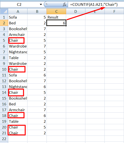
The function calculates the number of cells with indicated context, i.e., with the data that the user needs to count. For instance, you have a chart with diversified furniture bought over time. You may count what furniture (sofa, bed, wardrobe, chair, table, etc.) people buy. The COUNTIF will compute the cells in which the mentioned furniture is located. You write down the formula according to the condition you ought to detect. For example, let’s count the number of cells containing the word ‘chair‘:
=COUNTIF(A1:A21,"Chair")
Does COUNTIF function in Excel work for several criteria?
The COUNTIF doesn’t support frequentative conditions. Thus, you won’t find the number of chairs or nightstands purchased only in January or only on February 3. You have to use COUNTIFS for such cases.
However, you may write COUNTIF + COUNTIF. Such a COUNTIF Excel multiple criteria function makes the outcome more complete. Let’s determine the number of purchased chairs and sofas. Write the following:
=COUNTIF(A2:A21,"Chair")+COUNTIF(A2:A21,"Sofa").

Samples of advanced COUNTIFS function in Excel
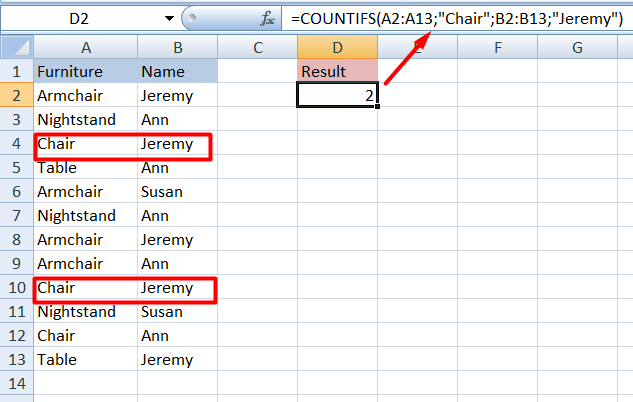
COUNTIF and COUNTIFS are various functions. They differ in the computation of cells with one criterion or more criteria. The first identifies cells under one condition, and the second takes into account several specific criteria. Let’s count the number of chairs bought by Jeremy. We need to use COUNTIFS for such appointments. Write it as follows:
=COUNTIFS(A2:A13,"Chair",B2:B13,"Jeremy")
Using COUNTIF in Excel when data is on other sources
People usually store data on certain apps, such as Harvest, Google Drive, Jira, Pipedrive, etc. When you need to calculate this data in Excel, you can import it from the app. The Coupler.io tool is designed exactly for this. It will help transfer all the necessary information to BigQuery, Google Sheets, or Excel from other sources. In addition, you can automate updates to make your work easier in the future.

Sign up to Coupler.io and complete two steps to set up your Excel integration: source and destination. If you want to schedule automatic data refresh, you’ll need to configure one more step – schedule. Here is what the integration may look like:

Practical skills based on a COUNTIF Excel example
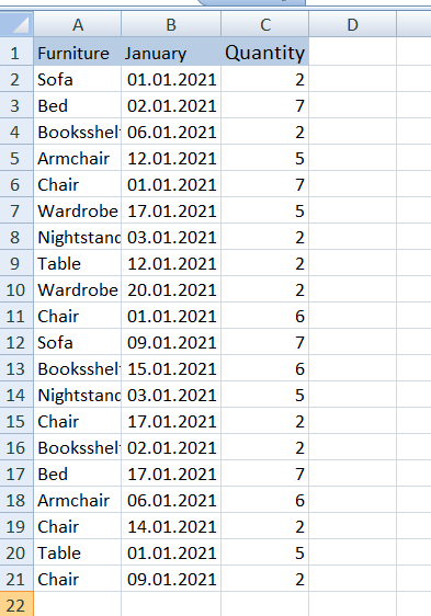
Examine a few samples of use in more detail. Take, for instance, the furniture in the store. Imagine the owner created an Excel table regarding sales. They write down the furniture in one column there. The other column contains the dates when the goods were sold. Finally, the third column contains the quantity of each product sold. So, let’s define some samples with several formulas, including dates, words and figures.
Excel COUNTIF: Cells are equal or not equal
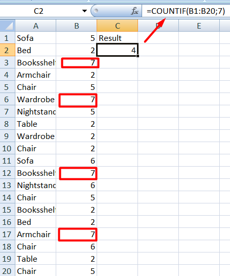
Imagine that people have bought every subject several times. Let’s take, for example, 7 times. In our formula, we specify the range where to look and the figure 7.
=COUNTIF(B1:B20,7)
Let’s still find the purchased furniture that isn’t equal to 5.
=COUNTIF(B1:B20,"<>5")

Excel COUNTIF: cells contain words
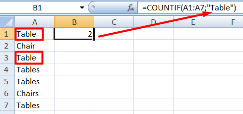
Let’s try to work with words using the same formula. Imagine that we need to know how many tables people bought. Let’s write the following formula.
=COUNTIF(A2:A21,"Table")

As a result, people bought 2 tables. You can replace the word with a cell reference
=COUNTIF(A2:A21,E2)

COUNTIF use in Excel – meaning of wildcards
We can use COUNTIF not only with words but also with special wildcards (* and ?) to generalize the condition.
?= One character.*= Sequence.
Also, you can write ~ to find symbols * or ?.
Let’s look at a simple formula
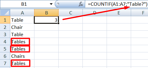
=COUNTIF(A1:A7,"Table")
The question mark symbol ? adds one additional character. In our dataset, there are the words ‘Table‘ and ‘Tables‘ with the last letter ‘s‘. So, Table? in the formula will look for the latter option:
=COUNTIF(A1:A7,"Table?")
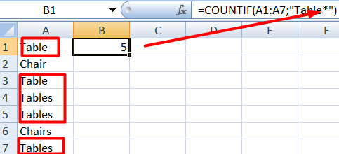
The asterisk symbol * adds a sequence of characters or even spaces. For instance, the following formula counts all words that start with Tab including ‘Table’ and ‘Tables’:
=COUNTIF(A1:A7,"Tab*")
Excel COUNTIF: сells are more than or less than
Let’s find out some values using operators: >, <, <>, =. We write it next to the criterion in quotation marks. Thanks to them, we can find cells with numbers that are more or less, equal, or not equal to some value. For example, let’s count the amount of furniture that people bought more than 3 times:
=COUNTIF(B1:B20,">3")

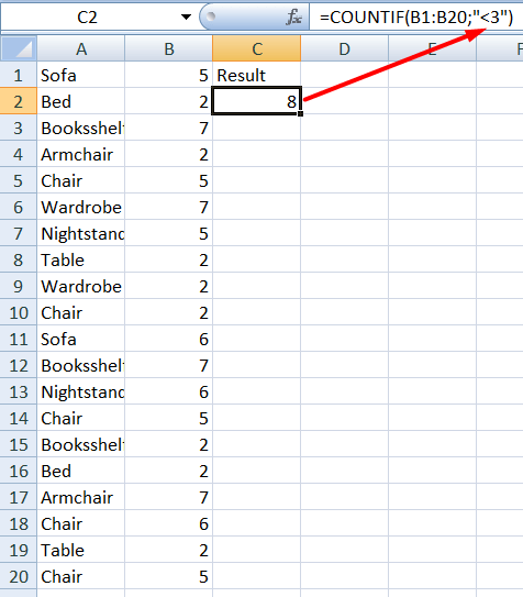
Change the logical operator to count the amount of furniture that people bought less than 3 times:
=COUNTIF(B1:B20,"<3")
Excel COUNTIF: count cells including date
Another feature is working with dates. So, let’s imagine that the biggest purchases fall on the date of January 1. We need to know the cells’ numerosity with this data.
=COUNTIF(B2:B21,"01/01/2021")

What common problems should you avoid?
Often, people face issues using the function. We seem to be doing everything right, but the Excel function COUNTIF shows the error. Look at a few situations why it occurs. For instance, you wrote the formula
=COUNTIF(A2:A13,Chair)
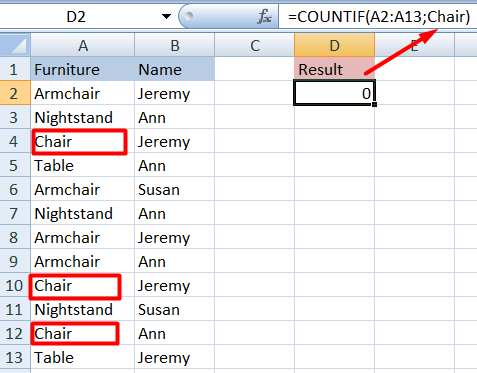
The function has shown zero results although this is not correct. So taking a closer look, the word ‘Chair‘ should be in quotation marks.
=COUNTIF(A2:A13,"Chair")
In another example of incorrect syntax, the formula returned #NAME?. In this case, there is a space between the range (A1:A7) and the criterion, which also has not quotation marks (Table).

The correct formula should look like this
=COUNTIF(A1:A7,"Table")
Best practices in using the COUNTIF function
It is easy to make mistakes both out of ignorance and inattention. However, by applying the following tips you can avoid the common mistakes.
- Write the wildcards (
?and*) to generalize the condition. - The condition can only have less than 255 characters. You will see an error exceeding this limit. To exceed the limit, you can use CONCATENATE or ampersand (&).
- The function returns the same value if the words are written in uppercase or lowercase letters. It doesn’t take into account case strings. You should rename the word if it has a different meaning.
- Pay attention to the spelling of words and letters. The function does not differentiate case strings and doesn’t work with misspellings.
Adherence to all principles and rules and writing correct syntax will facilitate calculations without problems. The main point is to write the formula and condition correctly.
-

Technical Content Writer on Coupler.io who loves working with data, writing about it, and even producing videos about it. I’ve worked at startups and product companies, writing content for technical audiences of all sorts. You’ll often see me cycling🚴🏼♂️, backpacking around the world🌎, and playing heavy board games.

Back to Blog
Focus on your business
goals while we take care of your data!
Try Coupler.io