
COUNTIF function
Use COUNTIF, one of the statistical functions, to count the number of cells that meet a criterion; for example, to count the number of times a particular city appears in a customer list.
In its simplest form, COUNTIF says:
-
=COUNTIF(Where do you want to look?, What do you want to look for?)
For example:
-
=COUNTIF(A2:A5,»London»)
-
=COUNTIF(A2:A5,A4)

COUNTIF(range, criteria)
|
Argument name |
Description |
|---|---|
|
range (required) |
The group of cells you want to count. Range can contain numbers, arrays, a named range, or references that contain numbers. Blank and text values are ignored. Learn how to select ranges in a worksheet. |
|
criteria (required) |
A number, expression, cell reference, or text string that determines which cells will be counted. For example, you can use a number like 32, a comparison like «>32», a cell like B4, or a word like «apples». COUNTIF uses only a single criteria. Use COUNTIFS if you want to use multiple criteria. |
Examples
To use these examples in Excel, copy the data in the table below, and paste it in cell A1 of a new worksheet.
|
Data |
Data |
|---|---|
|
apples |
32 |
|
oranges |
54 |
|
peaches |
75 |
|
apples |
86 |
|
Formula |
Description |
|
=COUNTIF(A2:A5,»apples») |
Counts the number of cells with apples in cells A2 through A5. The result is 2. |
|
=COUNTIF(A2:A5,A4) |
Counts the number of cells with peaches (the value in A4) in cells A2 through A5. The result is 1. |
|
=COUNTIF(A2:A5,A2)+COUNTIF(A2:A5,A3) |
Counts the number of apples (the value in A2), and oranges (the value in A3) in cells A2 through A5. The result is 3. This formula uses COUNTIF twice to specify multiple criteria, one criteria per expression. You could also use the COUNTIFS function. |
|
=COUNTIF(B2:B5,»>55″) |
Counts the number of cells with a value greater than 55 in cells B2 through B5. The result is 2. |
|
=COUNTIF(B2:B5,»<>»&B4) |
Counts the number of cells with a value not equal to 75 in cells B2 through B5. The ampersand (&) merges the comparison operator for not equal to (<>) and the value in B4 to read =COUNTIF(B2:B5,»<>75″). The result is 3. |
|
=COUNTIF(B2:B5,»>=32″)-COUNTIF(B2:B5,»<=85″) |
Counts the number of cells with a value greater than (>) or equal to (=) 32 and less than (<) or equal to (=) 85 in cells B2 through B5. The result is 1. |
|
=COUNTIF(A2:A5,»*») |
Counts the number of cells containing any text in cells A2 through A5. The asterisk (*) is used as the wildcard character to match any character. The result is 4. |
|
=COUNTIF(A2:A5,»?????es») |
Counts the number of cells that have exactly 7 characters, and end with the letters «es» in cells A2 through A5. The question mark (?) is used as the wildcard character to match individual characters. The result is 2. |
Common Problems
|
Problem |
What went wrong |
|---|---|
|
Wrong value returned for long strings. |
The COUNTIF function returns incorrect results when you use it to match strings longer than 255 characters. To match strings longer than 255 characters, use the CONCATENATE function or the concatenate operator &. For example, =COUNTIF(A2:A5,»long string»&»another long string»). |
|
No value returned when you expect a value. |
Be sure to enclose the criteria argument in quotes. |
|
A COUNTIF formula receives a #VALUE! error when referring to another worksheet. |
This error occurs when the formula that contains the function refers to cells or a range in a closed workbook and the cells are calculated. For this feature to work, the other workbook must be open. |
Best practices
|
Do this |
Why |
|---|---|
|
Be aware that COUNTIF ignores upper and lower case in text strings. |
|
|
Use wildcard characters. |
Wildcard characters —the question mark (?) and asterisk (*)—can be used in criteria. A question mark matches any single character. An asterisk matches any sequence of characters. If you want to find an actual question mark or asterisk, type a tilde (~) in front of the character. For example, =COUNTIF(A2:A5,»apple?») will count all instances of «apple» with a last letter that could vary. |
|
Make sure your data doesn’t contain erroneous characters. |
When counting text values, make sure the data doesn’t contain leading spaces, trailing spaces, inconsistent use of straight and curly quotation marks, or nonprinting characters. In these cases, COUNTIF might return an unexpected value. Try using the CLEAN function or the TRIM function. |
|
For convenience, use named ranges |
COUNTIF supports named ranges in a formula (such as =COUNTIF(fruit,»>=32″)-COUNTIF(fruit,»>85″). The named range can be in the current worksheet, another worksheet in the same workbook, or from a different workbook. To reference from another workbook, that second workbook also must be open. |
Note: The COUNTIF function will not count cells based on cell background or font color. However, Excel supports User-Defined Functions (UDFs) using the Microsoft Visual Basic for Applications (VBA) operations on cells based on background or font color. Here is an example of how you can Count the number of cells with specific cell color by using VBA.
Need more help?
You can always ask an expert in the Excel Tech Community or get support in the Answers community.

See also
COUNTIFS function
IF function
COUNTA function
Overview of formulas in Excel
IFS function
SUMIF function
Need more help?
Want more options?
Explore subscription benefits, browse training courses, learn how to secure your device, and more.
Communities help you ask and answer questions, give feedback, and hear from experts with rich knowledge.
In this example, the goal is to count cells in a range that contain text values. This could be hardcoded text like «apple» or «red», numbers entered as text, or formulas that return text values. Empty cells, and cells that contain numeric values or errors should not be included in the count. This problem can be solved with the COUNTIF function or the SUMPRODUCT function. Both approaches are explained below. For convenience, data is the named range B5:B15.
COUNTIF function
The simplest way to solve this problem is with the COUNTIF function and the asterisk (*) wildcard. The asterisk (*) matches zero or more characters of any kind. For example, to count cells in a range that begin with «a», you can use COUNTIF like this:
=COUNTIF(range,"a*") // begins with "a"
In this example however we don’t want to match any specific text value. We want to match all text values. To do this, we provide the asterisk (*) by itself for criteria. The formula in H5 is:
=COUNTIF(data,"*") // any text value
The result is 4, because there are four cells in data (B5:B15) that contain text values.
To reverse the operation of the formula and count all cells that do not contain text, add the not equal to (<>) logical operator like this:
=COUNTIF(data,"<>*") // non-text values
This is the formula used in cell H6. The result is 7, since there are seven cells in data (B5:B15) that do not contain text values.
COUNTIFS function
To apply more specific criteria, you can switch to the COUNTIFs function, which supports multiple conditions. For example, to count cells with text, but exclude cells that contain only a space character, you can use a formula like this:
=COUNTIFS(range,"*",range,"<> ")
This formula will count cells that contain any text value except a single space (» «).
SUMPRODUCT function
Another way to solve this problem is to use the SUMPRODUCT function with the ISTEXT function. SUMPRODUCT makes it easy to perform a logical test on a range, then count the results. The test is performed with the ISTEXT function. True to its name, the ISTEXT function only returns TRUE when given a text value:
=ISTEXT("apple")// returns TRUE
=ISTEXT(70) // returns FALSE
To count cells with text values in the example shown, you can use a formula like this:
=SUMPRODUCT(--ISTEXT(data))
Working from the inside out, the logical test is based on the ISTEXT function:
ISTEXT(data)
Because data (B5:B15) contains 11 values, ISTEXT returns 11 results in an array like this:
{TRUE;TRUE;TRUE;FALSE;FALSE;TRUE;FALSE;FALSE;FALSE;FALSE;FALSE}
In this array, the TRUE values correspond to cells that contain text values, and the FALSE values represent cells that do not contain text. To convert the TRUE and FALSE values to 1s and 0s, we use a double negative (—):
--{TRUE;TRUE;TRUE;FALSE;FALSE;TRUE;FALSE;FALSE;FALSE;FALSE;FALSE}
The resulting array inside the SUMPRODUCT function looks like this:
=SUMPRODUCT({1;1;1;0;0;1;0;0;0;0;0}) // returns 4
With a single array to process, SUMPRODUCT sums the array and returns 4 as the result.
To reverse the formula and count all cells that do not contain text, you can nest the ISTEXT function inside the NOT function like this:
=SUMPRODUCT(--NOT(ISTEXT(data)))
The NOT function reverses the results from ISTEXT. The double negative (—) converts the array to numbers, and the array inside SUMPRODUCT looks like this:
=SUMPRODUCT({0;0;0;1;1;0;1;1;1;1;1}) // returns 7
The result is 7, since there are seven cells in data (B5:B15) that do not contain text values.
Note: the SUMPRODUCT formulas above may seem complex, but using Boolean operations in array formulas is powerful and flexible. It is also an important skill in modern functions like FILTER and XLOOKUP, which often use this technique to select the right data. The syntax used by COUNTIF on the other hand is unique to a group of eight functions and is therefore not as useful or portable.
Excel spreadsheet is known to be one of the best data storing and analyzing tools. Cells together make spreadsheets that consist of text and numbers. For more understanding, you have to differentiate cells filled with text.
So, practically how would you count cells with text in Excel? You can use a few different formulas to count cells containing any text, empty cells, and cells with specific characters or just filtered cells. All these formulas can be used in Excel 2019, 2016, 2013, and 2010.
At first, Excel spreadsheets were limited to dealing with numbers, however now we can use these sheets to store as well as modify text. Do you really want to know how many cells are filled with text in your data sheet?
For this purpose, you can use multiple functions in Excel. Depending on the situation, you can use any function.
Here you will find the tricks to count text in Excel. Let’s have a look at how you can count if a cell contains text in different conditions.
Before moving forward to learn how Excel counts cells with text, why not have a quick overview of what a Count If the function is.
COUNTIF Function
To be honest, counting cells containing text in a spreadsheet is not an easy task. That’s why the Count if the function is there to help you in this case. Using asterisk wildcards, you can count the number of cells having specific text with COUNTIF function.
The basic purpose of asterisk wildcards is to correspond to any characters or numbers. Putting them before and after any text, you can simply count the number of cells in which the text is found.
Here is the general formula for the COUNTIF function:
=COUNTIF (Range, “*Text*”)
Example:
=COUNTIF (A2:A11, “*Class*”)
The last name “Class” when put in the asterisk, the COUNTIF formula simply calculates all string values within the range containing the name “Class.”

How to Count Number of Cells with Text in Excel
You can count if cell contains any text string or character by using two basic formulas.
Using COUNTIF Formula to Count All Cells with Text
The COUNTIF formula with an asterisk in the criteria argument is the main solution. For instance:
COUNTIF (range, “*”) (as mentioned above)
For more understanding of this formula, let’s have a look at which values are included and which are not:
Counted Values
- Special characters
- Cells with all kinds of text
- Numbers formatted as text
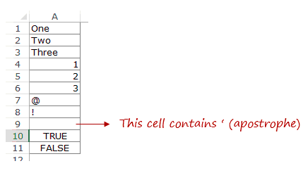
- Visually blank cells that have an empty string (“”), apostrophe (‘), space, or non-printing characters
Non-Counted Values
- Numbers
- Errors
- Dates
- Blank cells
- Logical values of TRUE or FALSE
For instance, in the range A2:A10, you can count if the cell contains text, apart from dates, numbers, logical values, blank cells, and errors.
Try using one of the following formulas:
COUNTIF(A2:A10, “*”)
SUMPRODUCT(–ISTEXT(A2:A10))
SUMPRODUCT( ISTEXT(A2:A10)*1)

Count If Cell Contains Text without Spaces and Empty Strings
Using the above-mentioned formulas can help you count all cells containing any text or character in them. However, in some situations, it might be tiring and confusing as certain cells may look blank, but in reality, they are not.
Keep in mind that empty strings, spaces, apostrophes, line breaks, etc are not easily countable with the human eye. However, they are not difficult to count using formulas.
Using the COUNTIFS function will let you exclude “false positive” blank cells from the count. For instance, in the range A2:A7, you can count cells with text that overlooks the space character:
COUNTIFS(A2:A7l”*”A2:A7,”<>”)

If your target range has any formula-driven data, it might be possible that some of the formulas can ultimately be an empty string (“”). You can even ignore these empty strings by replacing “*” with “*?*” in the criteria 1 argument:
=COUNTIFS(A2:A9,”*?*”, A2:A9, “<>”)
Here the question mark shows that you need to have at least one text character. You know that an empty string does not have characters in it, and it does not meet that’s why it is not included. Also, remember that blank cells starting with an apostrophe (‘) are not included as well.
Below in the image, you can see a space in A7 cell, an apostrophe in A8, and an empty string (=””) in A9.

How to Count IF Cells Contain Specific Text
As you already know that COUNTIF function is best for counting all cells containing text, you can even COUNTIF cell contains specific text. Suppose, we need to count the number of times the word used “Excel” in a specific cell range:
- Open the spreadsheet in Excel you want to check.
- Click on a blank cell to enter the formula.

- In the blank cell, you need to type “=COUNTIF (range, criteria)”.
Using this formula will count all the number of cells having specific text within a cell range.

- You have to enter the cell range you need to count for the “range”. Now, add the first and last cells separated with a colon. Enter “A2: A20” to count cells.

- Now type “Excel” for the “Criteria.” It will help you count the number of cells using “Excel” in a certain range. Your formula will look like “=COUNTIF (A2:A20, “Excel”).

How To Count Cells with Color Text in Excel
Do you know Excel does not provide a formula to count cells with colored text?
However, still you cannot do this manually as counting all colored cells one by one is not an easy thing. By filtering the results, you can execute this process. Follow the steps given below:
- Go to the spreadsheet you want to analyze.

- Right-click a cell with the text of the color you want to count.

- Select “Filter,” and then “Filter by Selected Cell’s Font Color” to filter the cells with the selected text color.

- Get ready for counting the data range. Here is the formula if your text is from cell B2 to B20: “=SUBTOTAL (B2:B20)”

After pressing the “Enter” key, your filter will be applied and Excel will start showing the cells having that specific color and the remaining value–s will be hidden.
In the hidden rows, the “SUBTOTAL” function will not add the values. That’s why it will only count the selected color text.
Summing Up Count If Cell Contains Text
For storing and analyzing the data, Excel is a huge platform that provides multiple functions for several problems. Both text and numbers are dealt in Excel. Around four hundred functions can use the COUNTIF function. It helps in finding the sum of cells containing specific data.
17 авг. 2022 г.
читать 2 мин
Вы можете использовать следующие методы для подсчета ячеек в Excel, содержащих определенный текст:
Метод 1: подсчет ячеек, содержащих один конкретный текст
=COUNTIF( A2:A13 , "*text*")
Эта формула будет подсчитывать количество ячеек в диапазоне A2:A13 , которые содержат «текст» в ячейке.
Метод 2: подсчет ячеек, содержащих один из нескольких текстов
=SUM(COUNTIF( A2:A13 ,{"*text1","*text2*","*text3*"}))
Эта формула будет подсчитывать количество ячеек в диапазоне A2:A13 , которые содержат «текст1», «текст2» или «текст3» в ячейке.
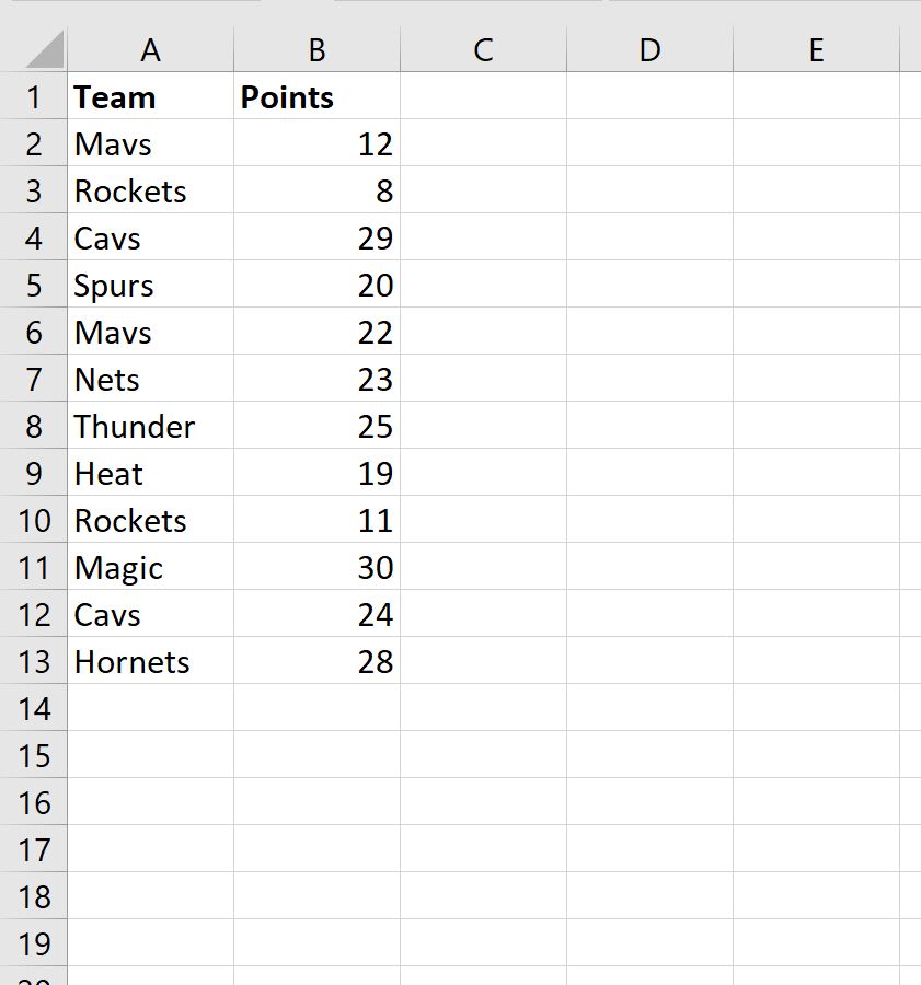
В следующих примерах показано, как использовать каждый метод на практике со следующим набором данных в Excel:
Пример 1. Подсчет ячеек, содержащих один конкретный текст
Мы можем использовать следующую формулу для подсчета значений в столбце Team , которые содержат «avs» в названии:
=COUNTIF( A2:A13 , "*avs*")
На следующем снимке экрана показано, как использовать эту формулу на практике:
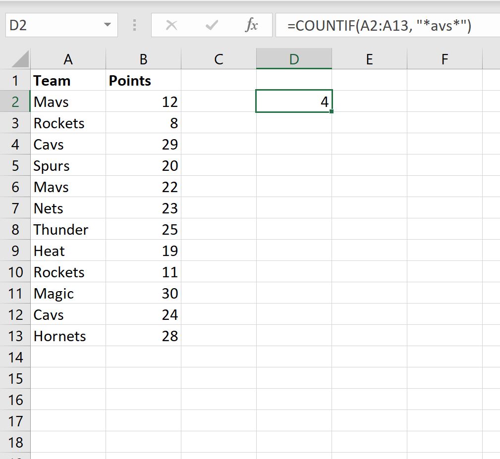
Мы видим, что всего 4 ячейки в столбце « Команда » содержат «avs» в названии.
Пример 2. Подсчет ячеек, содержащих один из нескольких текстов
Мы можем использовать следующую формулу для подсчета количества ячеек в столбце Team , которые содержат «avs», «urs» или «pockets» в имени:
=SUM(COUNTIF( A2:A13 ,{"*avs","*urs*","*ockets*"}))
На следующем снимке экрана показано, как использовать эту формулу на практике:
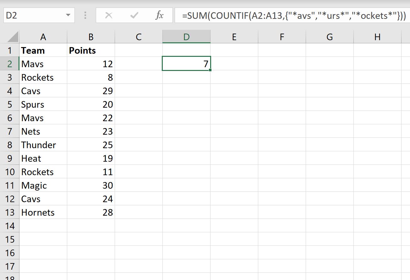
Мы видим, что в общей сложности 7 ячеек в столбце « Команда » содержат «avs», «urs» или «pockets» в названии.
Дополнительные ресурсы
В следующих руководствах объясняется, как выполнять другие распространенные задачи в Excel:
Excel: как удалить строки с определенным текстом
Excel: как проверить, содержит ли ячейка частичный текст
Excel: как проверить, содержит ли ячейка текст из списка
Excel has many functions where a user needs to specify a single or multiple criteria to get the result. For example, if you want to count cells based on multiple criteria, you can use the COUNTIF or COUNTIFS functions in Excel.
This tutorial covers various ways of using a single or multiple criteria in COUNTIF and COUNTIFS function in Excel.
While I will primarily be focussing on COUNTIF and COUNTIFS functions in this tutorial, all these examples can also be used in other Excel functions that take multiple criteria as inputs (such as SUMIF, SUMIFS, AVERAGEIF, and AVERAGEIFS).
An Introduction to Excel COUNTIF and COUNTIFS Functions
Let’s first get a grip on using COUNTIF and COUNTIFS functions in Excel.
Excel COUNTIF Function (takes Single Criteria)
Excel COUNTIF function is best suited for situations when you want to count cells based on a single criterion. If you want to count based on multiple criteria, use COUNTIFS function.
Syntax
=COUNTIF(range, criteria)
Input Arguments
- range – the range of cells which you want to count.
- criteria – the criteria that must be evaluated against the range of cells for a cell to be counted.
Excel COUNTIFS Function (takes Multiple Criteria)
Excel COUNTIFS function is best suited for situations when you want to count cells based on multiple criteria.
Syntax
=COUNTIFS(criteria_range1, criteria1, [criteria_range2, criteria2]…)
Input Arguments
- criteria_range1 – The range of cells for which you want to evaluate against criteria1.
- criteria1 – the criteria which you want to evaluate for criteria_range1 to determine which cells to count.
- [criteria_range2] – The range of cells for which you want to evaluate against criteria2.
- [criteria2] – the criteria which you want to evaluate for criteria_range2 to determine which cells to count.
Now let’s have a look at some examples of using multiple criteria in COUNTIF functions in Excel.
Using NUMBER Criteria in Excel COUNTIF Functions
#1 Count Cells when Criteria is EQUAL to a Value
To get the count of cells where the criteria argument is equal to a specified value, you can either directly enter the criteria or use the cell reference that contains the criteria.
Below is an example where we count the cells that contain the number 9 (which means that the criteria argument is equal to 9). Here is the formula:
=COUNTIF($B$2:$B$11,D3)

In the above example (in the pic), the criteria is in cell D3. You can also enter the criteria directly into the formula. For example, you can also use:
=COUNTIF($B$2:$B$11,9)
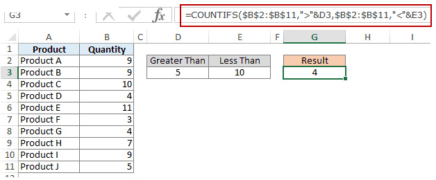
#2 Count Cells when Criteria is GREATER THAN a Value
To get the count of cells with a value greater than a specified value, we use the greater than operator (“>”). We could either use it directly in the formula or use a cell reference that has the criteria.
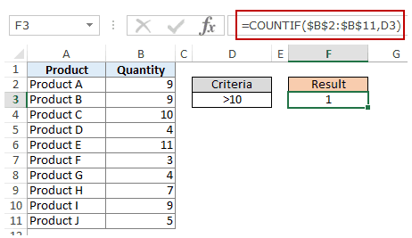
Whenever we use an operator in criteria in Excel, we need to put it within double quotes. For example, if the criteria is greater than 10, then we need to enter “>10” as the criteria (see pic below):
Here is the formula:
=COUNTIF($B$2:$B$11,”>10″)

You can also have the criteria in a cell and use the cell reference as the criteria. In this case, you need NOT put the criteria in double quotes:
=COUNTIF($B$2:$B$11,D3)
There could also be a case when you want the criteria to be in a cell, but don’t want it with the operator. For example, you may want the cell D3 to have the number 10 and not >10.
In that case, you need to create a criteria argument which is a combination of operator and cell reference (see pic below):
=COUNTIF($B$2:$B$11,”>”&D3)
 NOTE: When you combine an operator and a cell reference, the operator is always in double quotes. The operator and cell reference are joined by an ampersand (&).
#3 Count Cells when Criteria is LESS THAN a Value
To get the count of cells with a value less than a specified value, we use the less than operator (“<“). We could either use it directly in the formula or use a cell reference that has the criteria.
Whenever we use an operator in criteria in Excel, we need to put it within double quotes. For example, if the criterion is that the number should be less than 5, then we need to enter “<5” as the criteria (see pic below):
=COUNTIF($B$2:$B$11,”<5″)

You can also have the criteria in a cell and use the cell reference as the criteria. In this case, you need NOT put the criteria in double quotes (see pic below):
=COUNTIF($B$2:$B$11,D3)

Also, there could be a case when you want the criteria to be in a cell, but don’t want it with the operator. For example, you may want the cell D3 to have the number 5 and not <5.
In that case, you need to create a criteria argument which is a combination of operator and cell reference:
=COUNTIF($B$2:$B$11,”<“&D3)

NOTE: When you combine an operator and a cell reference, the operator is always in double quotes. The operator and cell reference are joined by an ampersand (&).
#4 Count Cells with Multiple Criteria – Between Two Values
To get a count of values between two values, we need to use multiple criteria in the COUNTIF function.
Here are two methods of doing this:
METHOD 1: Using COUNTIFS function
COUNTIFS function can handle multiple criteria as arguments and counts the cells only when all the criteria are TRUE. To count cells with values between two specified values (say 5 and 10), we can use the following COUNTIFS function:
=COUNTIFS($B$2:$B$11,”>5″,$B$2:$B$11,”<10″)

NOTE: The above formula does not count cells that contain 5 or 10. If you want to include these cells, use greater than equal to (>=) and less than equal to (<=) operators. Here is the formula:
=COUNTIFS($B$2:$B$11,”>=5″,$B$2:$B$11,”<=10″)
You can also have these criteria in cells and use the cell reference as the criteria. In this case, you need NOT put the criteria in double quotes (see pic below):

You can also use a combination of cells references and operators (where the operator is entered directly in the formula). When you combine an operator and a cell reference, the operator is always in double quotes. The operator and cell reference are joined by an ampersand (&).
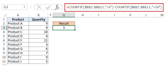
METHOD 2: Using two COUNTIF functions
If you have multiple criteria, you can either use COUNTIFS or create a combination of COUNTIF functions. The formula below would also do the same thing:
=COUNTIF($B$2:$B$11,”>5″)-COUNTIF($B$2:$B$11,”>10″)
In the above formula, we first find the number of cells that have a value greater than 5 and we subtract the count of cells with a value greater than 10. This would give us the result as 5 (which is the number of cells that have values more than 5 and less than equal to 10).
If you want the formula to include both 5 and 10, use the following formula instead:
=COUNTIF($B$2:$B$11,”>=5″)-COUNTIF($B$2:$B$11,”>10″)
If you want the formula to exclude both ‘5’ and ’10’ from the counting, use the following formula:
=COUNTIF($B$2:$B$11,”>=5″)-COUNTIF($B$2:$B$11,”>10″)-COUNTIF($B$2:$B$11,10)
You can have these criteria in cells and use the cells references, or you can use a combination of operators and cells references.
Using TEXT Criteria in Excel Functions
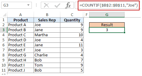
#1 Count Cells when Criteria is EQUAL to a Specified text
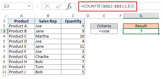
To count cells that contain an exact match of the specified text, we can simply use that text as the criteria. For example, in the dataset (shown below in the pic), if I want to count all the cells with the name Joe in it, I can use the below formula:
=COUNTIF($B$2:$B$11,”Joe”)
Since this is a text string, I need to put the text criteria in double quotes.
You can also have the criteria in a cell and then use that cell reference (as shown below):
=COUNTIF($B$2:$B$11,E3)

NOTE: You can get wrong results if there are leading/trailing spaces in the criteria or criteria range. Make sure you clean the data before using these formulas.
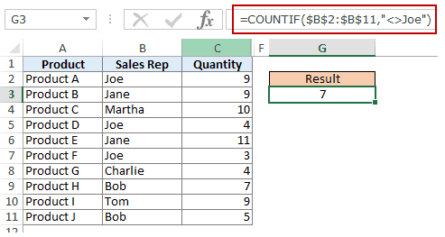
#2 Count Cells when Criteria is NOT EQUAL to a Specified text
Similar to what we saw in the above example, you can also count cells that do not contain a specified text. To do this, we need to use the not equal to operator (<>).
Suppose you want to count all the cells that do not contain the name JOE, here is the formula that will do it:
=COUNTIF($B$2:$B$11,”<>Joe”)
You can also have the criteria in a cell and use the cell reference as the criteria. In this case, you need NOT put the criteria in double quotes (see pic below):
=COUNTIF($B$2:$B$11,E3)
There could also be a case when you want the criteria to be in a cell but don’t want it with the operator. For example, you may want the cell D3 to have the name Joe and not <>Joe.
In that case, you need to create a criteria argument which is a combination of operator and cell reference (see pic below):
=COUNTIF($B$2:$B$11,”<>”&E3)
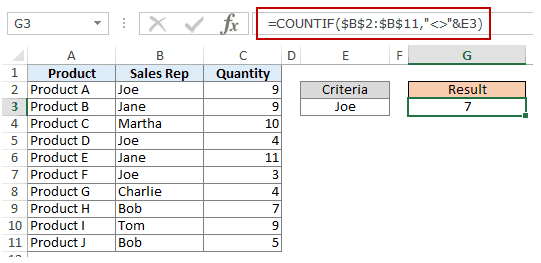
When you combine an operator and a cell reference, the operator is always in double quotes. The operator and cell reference are joined by an ampersand (&).
Using DATE Criteria in Excel COUNTIF and COUNTIFS Functions
Excel store date and time as numbers. So we can use it the same way we use numbers.
#1 Count Cells when Criteria is EQUAL to a Specified Date
To get the count of cells that contain the specified date, we would use the equal to operator (=) along with the date.
To use the date, I recommend using the DATE function, as it gets rid of any possibility of error in the date value. So, for example, if I want to use the date September 1, 2015, I can use the DATE function as shown below:
=DATE(2015,9,1)
This formula would return the same date despite regional differences. For example, 01-09-2015 would be September 1, 2015 according to the US date syntax and January 09, 2015 according to the UK date syntax. However, this formula would always return September 1, 2105.
Here is the formula to count the number of cells that contain the date 02-09-2015:
=COUNTIF($A$2:$A$11,DATE(2015,9,2))

#2 Count Cells when Criteria is BEFORE or AFTER to a Specified Date
To count cells that contain date before or after a specified date, we can use the less than/greater than operators.
For example, if I want to count all the cells that contain a date that is after September 02, 2015, I can use the formula:
=COUNTIF($A$2:$A$11,”>”&DATE(2015,9,2))

Similarly, you can also count the number of cells before a specified date. If you want to include a date in the counting, use and ‘equal to’ operator along with ‘greater than/less than’ operator.
You can also use a cell reference that contains a date. In this case, you need to combine the operator (within double quotes) with the date using an ampersand (&).
See example below:
=COUNTIF($A$2:$A$11,”>”&F3)

#3 Count Cells with Multiple Criteria – Between Two Dates
To get a count of values between two values, we need to use multiple criteria in the COUNTIF function.
We can do this using two methods – One single COUNTIFS function or two COUNTIF functions.
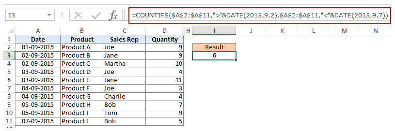
METHOD 1: Using COUNTIFS function
COUNTIFS function can take multiple criteria as the arguments and counts the cells only when all the criteria are TRUE. To count cells with values between two specified dates (say September 2 and September 7), we can use the following COUNTIFS function:
=COUNTIFS($A$2:$A$11,”>”&DATE(2015,9,2),$A$2:$A$11,”<“&DATE(2015,9,7))
The above formula does not count cells that contain the specified dates. If you want to include these dates as well, use greater than equal to (>=) and less than equal to (<=) operators. Here is the formula:
=COUNTIFS($A$2:$A$11,”>=”&DATE(2015,9,2),$A$2:$A$11,”<=”&DATE(2015,9,7))
You can also have the dates in a cell and use the cell reference as the criteria. In this case, you can not have the operator with the date in the cells. You need to manually add operators in the formula (in double quotes) and add cell reference using an ampersand (&). See the pic below:
=COUNTIFS($A$2:$A$11,”>”&F3,$A$2:$A$11,”<“&G3)

METHOD 2: Using COUNTIF functions
If you have multiple criteria, you can either use one COUNTIFS function or create a combination of two COUNTIF functions. The formula below would also do the trick:
=COUNTIF($A$2:$A$11,”>”&DATE(2015,9,2))-COUNTIF($A$2:$A$11,”>”&DATE(2015,9,7))
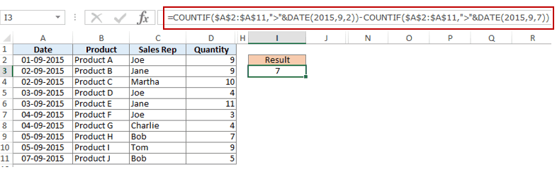
In the above formula, we first find the number of cells that have a date after September 2 and we subtract the count of cells with dates after September 7. This would give us the result as 7 (which is the number of cells that have dates after September 2 and on or before September 7).
If you don’t want the formula to count both September 2 and September 7, use the following formula instead:
=COUNTIF($A$2:$A$11,”>=”&DATE(2015,9,2))-COUNTIF($A$2:$A$11,”>”&DATE(2015,9,7))

If you want to exclude both the dates from counting, use the following formula:
=COUNTIF($A$2:$A$11,”>”&DATE(2015,9,2))-COUNTIF($A$2:$A$11,”>”&DATE(2015,9,7)-COUNTIF($A$2:$A$11,DATE(2015,9,7)))
Also, you can have the criteria dates in cells and use the cells references (along with operators in double quotes joined using ampersand).
Using WILDCARD CHARACTERS in Criteria in COUNTIF & COUNTIFS Functions
There are three wildcard characters in Excel:
- * (asterisk) – It represents any number of characters. For example, ex* could mean excel, excels, example, expert, etc.
- ? (question mark) – It represents one single character. For example, Tr?mp could mean Trump or Tramp.
- ~ (tilde) – It is used to identify a wildcard character (~, *, ?) in the text.
You can use COUNTIF function with wildcard characters to count cells when other inbuilt count function fails. For example, suppose you have a data set as shown below:
Now let’s take various examples:
#1 Count Cells that contain Text
To count cells with text in it, we can use the wildcard character * (asterisk). Since asterisk represents any number of characters, it would count all cells that have any text in it. Here is the formula:
=COUNTIFS($C$2:$C$11,”*”)
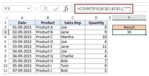
Note: The formula above ignores cells that contain numbers, blank cells, and logical values, but would count the cells contain an apostrophe (and hence appear blank) or cells that contain empty string (=””) which may have been returned as a part of a formula.
Here is a detailed tutorial on handling cases where there is an empty string or apostrophe.
Here is a detailed tutorial on handling cases where there are empty strings or apostrophes.
Below is a video that explains different scenarios of counting cells with text in it.
#2 Count Non-blank Cells
If you are thinking of using COUNTA function, think again.
Try it and it might fail you. COUNTA will also count a cell that contains an empty string (often returned by formulas as =”” or when people enter only an apostrophe in a cell). Cells that contain empty strings look blank but are not, and thus counted by the COUNTA function.
COUNTA will also count a cell that contains an empty string (often returned by formulas as =”” or when people enter only an apostrophe in a cell). Cells that contain empty strings look blank but are not, and thus counted by the COUNTA function.
So if you use the formula =COUNTA(A1:A11), it returns 11, while it should return 10.
Here is the fix:
=COUNTIF($A$1:$A$11,”?*”)+COUNT($A$1:$A$11)+SUMPRODUCT(–ISLOGICAL($A$1:$A$11))
Let’s understand this formula by breaking it down:
#3 Count Cells that contain specific text
Let’s say we want to count all the cells where the sales rep name begins with J. This can easily be achieved by using a wildcard character in COUNTIF function. Here is the formula:
=COUNTIFS($C$2:$C$11,”J*”)

The criteria J* specifies that the text in a cell should begin with J and can contain any number of characters.
If you want to count cells that contain the alphabet anywhere in the text, flank it with an asterisk on both sides. For example, if you want to count cells that contain the alphabet “a” in it, use *a* as the criteria.
This article is unusually long compared to my other articles. Hope you have enjoyed it. Let me know your thoughts by leaving a comment.
You May Also Find the following Excel tutorials useful:
- Count the number of words in Excel.
- Count Cells Based on Background Color in Excel.
- How to Sum a Column in Excel (5 Really Easy Ways)
You can use the following methods to count cells in Excel that contain specific text:
Method 1: Count Cells that Contain One Specific Text
=COUNTIF(A2:A13, "*text*")
This formula will count the number of cells in the range A2:A13 that contain “text” in the cell.
Method 2: Count Cells that Contain One of Several Text
=SUM(COUNTIF(A2:A13,{"*text1","*text2*","*text3*"}))
This formula will count the number of cells in the range A2:A13 that contain “text1”, “text2”, or “text3” in the cell.
The following examples show how to use each method in practice with the following dataset in Excel:

Example 1: Count Cells that Contain One Specific Text
We can use the following formula to count the values in the Team column that contain “avs” in the name:
=COUNTIF(A2:A13, "*avs*")
The following screenshot shows how to use this formula in practice:

We can see that a total of 4 cells in the Team column contain “avs” in the name.
Example 2: Count Cells that Contain One of Several Text
We can use the following formula to count the number of cells in the Team column that contain “avs”, “urs”, or “ockets” in the name:
=SUM(COUNTIF(A2:A13,{"*avs","*urs*","*ockets*"}))
The following screenshot shows how to use this formula in practice:

We can see that a total of 7 cells in the Team column contain “avs”, “urs”, or “ockets” in the name.
Additional Resources
The following tutorials explain how to perform other common tasks in Excel:
Excel: How to Delete Rows with Specific Text
Excel: How to Check if Cell Contains Partial Text
Excel: How to Check if Cell Contains Text from List

=COUNTIF(A2:A7,«*apple*») // criteria within formula
=COUNTIF(A:A,«*»&C6&«*») // criteria as a cell reference
A2:A7 & A:A = ranges
Check below for a detailed explanation with pictures and how to use formulas in Excel and Google Sheets.
Count if cells contain a specific text in Excel
Count if cells contain a specific text in Excel
How to count if cells contain a specific text in Excel?

COUNT IF CELLS CONTAIN A SPECIFIC TEXT — EXCEL FORMULA AND EXAMPLE
COUNT IF CELLS CONTAIN A SPECIFIC TEXT — EXCEL FORMULA AND EXAMPLE
-
=COUNTIF(A2:A7,«*apple*») // criteria within formula
-
=COUNTIF(A:A,«*»&C6&«*») // criteria as a cell reference
-
A2:A6 = data range
-
«*apple*» = criteria
-
Wildcard: The * character allows for any number (including zero) of other characters to take its place.
💡 In this example, it’s used to find all cells that include the text «apple». This search is not case-sensitive, so «apple» is considered the same as «Apple» or «APPLE».
Count if cells contain a specific text in Google Sheets
Count if cells contain a specific text in Google Sheets
How to count if cells contain specific text in Google Sheets?

COUNT IF CELLS CONTAIN A SPECIFIC TEXT — GOOGLE SHEETS FORMULA AND EXAMPLE
COUNT IF CELLS CONTAIN A SPECIFIC TEXT — GOOGLE SHEETS FORMULA AND EXAMPLE
-
=COUNTIF(A2:A7,«*apple*») // criteria within formula
-
=COUNTIF(A:A,«*»&C6&«*») // criteria as a cell reference
-
A2:A6 = data range
-
«*apple*» = criteria
-
Wildcard: The * character allows for any number (including zero) of other characters to take its place.
💡 In this example, it’s used to find all cells that include the text «apple». This search is not case-sensitive, so «apple» is considered the same as «Apple» or «APPLE».
Other useful «COUNT FUNCTIONS: TEXT BASED CRITERIA» formulas in Excel and Google Sheets
- Count cells in the column that have the same first five characters
- Count cells over 10 characters
- Count cells that are not blank
- Count cells that begin with a specific text
- Count cells that contain a specific text and ignore blank
- Count cells that contain errors
- Count if cells start with a specific text
- Count if cells end with a specific text
- Count the number of words in a cell
- Count the number of cells that have more than 5 characters words
- Count the number of occurrences of a text string in a range
- Count words in a range of cells and columns
- COUNTIF based on multiple criteria
Others Formulas
- Sum by month
- SUMIF cells if contains part of a text string
- Sum total sales based on quantity & price
- Combine date and time
- Convert 1-12 to month name
- Dynamic current date and time
- Count blank cell
- Count cell between two values
- Combine two or more cell
- Extract left before first space
- Extract the nth words in a text string
- Flip the first and last name
- SUMIF formulas and example
- SUMIFS formulas and example
- COUNTIF formulas and example
- IF formulas and example
- TEXT formulas and example
- CONVERT formulas and example
- Change the negative number to zero
- Change negative to positive numbers
- Calculate percentage changes for containing zero or negative values
Date and time functions
- Convert date to text
- Convert time to text
- Convert weekday string to number
- Combine two or more cells with a line break
- Combine two or more cells and transpose
Number based criteria
- Count cell between two values
- Count number of days between dates
Extract functions
- Get text between colons
- Transpose column to row
- Transpose row to column
Coming | Subscribe here for the custom Excel/Sheets formulas E-book (PDF) >
Google Sites
Report abuse
Table of Contents
- INTRODUCTION
- HOW TEXT IS HANDLED IN EXCEL?
- BASICS OF EXCEL COUNTIF TEXT CRITERIA
- EXAMPLE 1: COUNTING THE NUMBER OF REPETITIONS OF A PARTICULAR TEXT USING EXCEL COUNTIF TEXT CRITERIA
- EXAMPLE 2: COUNTING THE RESEMBLING WORDS USING EXCEL COUNTIF TEXT CRITERIA
- HOW TO COUNT THE WORDS STARTING WITH THE SAME LETTERS USING EXCEL COUNTIF TEXT CRITERIA?
- HOW TO COUNT THE WORDS ENDING WITH THE SAME LETTERS USING EXCEL COUNTIF TEXT CRITERIA?
- HOW TO COUNT THE WORDS CONTAINING THE SAME PATTERNS IN EXCEL?
- HOW TO USE COUNTIF FUNCTION IN EXCEL TO COUNT WORDS USING WILDCARD CHARACTERS?
INTRODUCTION
In this article, we’ll learn about the Excel countif text criteria i.e. using the COUNTIF FUNCTION with text values in Excel.
Countif is a very versatile function which can be used carry out a number of difficult tasks within a fraction of seconds. But we must know the way to make use of this function in the useful ways.
You can learn COUNTIF FUNCTION HERE which is recommended to get a better grasp of the trick being discussed here.
We make use of excel countif text criteria to compare the text values and make a count. The conditions can be many such as any text equal to or containing some portion or substring of other text etc.
LEARN MANY TRICKS WITH GYANKOSH.NET@ MANIPULATING TEXT IN EXCEL – PART I
HERE, WE WOULD LEARN ABOUT THE USAGE OF COUNTIF FUNCTION WITH TEXT TO GET SOME EXCITING RESULTS.
HOW TEXT IS HANDLED IN EXCEL?
TEXT is simply the group of characters and strings of characters that convey the information about the different data and numbers in Excel. Every character is connected with a code [ANSI].
Text comprises of the individual entity character which is the smallest bit which would be found in Excel.We can perform the operations on the strings[Text] or the characters. Characters are not limited to A to Z or a to z but many symbols are also included in this which we would see in the later part of the article.
TEXT IS AN INACTIVE NUMBER TYPE[FORMAT] IN EXCEL. ANYTHING STORED AS TEXT [NUMBER OR DATE] WON’T RESPOND TO ANY STANDARD FORMULAS OR FUNCTIONS BUT SPECIALLY DESIGNED TEXT FUNCTIONS. [EXCEPTIONS DO OCCUR IN CASE OF NUMBERS]
If we need to make anything inactive, such as Date to be nonresponding to the calculation, we put it as a text. Similarly if we want to avoid any calculations for a number it needs to be put as a text.
BASICS OF EXCEL COUNTIF TEXT CRITERIA
COUNTIF FUNCTION counts the values which fulfill the given conditions.
For example, count the numbers from a given data which is smaller than a particular value, or larger than a fixed value or equal to any value etc.
In this section we would focus upon the cases where the conditions will be put on the text rather than numerical values.
Let us learn the excel countif text criteria with the help of few examples.
EXAMPLE 1: COUNTING THE NUMBER OF REPETITIONS OF A PARTICULAR TEXT USING EXCEL COUNTIF TEXT CRITERIA
Let us take a data and find out the repetition of a particular word within the given data.
The data is as given below. These are the names of the places. Some of them are repeated.
WASHINGTON
PARIS
DELHI
DELHI
WASHINGTON
MOSCOW
ROME
ROME
MOSCOW
STEPS TO FIND THE NUMBER OF REPETITIONS OF A PARTICULAR TEXT (“WASHINGTON”)
- Select the cell where you want the result.
- Put the function as =COUNTIF(RANGE,”TEXT”)
For our example, the formula will be
=COUNTIF(F3:F11,G3) [Check picture below for cell references ]
for the first example where we are trying to find out the number of times WASHINGTON is repeated.
The first argument is the array reference which covers all the data in which we have to find out the repetitions ].
The second argument is the condition that we want to find. In our case, we have put the reference of the text we want to find.
We can also put “WASHINGTON” directly.
THE COMPARISON OF TEXT VALUE IN THE COUNTIF FUNCTION IGNORES THE CASE AND TREATS UPPER AND LOWER CASE AS EQUALS.
We extended the example to find out the number of repetitions of all the given places names.

EXAMPLE 2: COUNTING THE RESEMBLING WORDS USING EXCEL COUNTIF TEXT CRITERIA
Suppose we have the following group of words and we need to find out the resembling words.
A word can resemble in many ways.
Many words can have same prefixes, same suffixes, any pattern
Let us try different combinations.
GENERAL FORMULA TO COUNT THE WORDS HAVING SAME PREFIX:
=COUNTIF(RANGE,”PREFIX*”) PREFIX is the letters of the prefix.
GENERAL FORMULA TO COUNT THE WORDS HAVING SAME SUFFIX:
=COUNTIF(RANGE,”* suffix”) suffix are the letters of the suffix.
GENERAL FORMULA TO COUNT THE WORDS HAVING SAME PATTERN:
=COUNTIF(RANGE,”*pattern*”) pattern is the text pattern.
GENERAL FORMULA TO FIND OUT THE WORD WHICH IS MISSING ONE LETTER.
=COUNTIF(RANGE,”lett?rs*”) The letter at ? will be taken in to consideration and all possibilities will be counted.
Let us try these formulas in the examles.
DATA GIVEN:
| KIT |
| HIT |
| FIT |
| LITE |
| LIGHT |
| KITE |
| MITE |
| MITTEN |
| KITTEN |
| SICK |
| WICK LET |
HOW TO COUNT THE WORDS STARTING WITH THE SAME LETTERS USING EXCEL COUNTIF TEXT CRITERIA?
We can make use of excel countif text criteria to use countif function to count the words starting with the same letters which we also know as prefixes.
- Select the cell where you want the result.
- Put the function as =COUNTIF(F16:F27,”LI*”)
- Click OK.
- The answer will appear as 2.
HOW TO COUNT THE WORDS ENDING WITH THE SAME LETTERS USING EXCEL COUNTIF TEXT CRITERIA?
We can make use of excel countif text criteria to use countif function to count the words ending with the same letters which we also know as suffixes.
- Select the cell where you want the result.
- Put the function as =COUNTIF(F16:F27,”*EN”)
- Click OK.
- The answer will appear as 2.
HOW TO COUNT THE WORDS CONTAINING THE SAME PATTERNS IN EXCEL?
We can also use countif function to count the words containing similar characters anywhere within the given words.
- Select the cell where you want the result.
- Put the function as =COUNTIF(F16:F27,”*IT*”)
- Click OK.
- The answer will appear as 8.
HOW TO USE COUNTIF FUNCTION IN EXCEL TO COUNT WORDS USING WILDCARD CHARACTERS?
Using excel countif text criteria we can also use wildcard characters to count the words fulfilling the condition.
- Select the cell where you want the result.
- Put the function as =COUNTIF(F16:F27,”L?T”)
- Click OK.
- The answer will appear as 1.
THE COMPARISON OF TEXT VALUE IN THE COUNTIF FUNCTION IGNORES THE CASE AND TREATS UPPER AND LOWER CASE AS EQUALS.

The COUNTIF function is included in the group of statistical functions. It allows you to find the number of cells by a certain criterion. The COUNTIF function works with numeric and text values, as well as with dates.
Syntax and features of the function
First, let’s consider the arguments:
- Range – the group of values for analysis and counting (required).
- Criteria – the condition by which cells are to be counted (required).
The range of cells can include textual and numerical values, dates, arrays, and references to numbers. The function ignores empty cells.
A criterion can be a reference, a number, a text string, or an expression. The COUNTIF function only works with one criterion (by default). However, you can “force” it to analyze two criteria simultaneously.
Recommendations for the correct operation of the function:
- If the COUNTIF function refers to a range in another workbook, this workbook must be opened.
- The «Criteria» argument must be enclosed in quotation marks (except for references).
- The function does not take into account the letter case.
- When formulating a counting condition, you can use wildcard characters. The question mark «?» is any character. The asterisk «*» is any sequence of characters. For the formula to search for these signs directly, put a tilde (~) before them.
- For normal operation of the formula, cells with text values should not contain spaces or non-printable characters.
Countif function in Excel: examples
Let’s count the numerical values in one range. The counting condition is one criterion.
We have the following table:
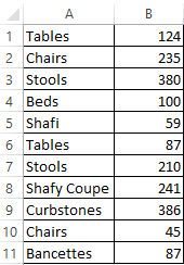
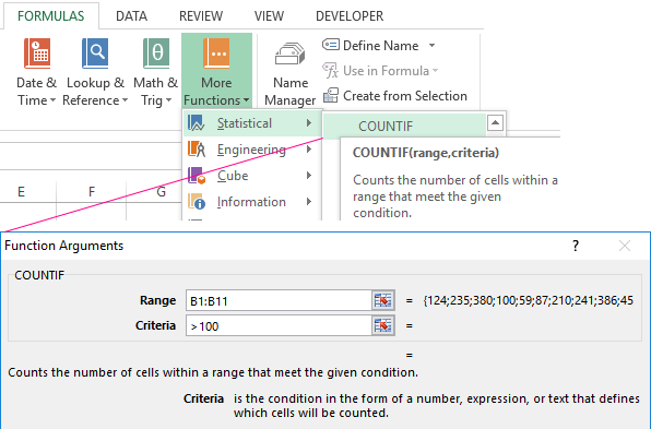
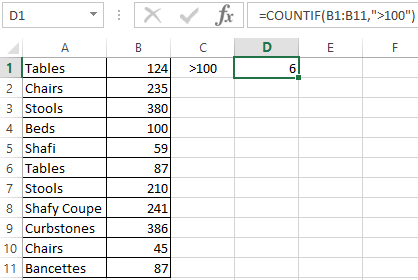
Count the number of cells with numbers greater than 100. Formula: =COUNTIF(B1:B11,»>100″). The range is В1:В11. The counting criterion is «>100». The result:
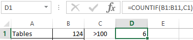
If the counting condition is entered in a separate cell, you can use the reference as a criterion:
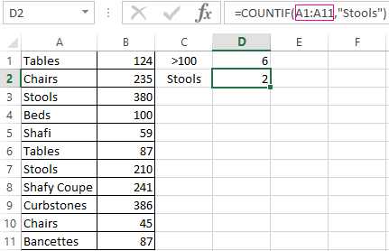
Count the text values in one range. The search condition is one criterion. Formula: =COUNTIF(A1:A11,A3).
Or used reference inside the table:
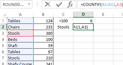
In the second case, the cell reference was used as a criterion, result is the same – 2.
Formula with the wildcard character application: =COUNTIF(A1:A11,»Tab*»). To calculate the number of values ending in «и» and containing any number of characters: =COUNTIF(A1:A11,»*s»). We obtain:
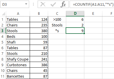
All names that end with a letter «s».
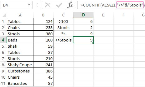
We use the search condition «not equal» in the COUNTIF.
Formula: =COUNTIF(A1:A11,»<>»&»Stools»). The operator «<>» means «not equal». The ampersand sign (&) is used to merge this operator and the “Stools” value.
When you apply a reference, the formula will look like this:
Often you need to perform the COUNTIF function in Excel by two criteria. In this way, you can significantly expand its capabilities. Let’s consider special cases of using the COUNTIF function in Excel and examples with two criteria.
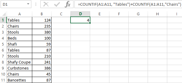
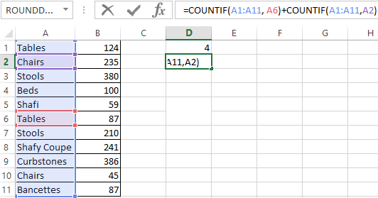
- Let’s count how many cells are contained in the » Tables » and » Chairs » text. Formula:
To specify several criteria, several COUNTIF phrases are used. They are united by the «+» operator.
- Criteria – cell references. Formula:
The function searches for » Tables » text in cell A1 and » Chairs » text – in cell A2 based on the criterion.
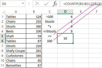
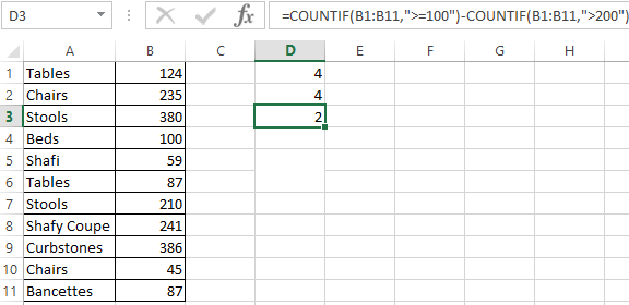
- Count the number of cells in B1:B11 range with a value greater than or equal to 100 and less than or equal to 200. Formula:
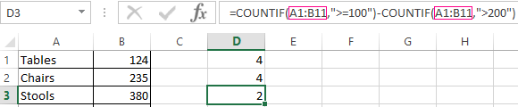
- Apply several ranges in the COUNTIF function. This is possible if the ranges are contiguous. It searches for values by two criteria in two columns simultaneously. If the ranges are not adjacent, then the COUNTIFS function is used.
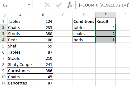
- When the criterion is a reference to a range of cells with conditions, the function returns the array. To enter a formula, you need to highlight as many cells as the range with criteria contains. After entering the arguments, simultaneously press Shift + Ctrl + Enter control key combination. Excel recognizes the formula of the array.
COUNTIF with two criteria in Excel is very often used for automated and efficient data handling. Therefore, an advanced user is highly recommended to carefully study all of the examples above.
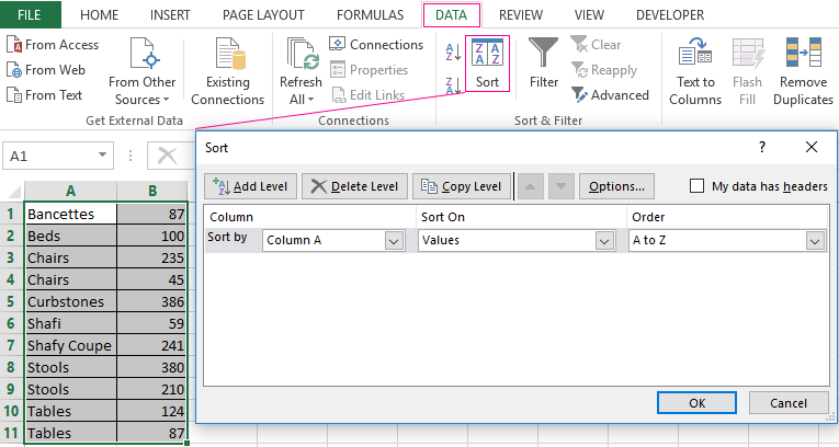
Subtotal command and the countif function
Count the number of goods sold in groups.
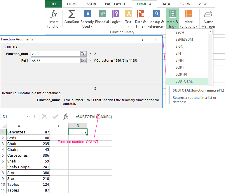
- First, sort the table so that the same values are close.
- The first argument of the formula “SUBTOTAL” – “Function number”. These are numbers from 1 to 11, indicating a statistical function for calculating the intermediate result. Counting the number of cells is carried out under number «2» (“COUNT”).
Download example COUNTIF in Excel
The formula has found the number of values for the «Chairs» group. For a large number of rows (more than a thousand), this combination of functions can be useful.