
Excel for Microsoft 365 Excel 2021 Excel 2019 Excel 2016 Excel 2013 Excel 2010 Excel 2007 More…Less
To count numbers or dates that meet a single condition (such as equal to, greater than, less than, greater than or equal to, or less than or equal to), use the COUNTIF function. To count numbers or dates that fall within a range (such as greater than 9000 and at the same time less than 22500), you can use the COUNTIFS function. Alternately, you can use SUMPRODUCT too.
Example
Note: You’ll need to adjust these cell formula references outlined here based on where and how you copy these examples into the Excel sheet.
|
1 |
A |
B |
|---|---|---|
|
2 |
Salesperson |
Invoice |
|
3 |
Buchanan |
15,000 |
|
4 |
Buchanan |
9,000 |
|
5 |
Suyama |
8,000 |
|
6 |
Suyma |
20,000 |
|
7 |
Buchanan |
5,000 |
|
8 |
Dodsworth |
22,500 |
|
9 |
Formula |
Description (Result) |
|
10 |
=COUNTIF(B2:B7,»>9000″) |
The COUNTIF function counts the number of cells in the range B2:B7 that contain numbers greater than 9000 (4) |
|
11 |
=COUNTIF(B2:B7,»<=9000″) |
The COUNTIF function counts the number of cells in the range B2:B7 that contain numbers less than 9000 (4) |
|
12 |
=COUNTIFS(B2:B7,»>=9000″,B2:B7,»<=22500″) |
The COUNTIFS function (available in Excel 2007 and later) counts the number of cells in the range B2:B7 greater than or equal to 9000 and are less than or equal to 22500 (4) |
|
13 |
=SUMPRODUCT((B2:B7>=9000)*(B2:B7<=22500)) |
The SUMPRODUCT function counts the number of cells in the range B2:B7 that contain numbers greater than or equal to 9000 and less than or equal to 22500 (4). You can use this function in Excel 2003 and earlier, where COUNTIFS is not available. |
|
14 |
Date |
|
|
15 |
3/11/2011 |
|
|
16 |
1/1/2010 |
|
|
17 |
12/31/2010 |
|
|
18 |
6/30/2010 |
|
|
19 |
Formula |
Description (Result) |
|
20 |
=COUNTIF(B14:B17,»>3/1/2010″) |
Counts the number of cells in the range B14:B17 with a data greater than 3/1/2010 (3) |
|
21 |
=COUNTIF(B14:B17,»12/31/2010″) |
Counts the number of cells in the range B14:B17 equal to 12/31/2010 (1). The equal sign is not needed in the criteria, so it is not included here (the formula will work with an equal sign if you do include it («=12/31/2010»). |
|
22 |
=COUNTIFS(B14:B17,»>=1/1/2010″,B14:B17,»<=12/31/2010″) |
Counts the number of cells in the range B14:B17 that are between (inclusive) 1/1/2010 and 12/31/2010 (3). |
|
23 |
=SUMPRODUCT((B14:B17>=DATEVALUE(«1/1/2010»))*(B14:B17<=DATEVALUE(«12/31/2010»))) |
Counts the number of cells in the range B14:B17 that are between (inclusive) 1/1/2010 and 12/31/2010 (3). This example serves as a substitute for the COUNTIFS function that was introduced in Excel 2007. The DATEVALUE function converts the dates to a numeric value, which the SUMPRODUCT function can then work with. |
Need more help?
Want more options?
Explore subscription benefits, browse training courses, learn how to secure your device, and more.
Communities help you ask and answer questions, give feedback, and hear from experts with rich knowledge.
Содержание
- COUNTIFS function
- Syntax
- Remarks
- Example 1
- COUNTIF function
- Examples
- Common Problems
- Best practices
- Need more help?
- COUNTIF Function
- Related functions
- Summary
- Purpose
- Return value
- Arguments
- Syntax
- Usage notes
- Syntax
- Applying criteria
- Blank cells
- Dates
- Wildcards
- OR logic
- Limitations
- COUNTIF with non-contiguous range
- Related functions
- Summary
- Generic formula
- Explanation
- INDIRECT and COUNTIF
- Multiple COUNTIFs
- VSTACK function
COUNTIFS function
The COUNTIFS function applies criteria to cells across multiple ranges and counts the number of times all criteria are met.

This video is part of a training course called Advanced IF functions.
Syntax
COUNTIFS(criteria_range1, criteria1, [criteria_range2, criteria2]…)
The COUNTIFS function syntax has the following arguments:
criteria_range1 Required. The first range in which to evaluate the associated criteria.
criteria1 Required. The criteria in the form of a number, expression, cell reference, or text that define which cells will be counted. For example, criteria can be expressed as 32, «>32», B4, «apples», or «32».
criteria_range2, criteria2, . Optional. Additional ranges and their associated criteria. Up to 127 range/criteria pairs are allowed.
Important: Each additional range must have the same number of rows and columns as the criteria_range1 argument. The ranges do not have to be adjacent to each other.
Each range’s criteria is applied one cell at a time. If all of the first cells meet their associated criteria, the count increases by 1. If all of the second cells meet their associated criteria, the count increases by 1 again, and so on until all of the cells are evaluated.
If the criteria argument is a reference to an empty cell, the COUNTIFS function treats the empty cell as a 0 value.
You can use the wildcard characters— the question mark (?) and asterisk (*) — in criteria. A question mark matches any single character, and an asterisk matches any sequence of characters. If you want to find an actual question mark or asterisk, type a tilde (
) before the character.
Example 1
Copy the example data in the following tables, and paste it in cell A1 of a new Excel worksheet. For formulas to show results, select them, press F2, and then press Enter. If you need to, you can adjust the column widths to see all the data.
Источник
COUNTIF function
Use COUNTIF, one of the statistical functions, to count the number of cells that meet a criterion; for example, to count the number of times a particular city appears in a customer list.
In its simplest form, COUNTIF says:
=COUNTIF(Where do you want to look?, What do you want to look for?)
The group of cells you want to count. Range can contain numbers, arrays, a named range, or references that contain numbers. Blank and text values are ignored.
A number, expression, cell reference, or text string that determines which cells will be counted.
For example, you can use a number like 32, a comparison like «>32», a cell like B4, or a word like «apples».
COUNTIF uses only a single criteria. Use COUNTIFS if you want to use multiple criteria.
Examples
To use these examples in Excel, copy the data in the table below, and paste it in cell A1 of a new worksheet.
Counts the number of cells with apples in cells A2 through A5. The result is 2.
Counts the number of cells with peaches (the value in A4) in cells A2 through A5. The result is 1.
Counts the number of apples (the value in A2), and oranges (the value in A3) in cells A2 through A5. The result is 3. This formula uses COUNTIF twice to specify multiple criteria, one criteria per expression. You could also use the COUNTIFS function.
Counts the number of cells with a value greater than 55 in cells B2 through B5. The result is 2.
Counts the number of cells with a value not equal to 75 in cells B2 through B5. The ampersand (&) merges the comparison operator for not equal to (<>) and the value in B4 to read =COUNTIF(B2:B5,»<>75″). The result is 3.
=COUNTIF(B2:B5,»>=32″)-COUNTIF(B2:B5,» ) or equal to (=) 32 and less than (
Common Problems
What went wrong
Wrong value returned for long strings.
The COUNTIF function returns incorrect results when you use it to match strings longer than 255 characters.
To match strings longer than 255 characters, use the CONCATENATE function or the concatenate operator &. For example, =COUNTIF(A2:A5,»long string»&»another long string»).
No value returned when you expect a value.
Be sure to enclose the criteria argument in quotes.
A COUNTIF formula receives a #VALUE! error when referring to another worksheet.
This error occurs when the formula that contains the function refers to cells or a range in a closed workbook and the cells are calculated. For this feature to work, the other workbook must be open.
Best practices
Be aware that COUNTIF ignores upper and lower case in text strings.
Criteria aren’t case sensitive. In other words, the string «apples» and the string «APPLES» will match the same cells.
Use wildcard characters.
Wildcard characters —the question mark (?) and asterisk (*)—can be used in criteria. A question mark matches any single character. An asterisk matches any sequence of characters. If you want to find an actual question mark or asterisk, type a tilde (
) in front of the character.
For example, =COUNTIF(A2:A5,»apple?») will count all instances of «apple» with a last letter that could vary.
Make sure your data doesn’t contain erroneous characters.
When counting text values, make sure the data doesn’t contain leading spaces, trailing spaces, inconsistent use of straight and curly quotation marks, or nonprinting characters. In these cases, COUNTIF might return an unexpected value.
For convenience, use named ranges
COUNTIF supports named ranges in a formula (such as =COUNTIF( fruit,»>=32″)-COUNTIF( fruit,»>85″). The named range can be in the current worksheet, another worksheet in the same workbook, or from a different workbook. To reference from another workbook, that second workbook also must be open.
Note: The COUNTIF function will not count cells based on cell background or font color. However, Excel supports User-Defined Functions (UDFs) using the Microsoft Visual Basic for Applications (VBA) operations on cells based on background or font color. Here is an example of how you can Count the number of cells with specific cell color by using VBA.
Need more help?
You can always ask an expert in the Excel Tech Community or get support in the Answers community.
Источник
COUNTIF Function
Summary
COUNTIF is an Excel function to count cells in a range that meet a single condition. COUNTIF can be used to count cells that contain dates, numbers, and text. The criteria used in COUNTIF supports logical operators (>, ,=) and wildcards (*,?) for partial matching.
Purpose
Return value
Arguments
- range — The range of cells to count.
- criteria — The criteria that controls which cells should be counted.
Syntax
Usage notes
The COUNTIF function counts cells in a range that meet a given condition, referred to as criteria. COUNTIF is a common, widely used function in Excel, and can be used to count cells that contain dates, numbers, and text. Note that COUNTIF can only apply a single condition. To count cells with multiple criteria, see the COUNTIFS function.
Syntax
The generic syntax for COUNTIF looks like this:
The COUNTIF function takes two arguments, range and criteria. Range is the range of cells to apply a condition to. Criteria is the condition to apply, along with any logical operators that are needed.
Applying criteria
The COUNTIF function supports logical operators (>, , =) and wildcards (*,?) for partial matching. The tricky part about using the COUNTIF function is the syntax used to apply criteria. COUNTIFS is in a group of eight functions that split logical criteria into two parts, range and criteria. Because of this design, each condition requires a separate range and criteria argument, and operators in the criteria must be enclosed in double quotes («»). The table below shows examples of the syntax needed for common criteria:
| Target | Criteria |
|---|---|
| Cells greater than 75 | «>75» |
| Cells equal to 100 | 100 or «100» |
| Cells less than or equal to 100 | » red» |
| Cells that are blank «» | «» |
| Cells that are not blank | «<>« |
| Cells that begin with «X» | «x*» |
| Cells less than A1 | » » operator surrounded by double quotes («»). For example, the formula below will count cells not equal to «red» in the range A1:A10:
Blank cellsCOUNTIF can count cells that are blank or not blank. The formulas below count blank and not blank cells in the range A1:A10: Note: be aware that COUNTIF treats formulas that return an empty string («») as not blank. See this example for some workarounds to this problem. DatesThe easiest way to use COUNTIF with dates is to refer to a valid date in another cell with a cell reference. For example, to count cells in A1:A10 that contain a date greater than the date in B1, you can use a formula like this: Notice we must concatenate an operator to the date in B1. To use more advanced date criteria (i.e. all dates in a given month, or all dates between two dates) you’ll want to switch to the COUNTIFS function, which can handle multiple criteria. The safest way to hardcode a date into COUNTIF is to use the DATE function. This ensures Excel will understand the date. To count cells in A1:A10 that contain a date less than April 1, 2020, you can use a formula like this WildcardsThe wildcard characters question mark (?), asterisk(*), or tilde ( ) can be used in criteria. A question mark (?) matches any one character and an asterisk (*) matches zero or more characters of any kind. For example, to count cells in A1:A5 that contain the text «apple» anywhere, you can use a formula like this: To count cells in A1:A5 that contain any 3 text characters, you can use: ) is an escape character to match literal wildcards. For example, to count a literal question mark (?), asterisk(*), or tilde ( ), add a tilde in front of the wildcard (i.e. OR logicThe COUNTIF function is designed to apply just one condition. However, to count cells that contain «this OR that», you can use an array constant and the SUM function like this: The formula above will count cells in range that contain «red» or «blue». Essentially, COUNTIF returns two counts in an array (one for «red» and one for «blue») and the SUM function returns the sum. For more information, see this example. LimitationsThe COUNTIF function has some limitations you should be aware of:
The most common way to work around the limitations above is to use the SUMPRODUCT function. In the current version of Excel, another option is to use the newer BYROW and BYCOL functions. Источник COUNTIF with non-contiguous range
SummaryTo count values in separate ranges with criteria, you can use the COUNTIF function together with INDIRECT and SUM. In the example shown, cell I5 contains this formula: The result is 9, since there are nine values greater than 50 in the three ranges shown. Note: In Excel 365, the VSTACK and HSTACK functions offer a new approach to this problem. See below for an example. Generic formulaExplanationIn this example, the goal is to count values in three non-contiguous ranges with criteria. To be included in the count, values must be greater than 50. The COUNTIF counts the number of cells in a range that meet given criteria. However, COUNTIF does not perform counts across different ranges. If you try to use COUNTIF with multiple ranges separated by commas, or in an array constant, you’ll get an error. There are several ways to approach this problem, as explained below. INDIRECT and COUNTIFThe INDIRECT function converts a given text string into a proper Excel reference: One approach is to provide the ranges as text in an array constant to INDIRECT like this: Then pass the result from INDIRECT into the COUNTIF function like this: INDIRECT will evaluate the text values and pass the references into COUNTIF as the range argument. For reasons mysterious, COUNTIF will accept the result from INDIRECT without complaint. Because COUNTIF receives more than one range, it will return more than one result in an array like this: The three numbers in this array are the counts of numbers greater than 50 in each of the three ranges. To «catch» these results and return a total, we use the SUM function: The SUM function then returns the sum of all values, 9. Although this is an array formula, it does not require CSE, since we are using an array constant. Note: INDIRECT is a volatile function and can impact workbook performance. Multiple COUNTIFsAnother way to solve this problem is to use more than one COUNTIF: With a limited number of ranges, this approach may be easier to implement. It avoids possible performance impacts of INDIRECT, and allows a normal formula syntax for ranges, so ranges will update automatically with worksheet changes. The INDIRECT example above relies on text strings that need to be updated manually. VSTACK functionIn current versions of Excel, a better approach is to first combine the ranges, then perform the conditional count. To combine all three ranges vertically, you can use the VSTACK function: The result from VSTACK is a single array with 14 values. Unfortunately, we can’t pass this result into the COUNTIF function, because COUNTIF is in a group of functions that require actual ranges. However, we can use the SUM function and Boolean algebra to perform the conditional count. The complete formula looks like this: After VSTACK runs, and all values are checked with >50, we have an array of 14 TRUE and FALSE values like this: The double negative (—) is used to convert the TRUE and FALSE values to 1s and 0s, and the resulting array is returned directly to the SUM function: The SUM function sums the array and returns 9 as a final result. Источник Adblock |

Return to Excel Formulas List
Download Example Workbook
Download the example workbook
This tutorial explains how to count the number of cells containing numbers that fall within a specified range using the COUNTIFS function.
COUNTIFS
COUNTIFS(range_1,criteria _1,[ range_2,criteria _2],…)
- range_1 (required): group of cells to count
- criteria_1 (required): conditions used to count
- range_2,criteria_2: optional ranges and criteria than can be evaluated. Up to 127 range and criteria pairs can be specified.
How COUNTIFS Works
The COUNTIFS function adds up the number of cells that fall within the ranges specified in the COUNTIF Function.
Let us see how to actually use the function. The following image shows COUNTIFS in action.
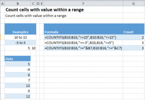
COUNTIFS Cells in Range Example Description
Let us now look at the formula and try to understand it, piece by piece.
- In the first case, we call COUNTIFS in the following manner: =COUNTIFS(B10:B16,”>=10”,B10:B16 ,”<=15”)
- B10:B16 tells Excel the range over which we want to count
- “>=10”/ “<=15”, the criteria according to which we want to count the cells.
- “>=10″ stands for counting any value that is greater than or equal to 10
- “<=15” stands for counting any value that is less than or equal to 15
- The second case is similar to the first case with only the counting criteria changing to
- “>=5”, greater than or equal to -5, i.e. -4,- 3, -2, -1, 0, 1…
- “<=5”, less than or equal to 5
- The third case is a special case, one which we are very likely to face in a real life situation. This example shows us how to pick values like 5 and 10 from the spreadsheet rather than manually writing them in the formula. To achieve this, we call our function in the following manner: =COUNTIFS(B10:B16,”>=”&B7,B10:B16 ,”<=”&C7)
- The only thing changed in our function call as compared to before is our way of providing it our criterion, “>=”&B7/ “<=”&C7. The & sign followed by a cell number tells Excel to look at the value contained in the mentioned cell and use it to substitute it in the formula. Hence,
- The &B7 in “>=”&B7, tells excel to look for the value in the cell B7, which in our case is 5, and substitute it in our formula changing it into “>=5”
- Similarly &C7 in “<=”&C7 is translated by excel into “<=10”
- The only thing changed in our function call as compared to before is our way of providing it our criterion, “>=”&B7/ “<=”&C7. The & sign followed by a cell number tells Excel to look at the value contained in the mentioned cell and use it to substitute it in the formula. Hence,
COUNTIF Function
Before ending this tutorial, I would also like to talk a bit about the COUNTIF function.
Like COUNTIFS, COUNTIF can also be used to count the number of cells meeting specific criteria, but with one very important difference.
The difference between the COUNTIF and COUNTIFS functions is that while the latter function can be used to match multiple criteria in multiple ranges, the former can only match a single criterion in a single range. Multiple COUNTIF calls will be required to achieve this result.
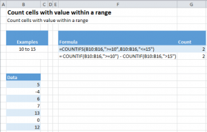
The image below shows how to find the count for the first case in above example using COUNTIF function:
EXPLANATION
The COUNTIF function is called as below:
= COUNTIF(B10:B16,”>=10″) – COUNTIF(B10:B16,”>15″)
The “>15” means all values greater than 15 will be counted but not 15 itself.
There are 3 operations happening over here
- The first COUNTIF is counting all the values which are greater than or equal to 10
- The second COUNTIF is counting all values that are strictly greater than 15
- The final operation is subtracting the two counts found above in order to find our final count
The COUNTIF function counts cells in a range that meet a given condition, referred to as criteria. COUNTIF is a common, widely used function in Excel, and can be used to count cells that contain dates, numbers, and text. Note that COUNTIF can only apply a single condition. To count cells with multiple criteria, see the COUNTIFS function.
Syntax
The generic syntax for COUNTIF looks like this:
=COUNTIF(range,criteria)The COUNTIF function takes two arguments, range and criteria. Range is the range of cells to apply a condition to. Criteria is the condition to apply, along with any logical operators that are needed.
Applying criteria
The COUNTIF function supports logical operators (>,<,<>,<=,>=) and wildcards (*,?) for partial matching. The tricky part about using the COUNTIF function is the syntax used to apply criteria. COUNTIFS is in a group of eight functions that split logical criteria into two parts, range and criteria. Because of this design, each condition requires a separate range and criteria argument, and operators in the criteria must be enclosed in double quotes («»). The table below shows examples of the syntax needed for common criteria:
| Target | Criteria |
|---|---|
| Cells greater than 75 | «>75» |
| Cells equal to 100 | 100 or «100» |
| Cells less than or equal to 100 | «<=100» |
| Cells equal to «Red» | «red» |
| Cells not equal to «Red» | «<>red» |
| Cells that are blank «» | «» |
| Cells that are not blank | «<>» |
| Cells that begin with «X» | «x*» |
| Cells less than A1 | «<«&A1 |
| Cells less than today | «<«&TODAY() |
Notice the last two examples involve concatenation with the ampersand (&) character. Any time you are using a value from another cell, or using the result of a formula in criteria with a logical operator like «<«, you will need to concatenate. This is because Excel needs to evaluate cell references and formulas first to get a value, before that value can be joined to an operator.
Basic example
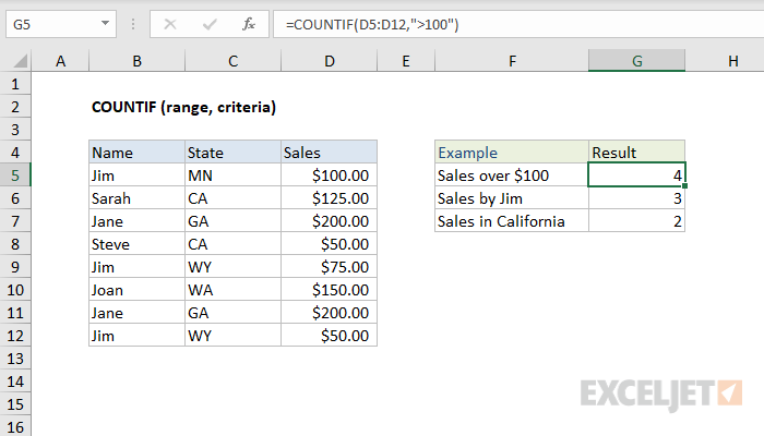
In the worksheet shown above, the following formulas are used in cells G5, G6, and G7:
=COUNTIF(D5:D12,">100") // count sales over 100
=COUNTIF(B5:B12,"jim") // count name = "jim"
=COUNTIF(C5:C12,"ca") // count state = "ca"
Notice COUNTIF is not case-sensitive, «CA» and «ca» are treated the same.
Double quotes («») in criteria
In general, text values need to be enclosed in double quotes («»), and numbers do not. However, when a logical operator is included with a number, the number and operator must be enclosed in quotes, as seen in the second example below:
=COUNTIF(A1:A10,100) // count cells equal to 100
=COUNTIF(A1:A10,">32") // count cells greater than 32
=COUNTIF(A1:A10,"jim") // count cells equal to "jim"
Value from another cell
A value from another cell can be included in criteria using concatenation. In the example below, COUNTIF will return the count of values in A1:A10 that are less than the value in cell B1. Notice the less than operator (which is text) is enclosed in quotes.
=COUNTIF(A1:A10,"<"&B1) // count cells less than B1
Not equal to
To construct «not equal to» criteria, use the «<>» operator surrounded by double quotes («»). For example, the formula below will count cells not equal to «red» in the range A1:A10:
=COUNTIF(A1:A10,"<>red") // not "red"
Blank cells
COUNTIF can count cells that are blank or not blank. The formulas below count blank and not blank cells in the range A1:A10:
=COUNTIF(A1:A10,"<>") // not blank
=COUNTIF(A1:A10,"") // blank
Note: be aware that COUNTIF treats formulas that return an empty string («») as not blank. See this example for some workarounds to this problem.
Dates
The easiest way to use COUNTIF with dates is to refer to a valid date in another cell with a cell reference. For example, to count cells in A1:A10 that contain a date greater than the date in B1, you can use a formula like this:
=COUNTIF(A1:A10, ">"&B1) // count dates greater than A1
Notice we must concatenate an operator to the date in B1. To use more advanced date criteria (i.e. all dates in a given month, or all dates between two dates) you’ll want to switch to the COUNTIFS function, which can handle multiple criteria.
The safest way to hardcode a date into COUNTIF is to use the DATE function. This ensures Excel will understand the date. To count cells in A1:A10 that contain a date less than April 1, 2020, you can use a formula like this
=COUNTIF(A1:A10,"<"&DATE(2020,4,1)) // dates less than 1-Apr-2020
Wildcards
The wildcard characters question mark (?), asterisk(*), or tilde (~) can be used in criteria. A question mark (?) matches any one character and an asterisk (*) matches zero or more characters of any kind. For example, to count cells in A1:A5 that contain the text «apple» anywhere, you can use a formula like this:
=COUNTIF(A1:A5,"*apple*") // cells that contain "apple"
To count cells in A1:A5 that contain any 3 text characters, you can use:
=COUNTIF(A1:A5,"???") // cells that contain any 3 characters
The tilde (~) is an escape character to match literal wildcards. For example, to count a literal question mark (?), asterisk(*), or tilde (~), add a tilde in front of the wildcard (i.e. ~?, ~*, ~~).
OR logic
The COUNTIF function is designed to apply just one condition. However, to count cells that contain «this OR that», you can use an array constant and the SUM function like this:
=SUM(COUNTIF(range,{"red","blue"})) // red or blue
The formula above will count cells in range that contain «red» or «blue». Essentially, COUNTIF returns two counts in an array (one for «red» and one for «blue») and the SUM function returns the sum. For more information, see this example.
Limitations
The COUNTIF function has some limitations you should be aware of:
- COUNTIF only supports a single condition. If you need to count cells using multiple criteria, use the COUNTIFS function.
- COUNTIF requires an actual range for the range argument; you can’t provide an array. This means you can’t alter values in range before applying criteria.
- COUNTIF is not case-sensitive. Use the EXACT function for case-sensitive counts.
- COUNTIFS has other quirks explained in this article.
The most common way to work around the limitations above is to use the SUMPRODUCT function. In the current version of Excel, another option is to use the newer BYROW and BYCOL functions.
Notes
- Text strings in criteria must be enclosed in double quotes («»), i.e. «apple», «>32», «app*»
- Cell references in criteria are not enclosed in quotes, i.e. «<«&A1
- The wildcard characters ? and * can be used in criteria. A question mark matches any one character and an asterisk matches any sequence of characters (zero or more).
- To match a literal question mark(?) or asterisk (*), use a tilde (~) like (~?, ~*).
- COUNTIF requires a range, you can’t substitute an array.
- COUNTIF returns incorrect results when used to match strings longer than 255 characters.
- COUNTIF will return a #VALUE error when referencing another workbook that is closed.
Here is a COUNTIF function with an additional range of values to match at the end. Why does it not work and how can I get it to work.
=COUNTIF('[DATABASE 1.xlsx]Sheet1'!$AC$3:$AC$51877,AND('[DATABASE 1.xlsx]Sheet1'!$AC$3:$AC$51877>=548,'[DATABASE 1.xlsx]Sheet1'!$AC$3:$AC$51877<=554)
asked Mar 30, 2012 at 15:49
![]()
If you can’t use COUNTIFS you subtract one COUNTIF from another like this
=COUNTIF('[DATABASE 1.xlsx]Sheet1'!$AC$3:$AC$51877,">=548")-COUNTIF('[DATABASE 1.xlsx]Sheet1'!$AC$3:$AC$51877,">554")
that counts between 548 and 554 inclusive
answered Mar 30, 2012 at 18:01
![]()
barry houdinibarry houdini
45.5k8 gold badges63 silver badges80 bronze badges
1
You cannot use COUNTIF with AND because the second part must be a criteria.
Plus, the second part (criteria) shouldn’t repeat the range.
You can use COUNTIFS if you are using Excel version 2007 or higher. Else, you can use an array formula.
Something like this maybe:
=COUNTIFS('[DATABASE 1.xlsx]Sheet1'!$AC$3:$AC$51877,">=548",
          '[DATABASE 1.xlsx]Sheet1'!$AC$3:$AC$51877,"<=554")
answered Mar 30, 2012 at 16:14
![]()
JMaxJMax
25.9k12 gold badges69 silver badges88 bronze badges
In this article, we will learn how to Check values which start with either A, B or C using wildcards in Excel.
In simple words, while working with table values, sometimes we need to check the value in cell whether it starts with A, B or C. Example if we need to find the check of a certain ID value starts with either A, B or C. Criteria inside the formula executed using the operators.
How to solve the problem ?
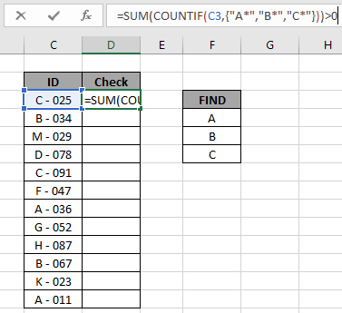
For this article we will be required to use the COUNTIF function. Now we will make a formula out of the function. Here we are given some values in a range and specific text value as criteria. We need to count the values where the formula checks for the value which starts with either A, B or C.
Generic formula:
= SUM ( COUNTIF ( cell value, { «A*» , «B*» , «C*» } ) ) > 0
Cell value : value where condition is checked.
* : wildcards which find any number of characters within a given cell.
A* : given text or pattern to look for. Use pattern directly in the formula or else if you using cell reference for the pattern use the other formula shown below.
Example:
All of these might be confusing to understand. So, let’s test this formula via running it on the example shown below.
Here we have the ID records and we need to find the IDs which starts with either A, B or C.
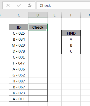
Here to find the category IDs which starts with either A , B or C, will be using the * (asterisk) wildcard in the formula. * (asterisk) wildcard finds any number of characters within lookup value.
Use the formula:
= SUM ( COUNTIF ( C3 , { «A*» , «B*» , «C*» } ) ) >0
Explanation:
- COUNTIF function checks the value which matches with either of the pattern stated in the formula
- Criteria is given in using * (asterisk) wildcard to look for value which has any number of characters.
- COUNTIF function returns an array to the SUM function matching either of the values.
- SUM function adds up all the values and checks whether the sum comes out to be greater than 0 or not.
Here the range is given as array reference and pattern is given as cell reference. Press Enter to get the count.
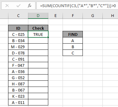
As you can see the formula returns TRUE for the value in C3 cell. Now copy the formula in other cells using the drag down option or using the shortcut key Ctrl + D as shown below.
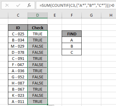
As you can see all the TRUE values indicate the cell value starts with either of mentioned pattern and all the FALSE values states there is the cell value starts with neither of mentioned pattern.
Verification:
You can check which values start with a specific pattern in range using the excel filter option. Apply the filter to the ID header and click the arrow button which appears. Follow the steps as shown below.
Steps:
- Select the ID header cell. Apply filter using shortcut Ctrl + Shift + L
- Click the arrow which appeared as a filter option.
- Deselect (Select All) option.
- Now search in search box using the * (asterisk) wildcard.
- Type A* in the search box and select the required values or select the (Select All search result) option as shown in the above gif.
- Do it for the other two values and get the count of all three which is equal to the result returned by the formula.
As you can see in the above gif all the 6 values which match the given pattern. This also means the formula works fine to get to check the values
Here are some observational notes shown below.
Notes:
- The formula only works with numbers and text both
- Operators like equals to ( = ), less than equal to ( <= ), greater than ( > ) or not equals to ( <> ) can be performed within function applied with numbers only.
Hope this article about how to Check values which start with either A , B or C using wildcards in Excel is explanatory. Find more articles on COUNTIF functions here. If you liked our blogs, share it with your fristarts on Facebook. And also you can follow us on Twitter and Facebook. We would love to hear from you, do let us know how we can improve, complement or innovate our work and make it better for you. Write us at info@exceltip.com
Related Articles
How to use the SUMPRODUCT function in Excel: Returns the SUM after multiplication of values in multiple arrays in excel.
COUNTIFS with Dynamic Criteria Range : Count cells depstartent on other cell values in Excel.
COUNTIFS Two Criteria Match : Count cells matching two different criteria on list in excel.
COUNTIFS With OR For Multiple Criteria : Count cells having multiple criteria match using the OR function.
The COUNTIFS Function in Excel : Count cells dependent on other cell values.
How to Use Countif in VBA in Microsoft Excel : Count cells using Visual Basic for Applications code.
How to use wildcards in excel : Count cells matching phrases using the wildcards in excel
Popular Articles
50 Excel Shortcut to Increase Your Productivity : Get faster at your task. These 50 shortcuts will make you work even faster on Excel.
How to use the VLOOKUP Function in Excel : This is one of the most used and popular functions of excel that is used to lookup value from different ranges and sheets.
How to use the COUNTIF function in Excel : Count values with conditions using this amazing function. You don’t need to filter your data to count specific values. Countif function is essential to prepare your dashboard.
How to Use SUMIF Function in Excel : This is another dashboard essential function. This helps you sum up values on specific conditions.
The COUNTIF function in Excel counts the number of cells within a range based on pre-defined criteria. It is used to count cells that include dates, numbers, or text. For example, COUNTIF(A1:A10,”Trump”) will count the number of cells within the range A1:A10 that contain the text “Trump”
Syntax
The syntax of COUNTIF formula in Excel is stated as follows:
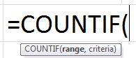
It accepts the following required arguments:
- Range: It represents the range of values on which the criteria will be applied.
- Criteria: It represents the condition that is applied to the range of values. The values that meet the criteria are returned as a result.
The output of the COUNTIF formula is a positive number which can be zero or non-zero.
Table of contents
- What is COUNTIF Function in Excel
- Syntax
- How to Use COUNTIF Function in Excel?
- #1 – Count Values with the Given Value
- #2 – Count Numbers with a Value Less Than the Given Number
- #3 – Count Values with the Given Text Value
- #4 – Count Negative Numbers
- #5 – Count Zero Values
- The Criteria of the COUNTIF Formula
- Frequently Asked Questions (FAQs)
- Video
- Recommended Articles
How to Use COUNTIF Function in Excel?
Being a worksheet (WS) function, the COUNTIF function can be entered as a part of the cell formula. The usage of the COUNTIF function is the same in Excel and VBA (COUNTIF function VBAVBA COUNTIF is a worksheet function used to count the number of times the criteria are fulfilled in the worksheet range. The VBA code for this function is written as WorksheetFunction.CountIf.read more).
You can download this COUNTIF Function Excel Template here – COUNTIF Function Excel Template
Let us consider some uses to understand the working of the COUNTIF excel function.
#1 – Count Values with the Given Value
The following table shows a list containing numerical values in the cells A2:A7. Count the given range of cells for the values matching the number “33”.
The COUNTIF function is applied to the given range of cells, and the formula is stated as follows:
“=COUNTIF (A2:A7,33)”
Here the condition applied to the formula is the number “33”.The formula checks the range of cells A2:A7 for the values matching number “33”. The range contains only one such number, which satisfies the condition. Hence the result returned by the COUNTIF function is “1”. The result is displayed in cell A8.

#2 – Count Numbers with a Value Less Than the Given Number
A list of data in the cells A12:A17 is provided in the succeeding table. Count the given range of cells for the values less than “50”.
The COUNTIF function is applied to the given range of cells, and the formula is stated as follows:
“=COUNTIF(A12:A17,“<50”)”
Here the condition applied to the formula is “<50”. The COUNTIF formula checks the range of cells matching the condition, less than 50. There are only four values that are less than 50 in the range. Hence the result returned by this function is “4”. The result is displayed in cell A18.

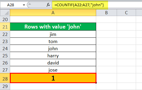
#3 – Count Values with the Given Text Value
A list of data in the cells A22:A27 is provided in the below table. Count the range of cells for the text value “john”.
The COUNTIF function is applied to the given range of cells, and the formula is stated as follows:
“=COUNTIF(A22:A27, “john”)”
Here the condition applied to the formula is the value “john.” The COUNTIF formula checks the range of cells matching the given condition. The given range has only one cell that satisfies the text value “john”. Hence, the result is “1” which is displayed in cell A28.
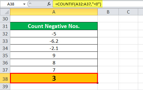
#4 – Count Negative Numbers
A list of data in the range of cells A32:A37 is provided in the below table. Count the range of cells for negative values (that is, less than zero).
The COUNTIF function is applied to the given range of cells, and the formula is stated as follows:
“=COUNTIF(A32:A37, “<0”)”
Here the condition applied to the formula is less than zero. Now, the COUNTIF formula will identify and count the numbers with negative values in the given range. There are three such numbers in the given range. Hence, the result is “3” which is displayed in cell A38.
#5 – Count Zero Values
A list of data in the range of cells A42:A47 is provided in the below table. Count the range of cells for the value “0”.
The COUNTIF function is applied to the given range of cells, and the formula is stated as follows:
“=COUNTIF(A42:A47,0)”
Here the condition applied to the formula is equal to “0”. Now the COUNTIF formula will identify and count the numbers with zero values. There are two zeros in the range. Hence, the result returned is “2” which is displayed in cell A48.

The Criteria of the COUNTIF Formula
It is enclosed within double quotes if non-numeric and without quotes if numeric.
It returns the result only if the values in the cell range satisfy the given criteria.
It can be supplied with wildcard characters like “*” and “?”. The question mark matches any one of the characters, and the asterisk matches any sequence of characters.
It uses the tilde operators followed by the wildcard characters such as “~?” and “~*”.
Frequently Asked Questions (FAQs)
1. What is the COUNTIF function in Excel?
COUNTIF function allows counting of the range of cells that meets the specified criteria. It is used to count cells that contain dates, numbers, and text.
The formula is stated as follows:
“=COUNTIF(range,criteria)”
Where,
• “Range” is a required parameter that refers to the range on which the criteria will be applied.
• “Criteria” is another required parameter that represents the condition applied to the values of the range.
2. What is the syntax of the COUNTIF function in Excel for multiple criteria?
The syntax of COUNTIF function for the same range of cells (“range 1”) with multiple criteria (“criteria 1”, “criteria 2”) is as follows:
“=COUNTIF(range 1,criteria 1)+COUNTIF(range 1,criteria 2)”
In the case of counting multiple ranges of cells with multiple criteria, the COUNTIFS function can be used.
3. What is the COUNTIFS function?
COUNTIFS function is used to evaluate cells across multiple ranges, based on single or multiple conditions. It is similar to the COUNTIF, but multiple criteria are used in the formula.
The formula of the COUNTIFS is stated as follows:
“=COUNTIFS(range 1, criteria1, range 2, criteria 2… )”
Where,
• “Range” refers to the given range of cells.
• “Criteria” refers to the conditions applied to the range.
Video
Recommended Articles
This has been a guide to the COUNTIF function in Excel. In this article, we have discussed how to use COUNTIF formula along with case studies and downloadable templates. You may also look at the below useful functions in Excel –
- How to Use Countif not Blank in Excel?The COUNTIF not blank function counts non-blank cells within a range. read more
- Count Unique Values in ExcelIn Excel, there are two ways to count values: 1) using the Sum and Countif function, and 2) using the SUMPRODUCT and Countif function.read more
- How to use FIND in Excel?Find function in excel finds the location of a character or a substring in a text string. In other words it finds the occurrence of a text in another text, as it gives us the position, the output returned by this function is an integer.read more
- COUNT in Excel
The COUNTIF function is included in the group of statistical functions. It allows you to find the number of cells by a certain criterion. The COUNTIF function works with numeric and text values, as well as with dates.
Syntax and features of the function
First, let’s consider the arguments:
- Range – the group of values for analysis and counting (required).
- Criteria – the condition by which cells are to be counted (required).
The range of cells can include textual and numerical values, dates, arrays, and references to numbers. The function ignores empty cells.
A criterion can be a reference, a number, a text string, or an expression. The COUNTIF function only works with one criterion (by default). However, you can “force” it to analyze two criteria simultaneously.
Recommendations for the correct operation of the function:
- If the COUNTIF function refers to a range in another workbook, this workbook must be opened.
- The «Criteria» argument must be enclosed in quotation marks (except for references).
- The function does not take into account the letter case.
- When formulating a counting condition, you can use wildcard characters. The question mark «?» is any character. The asterisk «*» is any sequence of characters. For the formula to search for these signs directly, put a tilde (~) before them.
- For normal operation of the formula, cells with text values should not contain spaces or non-printable characters.
Countif function in Excel: examples
Let’s count the numerical values in one range. The counting condition is one criterion.
We have the following table:
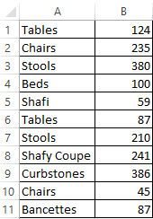
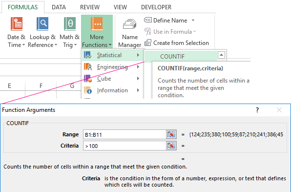
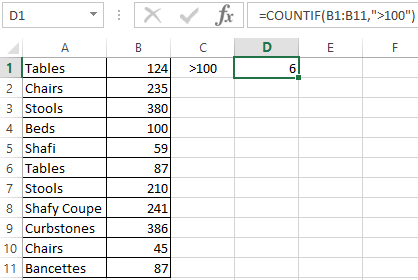
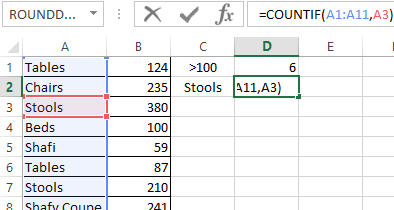
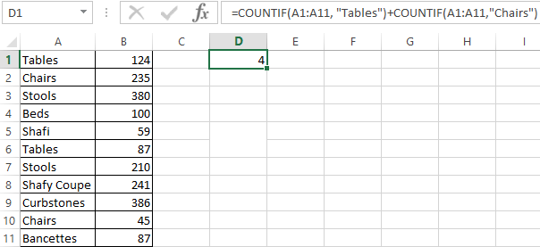
Count the number of cells with numbers greater than 100. Formula: =COUNTIF(B1:B11,»>100″). The range is В1:В11. The counting criterion is «>100». The result:
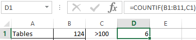
If the counting condition is entered in a separate cell, you can use the reference as a criterion:
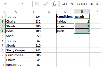
Count the text values in one range. The search condition is one criterion. Formula: =COUNTIF(A1:A11,A3).
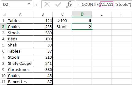
Or used reference inside the table:
In the second case, the cell reference was used as a criterion, result is the same – 2.
Formula with the wildcard character application: =COUNTIF(A1:A11,»Tab*»). To calculate the number of values ending in «и» and containing any number of characters: =COUNTIF(A1:A11,»*s»). We obtain:
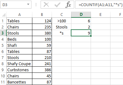
All names that end with a letter «s».
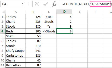
We use the search condition «not equal» in the COUNTIF.
Formula: =COUNTIF(A1:A11,»<>»&»Stools»). The operator «<>» means «not equal». The ampersand sign (&) is used to merge this operator and the “Stools” value.
When you apply a reference, the formula will look like this:
Often you need to perform the COUNTIF function in Excel by two criteria. In this way, you can significantly expand its capabilities. Let’s consider special cases of using the COUNTIF function in Excel and examples with two criteria.
- Let’s count how many cells are contained in the » Tables » and » Chairs » text. Formula:
To specify several criteria, several COUNTIF phrases are used. They are united by the «+» operator.
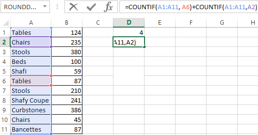
- Criteria – cell references. Formula:
The function searches for » Tables » text in cell A1 and » Chairs » text – in cell A2 based on the criterion.
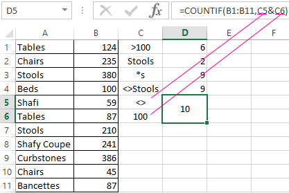
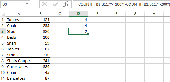
- Count the number of cells in B1:B11 range with a value greater than or equal to 100 and less than or equal to 200. Formula:
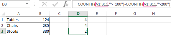
- Apply several ranges in the COUNTIF function. This is possible if the ranges are contiguous. It searches for values by two criteria in two columns simultaneously. If the ranges are not adjacent, then the COUNTIFS function is used.
- When the criterion is a reference to a range of cells with conditions, the function returns the array. To enter a formula, you need to highlight as many cells as the range with criteria contains. After entering the arguments, simultaneously press Shift + Ctrl + Enter control key combination. Excel recognizes the formula of the array.
COUNTIF with two criteria in Excel is very often used for automated and efficient data handling. Therefore, an advanced user is highly recommended to carefully study all of the examples above.
Subtotal command and the countif function
Count the number of goods sold in groups.
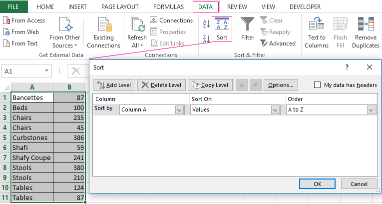
- First, sort the table so that the same values are close.
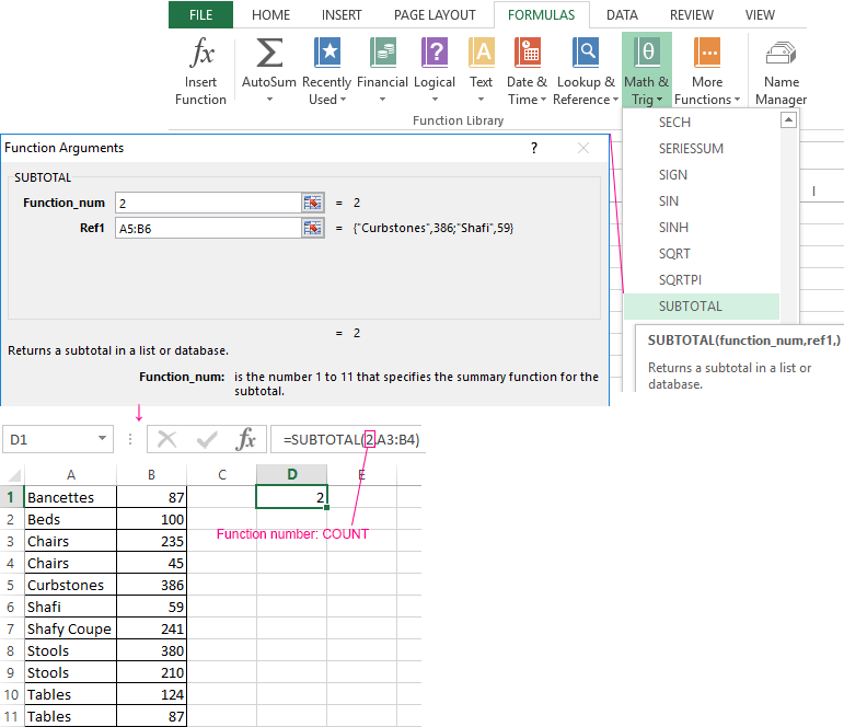
- The first argument of the formula “SUBTOTAL” – “Function number”. These are numbers from 1 to 11, indicating a statistical function for calculating the intermediate result. Counting the number of cells is carried out under number «2» (“COUNT”).
Download example COUNTIF in Excel
The formula has found the number of values for the «Chairs» group. For a large number of rows (more than a thousand), this combination of functions can be useful.
As the name suggests Excel COUNTIF Function is a combination of Count and IF formula. In plain English, COUNTIF Function can be described as a formula that can be used for counting the number of cells that fulfill a particular condition, within a predefined range.
How Excel Defines COUNTIF Function
Microsoft Excel defines COUNTIF as a formula that, “Counts the number of cells within a range that meet the given condition”.
This definition clearly explains that: COUNTIF Function is a better and sophisticated type of COUNT formula that gives you control over, which cells you wish to count.
Syntax of Excel COUNTIF Formula
Excel COUNTIF formula can be written as follows:
=COUNTIF(range , criteria)
Here ‘range’ specifies the range of cells over which you want to apply the ‘criteria‘.
‘criteria’ specifies the condition that a particular cell content should meet to be counted.
How to Use COUNTIF in Excel
Now, let’s see how to use the COUNTIF function in Excel.
Let’s consider, we have an Employee table as shown in the below image.

Objective: From the above table, our objective is to find the number of employees who have joined before 1990.
So, we will try to use the COUNTIF Formula to find the result.

range: In this case, ‘range’ will be “B2:B11”, as on these cells we have to apply the ‘criteria’.

criteria: In this case, ‘ criteria’ is “<01/01/1990”. This specifies that we want to count only those employees that are joined before 1st January 1990.

This results in 6, which means there are 6 employees that have joined before 1990.
Few Important Facts About the COUNTIF Formula
1. COUNTIF formula only accepts a solid range, you cannot give multiple broken ranges to it. For example, COUNTIF cannot be written as
=COUNTIF(A1:A4 , A6:A8, ">0") //This is wrong
=COUNTIF(A1:A8, ">0") //This is correct
2. COUNTIF can accept wildcard characters (like “*” and “?”) in the ‘criteria’ argument. This means that you can write a COUNTIF as
=COUNTIF(D1:D15, "*o*")
This will count all the cells containing the “o” character, within the D1:D5 range.
3. As you know, the output of COUNTIF is an integer so you can also add two COUNTIF functions. For example: if you want to find the cells with value as “1” and cells with value as “2”, so you can use COUNTIF as
=COUNTIF(A1:A10,"1")+COUNTIF(A1:A10,"2")
4. COUNTIF throws a #NAME? error, if you supply an incorrect range to it.
Few Basic Examples of COUNTIF Function

In the above image, I have used an Employee table to depict how the COUNTIF function can be used.
Example 1: In the first example, I have used the Excel COUNTIF formula for finding the number of employees whose first name starts with “G”.
For this, I have used formula as
=COUNTIF(A3:A12,"G*")
Here, the COUNTIF Function scans the whole range from A3:A12 and tries to find a pattern “G*” (‘*’ is a wildcard operator which denotes any number of characters). The resultant is 2, as there are only two persons in the specified range whose first name starts with G.
Example 2: In the second example, I have used a COUNTIF function to find the cells which contain an Employee ID value greater than “26000”.
To accomplish this I have used a formula
=COUNTIF(C3:C12,">26000")
This formula searches the specified range for a value that specifies the criteria (i.e. >26000). So, the result is 5 as only 5 employees have an Employee ID greater than 26000.
Example 3: In the third example, I have fetched the number of employees whose salary is less than 4000.
To get this, I have again used a COUNTIF formula as
=COUNTIF(D3:D12,"<4000")
So, here the COUNTIF counts only those cells where salary range i.e. D3:D12 has a value less than 4000 and the resultant is 3.
Example 4: In the fourth example, I have used the following formula
=COUNTIF(B3:B12,B5)
This formula finds the number of cells equal to the value of the cell B5 (i.e. “Massiot”), in the range B3:B15.
Here, first, the COUNTIF function finds the value at the B5 cell, and then it compares all the cells within the specified range with this value.
The resultant is 2 as only two records match the value at the B5 cell.

Example 5: In the above example, I had to find the total count of cells that contain “Apple” or “Peach”.
This can be easily done by adding the resultants of two COUNTIF statements like:
=COUNTIF(A2:A7,"Apple")+COUNTIF(A2:A7,"Peach")
The first COUNTIF statement gives the number of cells with a value equal to “Apple” and the second statement gives the count of cells with “Peach”. And hence the output comes out as 2+1=3.
Example 6: In this example (i.e. =COUNTIF(A,"Pear")), I have tried to show you what happens if you enter an incorrect range in the COUNTIF function.
In such cases, it throws a #NAME? error.
Few Advanced Examples of COUNTIF Function
Now, let’s see some practical examples of COUNTIF Function.
Example 7: Finding duplicate values using the COUNTIF function.
Let’s say we have a table as below, and we have to find the duplicate records in it.

For finding the duplicate records, we have used the formula:
=COUNTIF($A$2:$A$16,A2)>1
When this formula encounters a duplicate record it returns TRUE, while FALSE means that the record is Unique.

If you are wondering what these dollar ($) signs are doing in this formula, then you should read this post.
Recommended Reading: Find and Delete Duplicate cells in Excel
Example 8: Use the COUNTIF formula for generating the sorting order of a list.
Let’s consider we have a list as below.

Now, If we just want to know the alphabetic sorting order (in ascending order) of the employee names, then we can use the formula:
=COUNTIF($A$2:$A$15,"<="&A2)
See the below image, to see this formula in action.

As you can see, that this formula generates a number in-front of every employee. This number is the sorting order (in ascending sort) of the Employee Names.
Recommended Reading: How to alphabetize a list in Excel
So, this was all from my side. Do share your ideas and experiences related to Excel COUNTIF Function in the below comments section.