
Excel for Microsoft 365 Excel 2021 Excel 2019 Excel 2016 Excel 2013 Excel 2010 Excel 2007 More…Less
To count numbers or dates that meet a single condition (such as equal to, greater than, less than, greater than or equal to, or less than or equal to), use the COUNTIF function. To count numbers or dates that fall within a range (such as greater than 9000 and at the same time less than 22500), you can use the COUNTIFS function. Alternately, you can use SUMPRODUCT too.
Example
Note: You’ll need to adjust these cell formula references outlined here based on where and how you copy these examples into the Excel sheet.
|
1 |
A |
B |
|---|---|---|
|
2 |
Salesperson |
Invoice |
|
3 |
Buchanan |
15,000 |
|
4 |
Buchanan |
9,000 |
|
5 |
Suyama |
8,000 |
|
6 |
Suyma |
20,000 |
|
7 |
Buchanan |
5,000 |
|
8 |
Dodsworth |
22,500 |
|
9 |
Formula |
Description (Result) |
|
10 |
=COUNTIF(B2:B7,»>9000″) |
The COUNTIF function counts the number of cells in the range B2:B7 that contain numbers greater than 9000 (4) |
|
11 |
=COUNTIF(B2:B7,»<=9000″) |
The COUNTIF function counts the number of cells in the range B2:B7 that contain numbers less than 9000 (4) |
|
12 |
=COUNTIFS(B2:B7,»>=9000″,B2:B7,»<=22500″) |
The COUNTIFS function (available in Excel 2007 and later) counts the number of cells in the range B2:B7 greater than or equal to 9000 and are less than or equal to 22500 (4) |
|
13 |
=SUMPRODUCT((B2:B7>=9000)*(B2:B7<=22500)) |
The SUMPRODUCT function counts the number of cells in the range B2:B7 that contain numbers greater than or equal to 9000 and less than or equal to 22500 (4). You can use this function in Excel 2003 and earlier, where COUNTIFS is not available. |
|
14 |
Date |
|
|
15 |
3/11/2011 |
|
|
16 |
1/1/2010 |
|
|
17 |
12/31/2010 |
|
|
18 |
6/30/2010 |
|
|
19 |
Formula |
Description (Result) |
|
20 |
=COUNTIF(B14:B17,»>3/1/2010″) |
Counts the number of cells in the range B14:B17 with a data greater than 3/1/2010 (3) |
|
21 |
=COUNTIF(B14:B17,»12/31/2010″) |
Counts the number of cells in the range B14:B17 equal to 12/31/2010 (1). The equal sign is not needed in the criteria, so it is not included here (the formula will work with an equal sign if you do include it («=12/31/2010»). |
|
22 |
=COUNTIFS(B14:B17,»>=1/1/2010″,B14:B17,»<=12/31/2010″) |
Counts the number of cells in the range B14:B17 that are between (inclusive) 1/1/2010 and 12/31/2010 (3). |
|
23 |
=SUMPRODUCT((B14:B17>=DATEVALUE(«1/1/2010»))*(B14:B17<=DATEVALUE(«12/31/2010»))) |
Counts the number of cells in the range B14:B17 that are between (inclusive) 1/1/2010 and 12/31/2010 (3). This example serves as a substitute for the COUNTIFS function that was introduced in Excel 2007. The DATEVALUE function converts the dates to a numeric value, which the SUMPRODUCT function can then work with. |
Need more help?
Want more options?
Explore subscription benefits, browse training courses, learn how to secure your device, and more.
Communities help you ask and answer questions, give feedback, and hear from experts with rich knowledge.
Excel для Microsoft 365 Excel 2021 Excel 2019 Excel 2016 Excel 2013 Excel 2010 Excel 2007 Еще…Меньше
Для подсчета чисел или дат, которые соответствуют одному условию (например, больше, меньше, больше или равно или меньше или равно), используйте функцию СЧЁТЕIF. Для подсчета чисел или дат, которые попадают в диапазон (например, больше 9000 и при этом меньше 22500), можно использовать функцию СЧЁТЕ ЕСЛИМН. Кроме того, можно также использовать суммПРОИВ.
Пример
Примечание: Вам потребуется настроить ссылки на формулы в ячейках, указанные здесь, в зависимости от того, где и как вы копируете эти примеры в Excel листе.
|
1 |
A |
B |
|---|---|---|
|
2 |
Продавец |
Счет |
|
3 |
Грачев |
15 000 |
|
4 |
Грачев |
9 000 |
|
5 |
Шашков |
8 000 |
|
6 |
Суйма |
20 000 |
|
7 |
Грачев |
5 000 |
|
8 |
Зайцев |
22 500 |
|
9 |
Формула |
Описание (результат) |
|
10 |
=СЧЁТЕ ЕСЛИ(B2:B7;»>9000″) |
Функция СЧЁТЕФ подсчитывирует количество ячеек в диапазоне B2:B7, содержащих числа больше 9000 (4). |
|
11 |
=СЧЁТЕ ЕСЛИ(B2:B7;»<=9000″) |
Функция СЧЁТЕФ подсчитывирует количество ячеек в диапазоне B2:B7, содержащих числа меньше 9000 (4). |
|
12 |
=СЧЁТЕ ЕСЛИМН(B2:B7;»>=9000″;B2:B7;»<=22500″) |
Функция СЧЁТЕ ЕСЛИМН (доступна в Excel 2007 г. и более поздних) подсчитывают количество ячеек в диапазоне B2:B7, большее или равное 9000, и меньше или равно 22500 (4). |
|
13 |
=СУММПРОИВ((B2:B7>=9000)*(B2:B7<=22500)) |
Функция СУММПРОИПР подсчитывает количество ячеек в диапазоне B2:B7, содержащих числа, которые больше или равны 9000 и меньше или равны 22500 (4). Эту функцию можно использовать в Excel 2003 и более ранних, где функция СЧЁТЕФМН недоступна. |
|
14 |
Системная дата |
|
|
15 |
3/11/2011 |
|
|
16 |
1/1/2010 |
|
|
17 |
12/31/2010 |
|
|
18 |
6/30/2010 |
|
|
19 |
Формула |
Описание (результат) |
|
20 |
=СЧЁТЕ ЕСЛИ(B14:B17;»>01.03.2010″) |
Количество ячеек в диапазоне B14:B17 с данными больше 01.03.2010 г. (3). |
|
21 |
=СЧЁТЕ ЕСЛИ(B14:B17;»31.12.2010″) |
Количество ячеек в диапазоне B14:B17, равное 31.12.2010 (1). Знак равно не требуется в условиях, поэтому он не включается в условия (формула будет работать со знаком равно, если вы включит его («=31.12.2010»). |
|
22 |
=СЧЁТЕ ЕСЛИМН(B14:B17;»>=01.01.2010″;B14:B17;»<=31.12.2010″) |
Количество ячеек в диапазоне B14:B17 между (включительно) 01.01.2010 и 31.01.2010 (3). |
|
23 |
=СУММПРОИВ((B14:B17>=ДАТА.ДАТА.В.(«01.01.2010»))*(B14:B17<=ДАТАVALUE(«31.12.2010»))) |
Количество ячеек в диапазоне B14:B17 между (включительно) 01.01.2010 и 31.01.2010 (3). Этот пример служит заменой функции СЧЁТЕНФС, которая впервые была представлена в Excel 2007 г. Функция ДАТА.ВЕО преобразует даты в числовые значения, с которыми затем может работать функция СУММПРОИВ. |
Нужна дополнительная помощь?
There is no interactive solution in Excel because some functions are not vector-friendly, like CELL, above quoted. For example, it’s possible counting all the numbers whose absolute value is less than 3, because ABS is accepted inside a formula array.
So I’ve used the following array formula
(Ctrl+Shift+Enter after edit with no curly brackets)
={SUM(IF(ABS(F1:F15)<3,1,0))}
If Column F has
                   F
          1 ...    2
          2 ....   4
          3 ....  -2
          4 ....   1
          5 .....  5
It counts 3! (-2,2 and 1). In order to show how ABS is array-friendly function let’s do a simple test: Select G1:G5, digit =ABS(F1:F5) in the formula bar and press Ctrl+Shift+Enter. It’s like someone write Abs(F1:F5)(1), Abs(F1:F5)(2), etc.
                   F    G
          1 ...    2  =ABS(F1:F5) => 2
          2 ....   4  =ABS(F1:F5) => 4
          3 ....  -2  =ABS(F1:F5) => 2
          4 ....   1  =ABS(F1:F5) => 1
          5 .....  5  =ABS(F1:F5) => 5
Now I put some mixed data, including 2 date values.
                   F
          1 ...    Fab-25-2012
          2 ....   4
          3 ....   May-5-2013
          4 ....   Ball
          5 .....  5
In this case, CELL fails and return 1
={SUM(IF(CELL("format",F1:F15)="D4",1,0))}
It happens because CELL return the format of first cell of the range. (D4 is a m-d-y format)
So the only thing left is programming! A UDF(User defined Function) for formula array must return a variant array:
Function TypeCell(R As Range) As Variant
Dim V() As Variant
Dim Cel As Range
Dim I As Integer
Application.Volatile '// For revaluation in interactive environment
ReDim V(R.Cells.Count - 1) As Variant
I = 0
For Each Cel In R
   V(I) = VarType(Cel) '// Output array has the same size of input range.
   I = I + 1
Next Cel
TypeCell = V
End Function
Now is easy (the constant VbDate is 7):
=SUM(IF(TypeCell(F1:F5)=7,1,0))
It shows 2. That technique can be used for any shape of cells.
I’ve tested vertical, horizontal and rectangular shapes, since you fill using
for each order inside the function.
There are a handful of functions that we can use to count by date, month, year, or date range in Excel 365.
We can use Excel functions such as COUNTIF, COUNTIFS, SUMPRODUCT, or combinations such as IF + SUM or COUNT + FILTER for this.
But I would pick the former two functions in Excel 365. Do you know why?
Dynamic array formulas, which spill results, are one of the main attractions in Excel in Microsoft 365.
If you are looking for a dynamic array formula to count by date, month, year, and date range in Excel 365, pick none other than COUNTIF/COUNTIFS.
So, in this tutorial, let’s learn to use COUNTIF or COUNTIFS to count by date, month, year, and date range and return an array result.
Sample Records
I have extracted a few records from my daily expense spreadsheet.
Of course, I have sanitized the data to avoid sharing personal info/preferences.
So it’s just a mockup of data in Excel 365. In that, we can try to use COUNTIF and COUNTIFS to count by date, month & year, month, year, and date range.
We will try conditions (criteria) in single (non-array) and multiple (array) rows.
At one instance, we will use a helper column, and that is for the count by month (not month and year).
Sample Data:

COUNTIF to Count by a Specific Date in Excel 365
Countif Syntax: COUNTIF(range,criteria)

Non-Array Formula (Single Date)
How to search and count the number of transactions on a particular date in the above records?
Criterion/Condition: 01/06/2020 (cell F2)
Formula:-
Insert the below Excel COUNTIF formula in cell G2 to count by the specific date, i.e., 01/06/2020.
=COUNTIF(A2:A22,F2)The above Excel formula searches F2 date in A2:A22 and returns the count, i.e., 2.
Array Formula (Multiple Dates)
Can we use multiple dates (criteria) to count in the above Excel 365 formula?
Yes. Here is how.
Criteria/Conditions: 02/06/2020 (cell F4) and 01/07/2020 (cell F5).
Formula:-
Insert the below Excel COUNTIF formula in cell G4 to count by the specific dates, i.e., 02/06/2020 and 01/07/2020. It will automatically spill in G5.
=COUNTIF(A2:A22,F4:F5)COUNTIFS to Count by Month and Year in Excel 365
COUNTIFS Syntax: COUNTIFS(criteria_range1,criteria1, ...)
The functions COUNTIF and COUNTIFS in Excel 365 won’t take other functions in their ‘range’.
So we can’t use month(range)= within these two functions.
But they support other functions in the criteria part, and we will try to benefit from that feature below.

Non-Array Formula (Month and Year)
We can use COUNTIFS to count by month and year in Excel 365.
Criterion/Condition: 6 (cell F8) and 2020 (cell G8).
Formula:-
Insert the below Excel COUNTIFS formula in cell H8 to count by the above month and year.
=COUNTIFS(A2:A22,">="&DATE(G8,F8,1),A2:A22,"<="&EOMONTH(DATE(G8,F8,1),0))The DATE(G8,F8,1) formula returns 01/06/2020, and EOMONTH(DATE(G8,F8,1)) returns the last date in that month.
The count of dates between these dates will be equal to the count by month and year.
Array Formula (Months and Years)
We can use multiple months and years (criteria) in the above Excel 365 formula.
Criteria/Conditions:
- 7 (cell F10) and 2020 (cell G10).
- 7 (cell F11) and 2021 (cell G11).
Formula:-
Insert the below Excel COUNTIFS formula in cell H10 to count by the above multiple months and years.
=COUNTIFS(A2:A22,">="&DATE(G10:G11,F10:F11,1),A2:A22,"<="&EOMONTH(DATE(G10:G11,F10:F11,1),0))Array and Non-Array COUNTIFS to Count by Year in Excel 365

Assume we have the year 2020 in cell F14.
The following COUNTIFS non-array in cell G14 returns the count by the provided year in Excel 365.
=COUNTIFS(A2:A22,">="&DATE(F14,1,1),A2:A22,"<="&DATE(F14,12,31))If the year 2020 is in cell F16 and 2021 is in cell F17, then we can use the below Excel 365 dynamic array formula in cell G16.
=COUNTIFS(A2:A22,">="&DATE(F16:F17,1,1),A2:A22,"<="&DATE(F16:F17,12,31))I hope, the above two Excel formulas are self-explanatory. Let’s move to the next example.
Array and Non-Array COUNTIFS to Count by Date Range in Excel 365
In the above examples, we have learned to count the number of transactions that have taken place on a specific date, month, and year.
But what about counting the number of transactions between two dates in Excel 365?

I wish to know how many transactions I have done during 01/06/2020 (F20) and 06/06/2020 (G20).
I can use the below Excel formula in cell H20 for that.
Count by Date Range Non-Array Formula (H20):
=COUNTIFS(A2:A22,">="&F20,A2:A22,"<="&G20)What about a count by date range array formula?
Date Range 1: F22:G22
Date Range 2: F23:G23
Count by Date Range Array Formula (H22):
=COUNTIFS(A2:A22,">="&F22:F23,A2:A22,"<="&G22:G23)Array and Non-Array COUNTIFS to Count by Month Alone in Excel 365
I know this is a rare scenario.
Usually, we may include the year component in such calculations.
For example, we will usually find the number of sales in January 2020, not in both January 2020 and January 2021.
But if you are very particular to use COUNTIFS to count by month only in Excel 365, follow the below steps.
Insert the below formula in cell D2. It will substitute the year part of the dates in cell A2:A22 with the year 2021.
=DATE(2021,MONTH(A2:A22),1)It’s a dynamic array (spill) formula. So it requires a blank range in D3:D22.
You can then hide column D or keep it.
In cell K8, enter 6 which represents June.
=COUNTIFS(D2#,">="&DATE(2021,J10,1),D2#,"<="&EOMONTH(DATE(2021,J10,1),0))The above formula in cell L8 will return the count of transactions in June. It ignores the years!
What about an array formula?
Enter 6 in K10 and 7 in K11. Then, you may insert the below formula in L10.
=COUNTIFS(D2#,">="&DATE(2021,K10:K11,1),D2#,"<="&EOMONTH(DATE(2021,K10:K11,1),0))Excel 365 Resources
- Running Count Array Formula in Excel 365.
- Array Formula to Conditional Count Unique Values in Excel 365.
- Split Function Alternative in Excel 365 with Multi-Row Support.
- How to Flatten an Array in Excel 365 Using Dynamic Formulas.
- Spill Formulas to Sum Each Row in Excel 365.
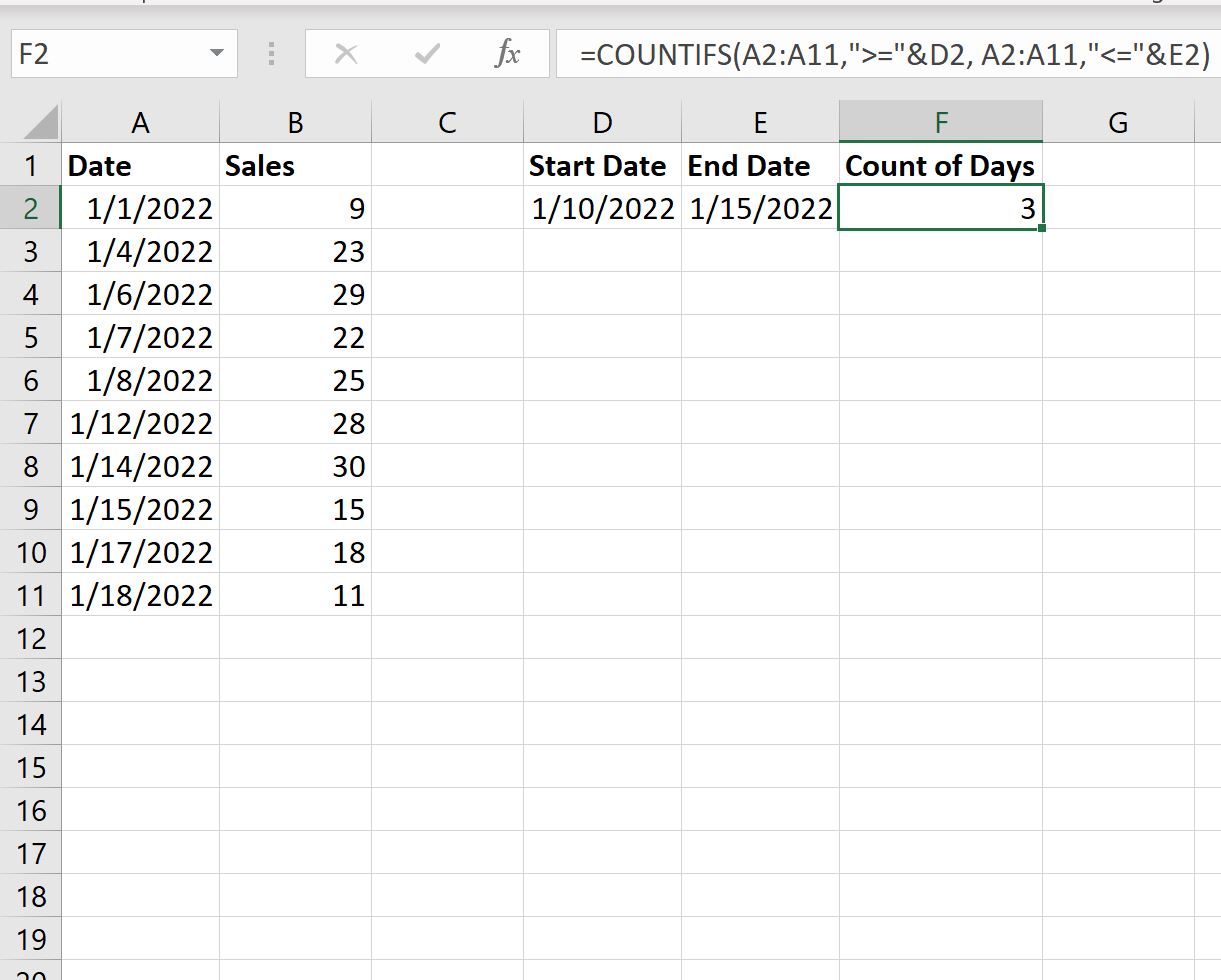
You can use the following syntax to count the number of cell values that fall in a date range in Excel:
=COUNTIFS(A2:A11,">="&D2, A2:A11,"<="&E2)
This formula counts the number of cells in the range A2:A11 where the date is between the dates in cells D2 and E2.
The following example shows how to use this syntax in practice.
Example: Use COUNTIFS with Date Range in Excel
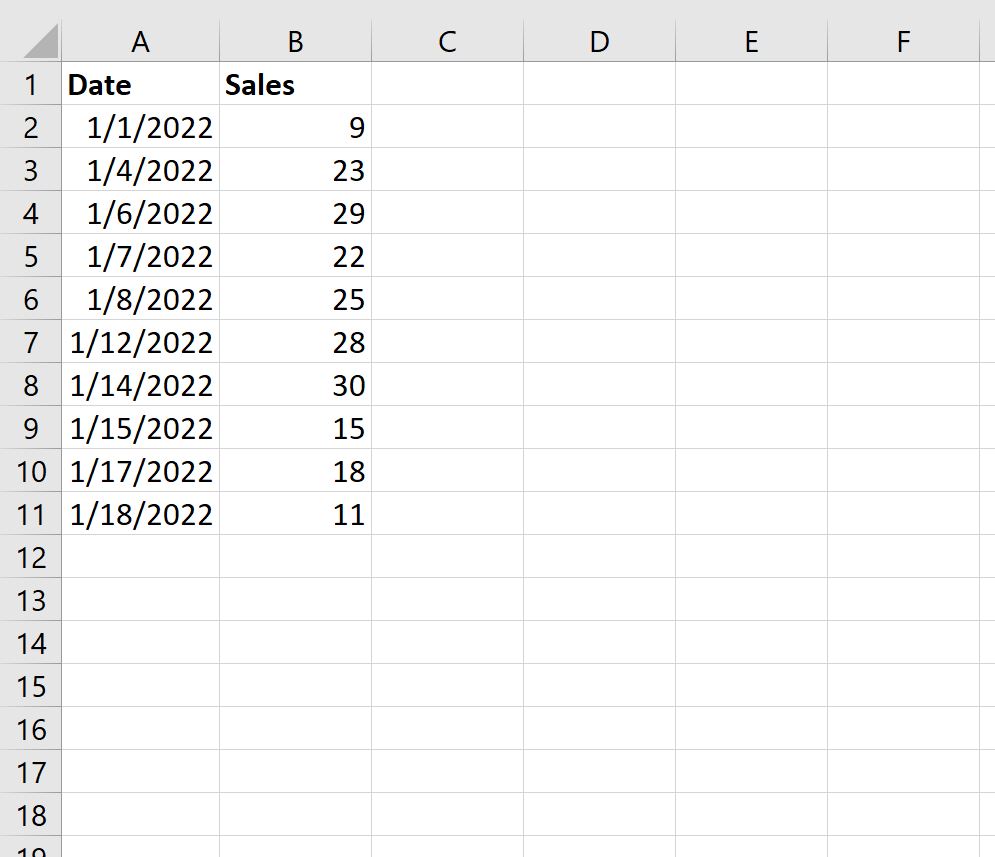
Suppose we have the following dataset in Excel that shows the number of sales made by some company on various days:

We can define a start and end date in cells D2 and E2 respectively, then use the following formula to count how many dates fall within the start and end date:
=COUNTIFS(A2:A11,">="&D2, A2:A11,"<="&E2)
The following screenshot shows how to use this formula in practice:

We can see that 3 days fall between 1/10/2022 and 1/15/2022.
We can manually verify that the following three dates in column A fall in this range:
- 1/12/2022
- 1/14/2022
- 1/15/2022
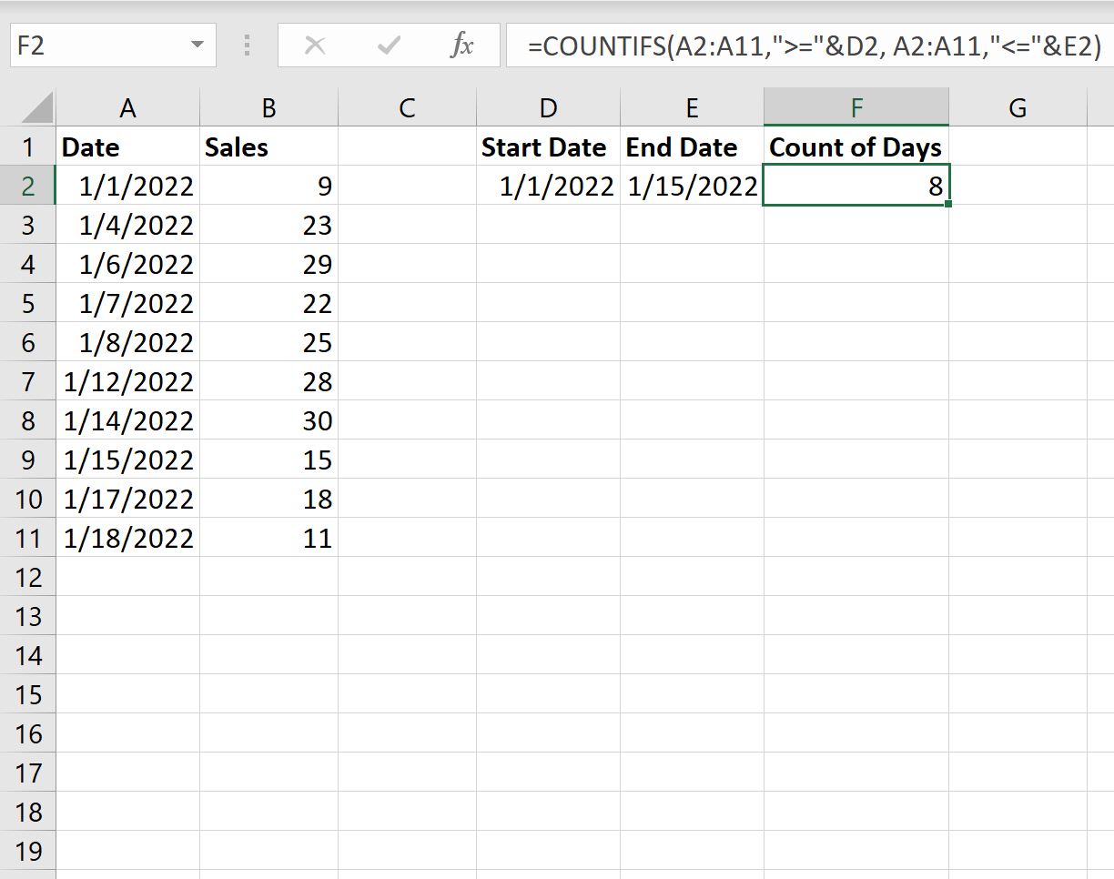
If we change either the start or end date, the formula will automatically update to count the cells within the new date range.
For example, suppose we change the start date to 1/1/2022:

We can see that 8 days fall between 1/1/2022 and 1/15/2022.
Additional Resources
The following tutorials provide additional information on how to work with dates in Excel:
How to Calculate Average If Between Two Dates in Excel
How to Calculate a Cumulative Sum by Date in Excel
How to Calculate the Difference Between Two Dates in Excel
17 авг. 2022 г.
читать 2 мин
Вы можете использовать следующий синтаксис для подсчета количества значений ячеек, попадающих в диапазон дат в Excel:
= COUNTIFS ( A2:A11 , ">=" & D2 , A2:A11 , "<=" & E2 )
Эта формула подсчитывает количество ячеек в диапазоне A2:A11 , где дата находится между датами в ячейках D2 и E2 .
В следующем примере показано, как использовать этот синтаксис на практике.
Пример: использование СЧЁТЕСЛИМН с диапазоном дат в Excel
Предположим, у нас есть следующий набор данных в Excel, который показывает количество продаж, совершенных какой-либо компанией в разные дни:
Мы можем определить дату начала и окончания в ячейках D2 и E2 соответственно, а затем использовать следующую формулу, чтобы подсчитать, сколько дат приходится на дату начала и окончания:
= COUNTIFS ( A2:A11 , ">=" & D2 , A2:A11 , "<=" & E2 )
На следующем снимке экрана показано, как использовать эту формулу на практике:
Мы видим, что между 10.01.2022 и 15.01.2022 приходится 3 дня.
Мы можем вручную проверить, что следующие три даты в столбце A попадают в этот диапазон:
- 12.01.2022
- 14.01.2022
- 15.01.2022
Если мы изменим дату начала или окончания, формула автоматически обновится, чтобы подсчитать ячейки в новом диапазоне дат.
Например, предположим, что мы изменили дату начала на 01.01.2022:
Мы видим, что между 01.01.2022 и 15.01.2022 приходится 8 дней.
Дополнительные ресурсы
В следующих учебниках представлена дополнительная информация о том, как работать с датами в Excel:
Как рассчитать среднее значение между двумя датами в Excel
Как рассчитать кумулятивную сумму по дате в Excel
Как рассчитать разницу между двумя датами в Excel
The COUNTIF function counts cells in a range that meet a given condition, referred to as criteria. COUNTIF is a common, widely used function in Excel, and can be used to count cells that contain dates, numbers, and text. Note that COUNTIF can only apply a single condition. To count cells with multiple criteria, see the COUNTIFS function.
Syntax
The generic syntax for COUNTIF looks like this:
=COUNTIF(range,criteria)The COUNTIF function takes two arguments, range and criteria. Range is the range of cells to apply a condition to. Criteria is the condition to apply, along with any logical operators that are needed.
Applying criteria
The COUNTIF function supports logical operators (>,<,<>,<=,>=) and wildcards (*,?) for partial matching. The tricky part about using the COUNTIF function is the syntax used to apply criteria. COUNTIFS is in a group of eight functions that split logical criteria into two parts, range and criteria. Because of this design, each condition requires a separate range and criteria argument, and operators in the criteria must be enclosed in double quotes («»). The table below shows examples of the syntax needed for common criteria:
| Target | Criteria |
|---|---|
| Cells greater than 75 | «>75» |
| Cells equal to 100 | 100 or «100» |
| Cells less than or equal to 100 | «<=100» |
| Cells equal to «Red» | «red» |
| Cells not equal to «Red» | «<>red» |
| Cells that are blank «» | «» |
| Cells that are not blank | «<>» |
| Cells that begin with «X» | «x*» |
| Cells less than A1 | «<«&A1 |
| Cells less than today | «<«&TODAY() |
Notice the last two examples involve concatenation with the ampersand (&) character. Any time you are using a value from another cell, or using the result of a formula in criteria with a logical operator like «<«, you will need to concatenate. This is because Excel needs to evaluate cell references and formulas first to get a value, before that value can be joined to an operator.
Basic example
In the worksheet shown above, the following formulas are used in cells G5, G6, and G7:
=COUNTIF(D5:D12,">100") // count sales over 100
=COUNTIF(B5:B12,"jim") // count name = "jim"
=COUNTIF(C5:C12,"ca") // count state = "ca"
Notice COUNTIF is not case-sensitive, «CA» and «ca» are treated the same.
Double quotes («») in criteria
In general, text values need to be enclosed in double quotes («»), and numbers do not. However, when a logical operator is included with a number, the number and operator must be enclosed in quotes, as seen in the second example below:
=COUNTIF(A1:A10,100) // count cells equal to 100
=COUNTIF(A1:A10,">32") // count cells greater than 32
=COUNTIF(A1:A10,"jim") // count cells equal to "jim"
Value from another cell
A value from another cell can be included in criteria using concatenation. In the example below, COUNTIF will return the count of values in A1:A10 that are less than the value in cell B1. Notice the less than operator (which is text) is enclosed in quotes.
=COUNTIF(A1:A10,"<"&B1) // count cells less than B1
Not equal to
To construct «not equal to» criteria, use the «<>» operator surrounded by double quotes («»). For example, the formula below will count cells not equal to «red» in the range A1:A10:
=COUNTIF(A1:A10,"<>red") // not "red"
Blank cells
COUNTIF can count cells that are blank or not blank. The formulas below count blank and not blank cells in the range A1:A10:
=COUNTIF(A1:A10,"<>") // not blank
=COUNTIF(A1:A10,"") // blank
Note: be aware that COUNTIF treats formulas that return an empty string («») as not blank. See this example for some workarounds to this problem.
Dates
The easiest way to use COUNTIF with dates is to refer to a valid date in another cell with a cell reference. For example, to count cells in A1:A10 that contain a date greater than the date in B1, you can use a formula like this:
=COUNTIF(A1:A10, ">"&B1) // count dates greater than A1
Notice we must concatenate an operator to the date in B1. To use more advanced date criteria (i.e. all dates in a given month, or all dates between two dates) you’ll want to switch to the COUNTIFS function, which can handle multiple criteria.
The safest way to hardcode a date into COUNTIF is to use the DATE function. This ensures Excel will understand the date. To count cells in A1:A10 that contain a date less than April 1, 2020, you can use a formula like this
=COUNTIF(A1:A10,"<"&DATE(2020,4,1)) // dates less than 1-Apr-2020
Wildcards
The wildcard characters question mark (?), asterisk(*), or tilde (~) can be used in criteria. A question mark (?) matches any one character and an asterisk (*) matches zero or more characters of any kind. For example, to count cells in A1:A5 that contain the text «apple» anywhere, you can use a formula like this:
=COUNTIF(A1:A5,"*apple*") // cells that contain "apple"
To count cells in A1:A5 that contain any 3 text characters, you can use:
=COUNTIF(A1:A5,"???") // cells that contain any 3 characters
The tilde (~) is an escape character to match literal wildcards. For example, to count a literal question mark (?), asterisk(*), or tilde (~), add a tilde in front of the wildcard (i.e. ~?, ~*, ~~).
OR logic
The COUNTIF function is designed to apply just one condition. However, to count cells that contain «this OR that», you can use an array constant and the SUM function like this:
=SUM(COUNTIF(range,{"red","blue"})) // red or blue
The formula above will count cells in range that contain «red» or «blue». Essentially, COUNTIF returns two counts in an array (one for «red» and one for «blue») and the SUM function returns the sum. For more information, see this example.
Limitations
The COUNTIF function has some limitations you should be aware of:
- COUNTIF only supports a single condition. If you need to count cells using multiple criteria, use the COUNTIFS function.
- COUNTIF requires an actual range for the range argument; you can’t provide an array. This means you can’t alter values in range before applying criteria.
- COUNTIF is not case-sensitive. Use the EXACT function for case-sensitive counts.
- COUNTIFS has other quirks explained in this article.
The most common way to work around the limitations above is to use the SUMPRODUCT function. In the current version of Excel, another option is to use the newer BYROW and BYCOL functions.
Notes
- Text strings in criteria must be enclosed in double quotes («»), i.e. «apple», «>32», «app*»
- Cell references in criteria are not enclosed in quotes, i.e. «<«&A1
- The wildcard characters ? and * can be used in criteria. A question mark matches any one character and an asterisk matches any sequence of characters (zero or more).
- To match a literal question mark(?) or asterisk (*), use a tilde (~) like (~?, ~*).
- COUNTIF requires a range, you can’t substitute an array.
- COUNTIF returns incorrect results when used to match strings longer than 255 characters.
- COUNTIF will return a #VALUE error when referencing another workbook that is closed.
Excel tables with their functions come in handy to count cells with data, horizontally and vertically. COUNTIF is the common function for counting cells with one and several conditions. So let’s look into this further to understand all the details and distinctions.
Meaning of COUNTIF Excel
COUNTIF in Excel is a statistical function that counts cells with those data that users indicate. It takes into account one condition.
- You can find items recorded even for months under a specific name.
- You may count the number of cells that hold a common letter or sign.
- You can use the Excel COUNTIF not blank to learn the empty cells quantity.
- You specify numerosity more or less than a mentioned value.
The COUNTIF formula in Excel consists of range (which goes first) and criteria (indicates the corresponding position).
=COUNTIF (range, criterion) rangeis the mandatory argument, which includes cells needed to find.criterionincludes expression, word, figures, letter, or other conditions that you need to discover.
How to use COUNTIF in Excel?
The function works with only one condition. Nevertheless, a person may single out many different data in turn. The computation is carried out with numbers, letters, words, phrases and dates. You can only write a cell reference or an entire condition. Sometimes, wildcards and symbols assist to determine more accurate values.
How COUNTIF works in Excel?
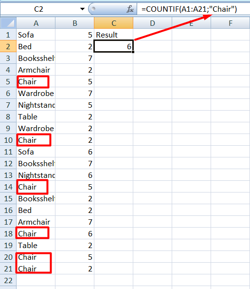
The function calculates the number of cells with indicated context, i.e., with the data that the user needs to count. For instance, you have a chart with diversified furniture bought over time. You may count what furniture (sofa, bed, wardrobe, chair, table, etc.) people buy. The COUNTIF will compute the cells in which the mentioned furniture is located. You write down the formula according to the condition you ought to detect. For example, let’s count the number of cells containing the word ‘chair‘:
=COUNTIF(A1:A21,"Chair")
Does COUNTIF function in Excel work for several criteria?
The COUNTIF doesn’t support frequentative conditions. Thus, you won’t find the number of chairs or nightstands purchased only in January or only on February 3. You have to use COUNTIFS for such cases.
However, you may write COUNTIF + COUNTIF. Such a COUNTIF Excel multiple criteria function makes the outcome more complete. Let’s determine the number of purchased chairs and sofas. Write the following:
=COUNTIF(A2:A21,"Chair")+COUNTIF(A2:A21,"Sofa").

Samples of advanced COUNTIFS function in Excel
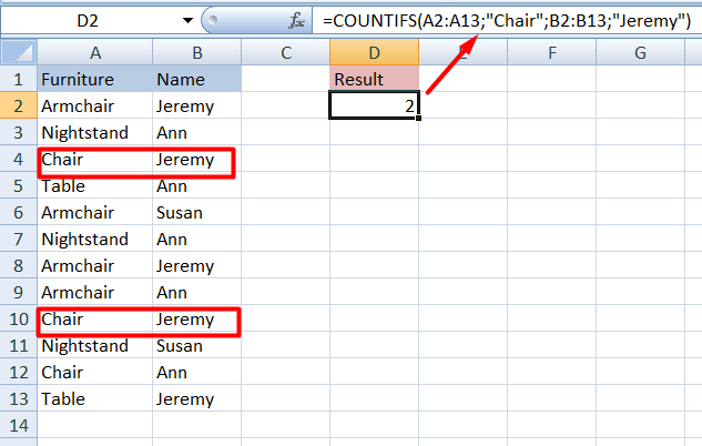
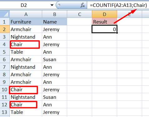
COUNTIF and COUNTIFS are various functions. They differ in the computation of cells with one criterion or more criteria. The first identifies cells under one condition, and the second takes into account several specific criteria. Let’s count the number of chairs bought by Jeremy. We need to use COUNTIFS for such appointments. Write it as follows:
=COUNTIFS(A2:A13,"Chair",B2:B13,"Jeremy")
Using COUNTIF in Excel when data is on other sources
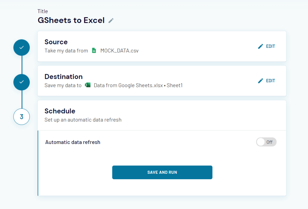
People usually store data on certain apps, such as Harvest, Google Drive, Jira, Pipedrive, etc. When you need to calculate this data in Excel, you can import it from the app. The Coupler.io tool is designed exactly for this. It will help transfer all the necessary information to BigQuery, Google Sheets, or Excel from other sources. In addition, you can automate updates to make your work easier in the future.

Sign up to Coupler.io and complete two steps to set up your Excel integration: source and destination. If you want to schedule automatic data refresh, you’ll need to configure one more step – schedule. Here is what the integration may look like:
Practical skills based on a COUNTIF Excel example
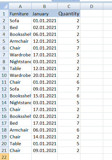
Examine a few samples of use in more detail. Take, for instance, the furniture in the store. Imagine the owner created an Excel table regarding sales. They write down the furniture in one column there. The other column contains the dates when the goods were sold. Finally, the third column contains the quantity of each product sold. So, let’s define some samples with several formulas, including dates, words and figures.
Excel COUNTIF: Cells are equal or not equal
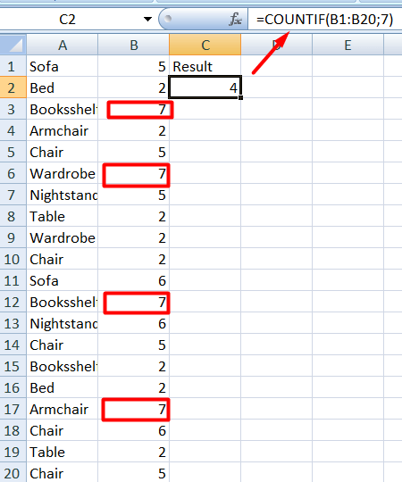
Imagine that people have bought every subject several times. Let’s take, for example, 7 times. In our formula, we specify the range where to look and the figure 7.
=COUNTIF(B1:B20,7)
Let’s still find the purchased furniture that isn’t equal to 5.
=COUNTIF(B1:B20,"<>5")

Excel COUNTIF: cells contain words
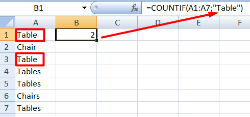
Let’s try to work with words using the same formula. Imagine that we need to know how many tables people bought. Let’s write the following formula.
=COUNTIF(A2:A21,"Table")

As a result, people bought 2 tables. You can replace the word with a cell reference
=COUNTIF(A2:A21,E2)

COUNTIF use in Excel – meaning of wildcards
We can use COUNTIF not only with words but also with special wildcards (* and ?) to generalize the condition.
?= One character.*= Sequence.
Also, you can write ~ to find symbols * or ?.
Let’s look at a simple formula
=COUNTIF(A1:A7,"Table")
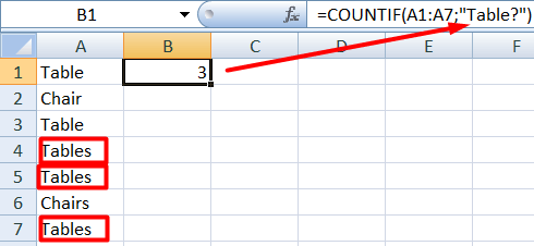
The question mark symbol ? adds one additional character. In our dataset, there are the words ‘Table‘ and ‘Tables‘ with the last letter ‘s‘. So, Table? in the formula will look for the latter option:
=COUNTIF(A1:A7,"Table?")
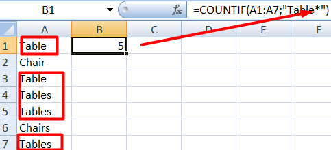
The asterisk symbol * adds a sequence of characters or even spaces. For instance, the following formula counts all words that start with Tab including ‘Table’ and ‘Tables’:
=COUNTIF(A1:A7,"Tab*")
Excel COUNTIF: сells are more than or less than
Let’s find out some values using operators: >, <, <>, =. We write it next to the criterion in quotation marks. Thanks to them, we can find cells with numbers that are more or less, equal, or not equal to some value. For example, let’s count the amount of furniture that people bought more than 3 times:
=COUNTIF(B1:B20,">3")

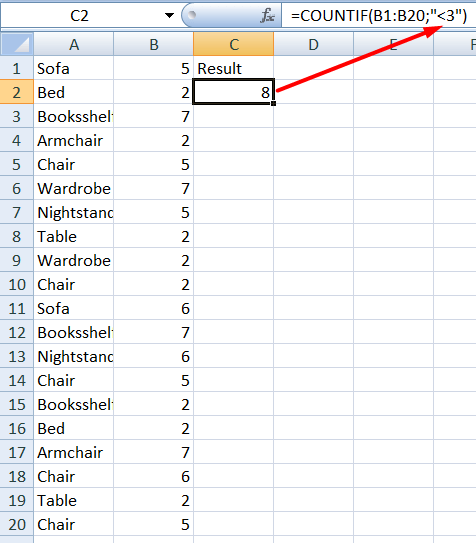
Change the logical operator to count the amount of furniture that people bought less than 3 times:
=COUNTIF(B1:B20,"<3")
Excel COUNTIF: count cells including date
Another feature is working with dates. So, let’s imagine that the biggest purchases fall on the date of January 1. We need to know the cells’ numerosity with this data.
=COUNTIF(B2:B21,"01/01/2021")

What common problems should you avoid?
Often, people face issues using the function. We seem to be doing everything right, but the Excel function COUNTIF shows the error. Look at a few situations why it occurs. For instance, you wrote the formula
=COUNTIF(A2:A13,Chair)
The function has shown zero results although this is not correct. So taking a closer look, the word ‘Chair‘ should be in quotation marks.
=COUNTIF(A2:A13,"Chair")
In another example of incorrect syntax, the formula returned #NAME?. In this case, there is a space between the range (A1:A7) and the criterion, which also has not quotation marks (Table).

The correct formula should look like this
=COUNTIF(A1:A7,"Table")
Best practices in using the COUNTIF function
It is easy to make mistakes both out of ignorance and inattention. However, by applying the following tips you can avoid the common mistakes.
- Write the wildcards (
?and*) to generalize the condition. - The condition can only have less than 255 characters. You will see an error exceeding this limit. To exceed the limit, you can use CONCATENATE or ampersand (&).
- The function returns the same value if the words are written in uppercase or lowercase letters. It doesn’t take into account case strings. You should rename the word if it has a different meaning.
- Pay attention to the spelling of words and letters. The function does not differentiate case strings and doesn’t work with misspellings.
Adherence to all principles and rules and writing correct syntax will facilitate calculations without problems. The main point is to write the formula and condition correctly.
-

Technical Content Writer on Coupler.io who loves working with data, writing about it, and even producing videos about it. I’ve worked at startups and product companies, writing content for technical audiences of all sorts. You’ll often see me cycling🚴🏼♂️, backpacking around the world🌎, and playing heavy board games.

Back to Blog
Focus on your business
goals while we take care of your data!
Try Coupler.io