
COUNTIF function
Use COUNTIF, one of the statistical functions, to count the number of cells that meet a criterion; for example, to count the number of times a particular city appears in a customer list.
In its simplest form, COUNTIF says:
-
=COUNTIF(Where do you want to look?, What do you want to look for?)
For example:
-
=COUNTIF(A2:A5,»London»)
-
=COUNTIF(A2:A5,A4)

COUNTIF(range, criteria)
|
Argument name |
Description |
|---|---|
|
range (required) |
The group of cells you want to count. Range can contain numbers, arrays, a named range, or references that contain numbers. Blank and text values are ignored. Learn how to select ranges in a worksheet. |
|
criteria (required) |
A number, expression, cell reference, or text string that determines which cells will be counted. For example, you can use a number like 32, a comparison like «>32», a cell like B4, or a word like «apples». COUNTIF uses only a single criteria. Use COUNTIFS if you want to use multiple criteria. |
Examples
To use these examples in Excel, copy the data in the table below, and paste it in cell A1 of a new worksheet.
|
Data |
Data |
|---|---|
|
apples |
32 |
|
oranges |
54 |
|
peaches |
75 |
|
apples |
86 |
|
Formula |
Description |
|
=COUNTIF(A2:A5,»apples») |
Counts the number of cells with apples in cells A2 through A5. The result is 2. |
|
=COUNTIF(A2:A5,A4) |
Counts the number of cells with peaches (the value in A4) in cells A2 through A5. The result is 1. |
|
=COUNTIF(A2:A5,A2)+COUNTIF(A2:A5,A3) |
Counts the number of apples (the value in A2), and oranges (the value in A3) in cells A2 through A5. The result is 3. This formula uses COUNTIF twice to specify multiple criteria, one criteria per expression. You could also use the COUNTIFS function. |
|
=COUNTIF(B2:B5,»>55″) |
Counts the number of cells with a value greater than 55 in cells B2 through B5. The result is 2. |
|
=COUNTIF(B2:B5,»<>»&B4) |
Counts the number of cells with a value not equal to 75 in cells B2 through B5. The ampersand (&) merges the comparison operator for not equal to (<>) and the value in B4 to read =COUNTIF(B2:B5,»<>75″). The result is 3. |
|
=COUNTIF(B2:B5,»>=32″)-COUNTIF(B2:B5,»<=85″) |
Counts the number of cells with a value greater than (>) or equal to (=) 32 and less than (<) or equal to (=) 85 in cells B2 through B5. The result is 1. |
|
=COUNTIF(A2:A5,»*») |
Counts the number of cells containing any text in cells A2 through A5. The asterisk (*) is used as the wildcard character to match any character. The result is 4. |
|
=COUNTIF(A2:A5,»?????es») |
Counts the number of cells that have exactly 7 characters, and end with the letters «es» in cells A2 through A5. The question mark (?) is used as the wildcard character to match individual characters. The result is 2. |
Common Problems
|
Problem |
What went wrong |
|---|---|
|
Wrong value returned for long strings. |
The COUNTIF function returns incorrect results when you use it to match strings longer than 255 characters. To match strings longer than 255 characters, use the CONCATENATE function or the concatenate operator &. For example, =COUNTIF(A2:A5,»long string»&»another long string»). |
|
No value returned when you expect a value. |
Be sure to enclose the criteria argument in quotes. |
|
A COUNTIF formula receives a #VALUE! error when referring to another worksheet. |
This error occurs when the formula that contains the function refers to cells or a range in a closed workbook and the cells are calculated. For this feature to work, the other workbook must be open. |
Best practices
|
Do this |
Why |
|---|---|
|
Be aware that COUNTIF ignores upper and lower case in text strings. |
|
|
Use wildcard characters. |
Wildcard characters —the question mark (?) and asterisk (*)—can be used in criteria. A question mark matches any single character. An asterisk matches any sequence of characters. If you want to find an actual question mark or asterisk, type a tilde (~) in front of the character. For example, =COUNTIF(A2:A5,»apple?») will count all instances of «apple» with a last letter that could vary. |
|
Make sure your data doesn’t contain erroneous characters. |
When counting text values, make sure the data doesn’t contain leading spaces, trailing spaces, inconsistent use of straight and curly quotation marks, or nonprinting characters. In these cases, COUNTIF might return an unexpected value. Try using the CLEAN function or the TRIM function. |
|
For convenience, use named ranges |
COUNTIF supports named ranges in a formula (such as =COUNTIF(fruit,»>=32″)-COUNTIF(fruit,»>85″). The named range can be in the current worksheet, another worksheet in the same workbook, or from a different workbook. To reference from another workbook, that second workbook also must be open. |
Note: The COUNTIF function will not count cells based on cell background or font color. However, Excel supports User-Defined Functions (UDFs) using the Microsoft Visual Basic for Applications (VBA) operations on cells based on background or font color. Here is an example of how you can Count the number of cells with specific cell color by using VBA.
Need more help?
You can always ask an expert in the Excel Tech Community or get support in the Answers community.

See also
COUNTIFS function
IF function
COUNTA function
Overview of formulas in Excel
IFS function
SUMIF function
Need more help?
EXPLANATION
This tutorial shows and explains how to count cells that do not contain a specific value using by using Excel formulas or VBA.
This tutorial provides two Excel methods that can be applied to count cells that do not contain a specific value in a selected range by using an Excel COUNTIF function combined with the not equal to sign (<>). The first method sources the value that from a cell, whilst the second method has the value (Exceldome) directly entered into the formula.
This tutorial provides two VBA methods that can be applied to count cells that do not contain a specific value in a selected range. The first method sources the value that from a cell, whilst the second method has the value (Exceldome) directly entered into the VBA code.
By including asterisk (*) in front and behind the value that we are searching for it will ensure that if there is other content in a cell, including the specific value, the formula will not count this cell.
FORMULA (value manually entered)
=COUNTIF(range,»<>»&»*value*»)
FORMULA (value sourced from cell reference)
=COUNTIF(range,»<>»&»*»&value&»*»)
ARGUMENTS
range: The range of cells you want to count from.
value: The value that is used to determine which of the cells should not be counted, from a specified range, if the cells contain this value.
In this article, we will learn about how to Count cells that do not contain value using COUNTIF function with wildcards in Excel.
In simple words, Consider a scenario in which we are required to count the data based on specific criteria in an array. counting cells that do not contain a specific value using wildcards to catch cell value with countif function in excel explained here with an example.
The COUNTIF function returns the count of cells that do not a specific value.
Syntax:
Range : array
Value : text in quotes and numbers without quotes.
<> : operator (not equal to)
Wildcard characters for catching strings and perform functions on it.
There are three wildcard characters in Excel
- Question mark ( ? ) : This wildcard is used to search for any single character.
- Asterisk ( * ): This wildcard is used to find any number of characters preceding or following any character.
- Tilde ( ~ ): This wildcard is an escape character, used preceding the question mark ( ? ) or asterisk mark( * ).
Let’s understand this function using it in an example.

There are different shades of colours in the array. We need to find the colours which do not have red.
Use the formula:
A2:A13 : array
<>*red* : condition where cells that don’t contain red in the cell value.

The red region marked are the 6 cells which do not contain red colour.
Now we will get the colours which do not have Blue
Use the formula:

There are 9 cells which do not have Blue.
Now we will get the colours which do not have Purple
Use the formula:
=COUNTIF(A2:A13,»<>*Purple*»)

As you can see the formula returns the count of cells which do not have a specific value.
Hope you understood how to use Indirect function and referring cell in Excel. Explore more articles on Excel function here. Please feel free to state your query or feedback for the above article.
Related Article:
How to Count Cells That Contain This Or That in Excel
How to Count Occurrences of a Word in an Excel Range in Excel
Get the COUNTIFS with Dynamic Criteria Range in Excel
How to Count total matches in two ranges in Excel
How to Count Unique Values In Excel
How To Count Unique Text in Excel
Popular Articles :
50 Excel Shortcut to Increase Your Productivity : Get faster at your task. These 50 shortcuts will make you work even faster on Excel.
How to use the VLOOKUP Function in Excel : This is one of the most used and popular functions of excel that is used to lookup value from different ranges and sheets.
How to use the COUNTIF function in Excel : Count values with conditions using this amazing function. You don’t need to filter your data to count specific values. Countif function is essential to prepare your dashboard.
How to use the SUMIF Function in Excel : This is another dashboard essential function. This helps you sum up values on specific conditions.
Explanation
In this example, the goal is to count the number of cells in column D that are not equal to a given color. The simplest way to do this is with the COUNTIF function, as explained below.
Not equal to
In Excel, the operator for not equal to is «<>». For example:
=A1<>10 // A1 is not equal to 10
=A1<>"apple" // A1 is not equal to "apple"
COUNTIF function
The COUNTIF function counts the number of cells in a range that meet supplied criteria:
=COUNTIF(range,criteria)
To use the not equal to operator (<>) in COUNTIF, it must be enclosed in double quotes like this:
=COUNTIF(range,"<>10") // not equal to 10
=COUNTIF(range,"<>apple") // not equal to "apple"
This is a requirement of COUNTIF, which is in a group of eight functions that share this syntax. In example shown, we want to count cells not equal to «red» in D5:D16, so we use «<>red» for criteria. The formula in G5 is:
=COUNTIF(D5:D16,"<>red") // returns 9
In cell G6, we count all cells not equal to blue with a similar formula:
=COUNTIF(D5:D16,"<>blue") // returns 7
Note: COUNTIF is not case-sensitive. The word «red» can appear in any combination of uppercase / lowercase letters.
Not equal to another cell
To use a value in another cell as part of the criteria, use the ampersand (&) operator to concatenate like this:
=COUNTIF(range,"<>"&A1)
For example, if A1 contains 100 the criteria will be «<>100» after concatenation, and COUNTIF will count cells not equal to 100:
=COUNTIF(range,"<>100")
COUNTIFS function
The COUNTIFs function is designed to handle multiple criteria, but can be used just like the COUNTIF function in this example:
=COUNTIFS(D5:D16,"<>red") // returns 9
=COUNTIFS(D5:D16,"<>blue") // returns 7
Video: How to use the COUNTIFS function
COUNTIF Not Blank Function
The COUNTIF not blank function counts non-blank cells within a range. The universal formula is “COUNTIF(range,”<>”&””)” or “COUNTIF(range,”<>”)”. This formula works with numbers, text, and date values. It also works with the logical operators like “<,” “>,” “=,” and so on.
Note: Alternatively, the COUNTA functionThe COUNTA function is an inbuilt statistical excel function that counts the number of non-blank cells (not empty) in a cell range or the cell reference. For example, cells A1 and A3 contain values but, cell A2 is empty. The formula “=COUNTA(A1,A2,A3)” returns 2.
read more can be used to count the non-blank cells.
Table of contents
- COUNTIF Not Blank Function
- How to Use COUNTIF Non-Blank Function?
- #1–Numerical Values
- #2–Text Values
- #3–Date Values
- The Characteristics of COUNTIF Not Blank Function
- Frequently Asked Questions
- Recommended Articles
- How to Use COUNTIF Non-Blank Function?
How to Use COUNTIF Non-Blank Function?
#1–Numerical Values
The steps to count non-empty cells with the help of the COUNTIF function are listed as follows:
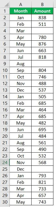
- In Excel, enter the following data containing both, the data cells and the empty cells.

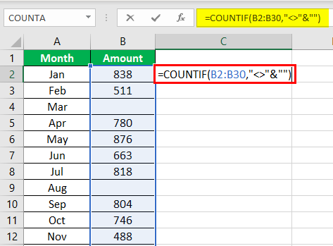
- Enter the following formula to count the data cells.
“=COUNTIF(range,”<>”&””)”
In the range argument, type B2:B30. Alternatively, select the range B2:B30 in the formula, as shown in the following image.

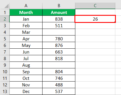
- Press the “Enter” key. The number of non-blank cells in the range B2:B30 appear in cell C2. The output is 26, as shown in the succeeding image.
This implies that there are 26 cells in the given range that contain a data value. This data can be a number, text, or any other value.

#2–Text Values
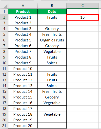
The steps to count non-empty cells within text values are listed as follows:
- Step 1: In Excel, enter the data as shown in the following image.
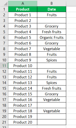
- Step 2: Select the range within which data needs to be checked for non-blank values. Enter the formula shown in the succeeding image.
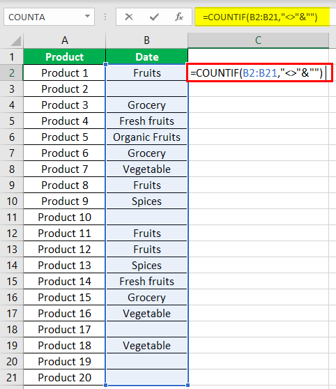
- Step 3: Press the “Enter” key. The number of non-blank cells in the range B2:B21 appear in cell C2. The output is 15, as shown in the succeeding image.
Hence, the COUNTIF not blank formula works with text values.
#3–Date Values
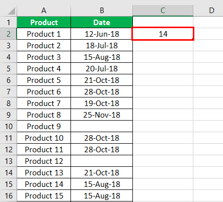
The steps to count non-empty cells, when the data consists of dates, are listed as follows:
- Step 1: In Excel, enter the data as shown in the following image. Select the range whose data needs to be checked for non-blank values. Enter the following formula.
“=COUNTIF(B2:B21,”<>”&””)”
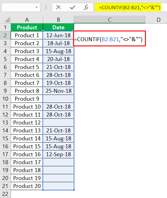
- Step 2: Press the “Enter” key. The number of non-blank cells in the range B2:B21 appear in cell C2. The output is 14, as shown in the succeeding image.
Hence, the COUNTIF not blank formula works with data that consists of date values.
The Characteristics of COUNTIF Not Blank Function
- It is case insensitive, implying that the output remains the same irrespective of whether the formula is entered in uppercase or lowercase.
- It works for data that consists of numbers, text, and date values.
- It works with greater than (>) and less than (<) operators.
- It is difficult to use the formula with long strings.
- The criteria (condition) must be specified within a pair of inverted commas to avoid errors.
Frequently Asked Questions
How is the COUNTIF formula used to count blanks?
The universal formula for counting blanks is stated as follows:
“COUNTIF(range,””)”
This formula works with all types of data values.
Note: Alternatively, the COUNTBLANK function can be used to count blank cells.
How does the COUNTIF function count the duplicate values?
The formula for counting the duplicate value is given as follows:
“COUNTIF(range,“duplicate value”)”
The “range” represents the range within which the duplicate values are to be counted. The “duplicate value” is the exact data value that is to be counted.
For example, to count the number of times the text “fruits” appears in the range A2:A10, we use “=COUNTIF(A2:A10,“fruits”).”
- The COUNTIF not blank function counts the non-blank cells within a given range.
- The generic formula of the COUNTIF not blank function is stated as–“COUNTIF (range,“<>”&””).”
- The criteria (condition) must be specified within a pair of inverted commas to avoid errors.
- The COUNTIF functionThe COUNTIF function in Excel counts the number of cells within a range based on pre-defined criteria. It is used to count cells that include dates, numbers, or text. For example, COUNTIF(A1:A10,”Trump”) will count the number of cells within the range A1:A10 that contain the text “Trump”
read more works for data that consists of numbers, text, and date values. - The COUNTIF formula gives the same output irrespective of whether the formula is entered in uppercase or lowercase.
Recommended Articles
This has been a guide to Excel COUNTIF not blank. Here we discuss how to use the COUNTIF function to count non-blank cells along with practical examples and a downloadable Excel template. You may learn more about Excel from the following articles –
- Not Equal in VBA
- COUNTIF with Multiple Criteria
- VLOOKUP Errors
- Use Not Equal to in Excel
- XML in Excel
Many a times we need to count cells based on a condition. However, sometimes the data may require us to count cells that are not equal to a specific value. Excel has a simple solution to count cells not equal to a certain value. We can use the The COUNTIF function can solve this problem very easily. In this article, we will learn how to count cells not equal to another value in Excel.
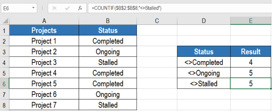 Figure 1. Example of How to Count Cells not Equal to in Excel
Generic Formula
=COUNTIF(range, <>value)
How this Formula Works
This formula is based on the COUNTIF function. We need to provide the range where we want to count the cells. The next argument is the value that we want to ignore during the count. COUNTIF will count all other values except this one.
First, COUNTIF counts the cells in the range that satisfies the condition we provide. We use the not equal to operator (<>) to count the cells in the range that does not equal to this value. This returns the count of cells other than this value.
Setting up Data
The following example uses a project information data set. Column A and B has the names and status of the projects. The statuses are “completed”, “ongoing” and “stalled”.
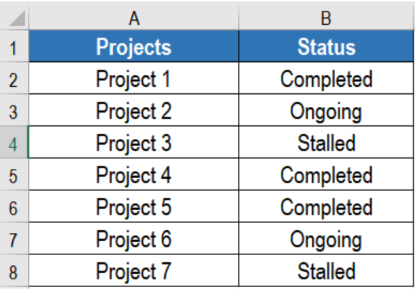 Figure 2. The Sample Data Set
To count the cells except the completed ones, we need to:
- Go to cell E4.
- Assign the formula
=COUNTIF($B$2:$B$8,”<>Completed”)to E4. - Press Enter.
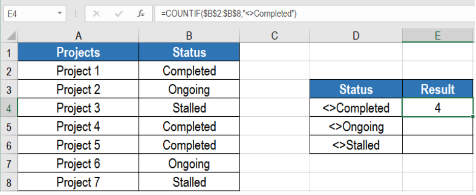 Figure 3. Applying the Formula
This will show the count of the projects except the completed ones. We can change this formula to find out the projects except the ongoing and stalled ones as well.
Notes
- COUNTIF is not case-sensitive. We can search for any combination of uppercase and lowercase letters.
- We can use a value from a cell as part of the criteria. To do this we need to use the ampersand character (&) to do this. To solve the previous example for project that are not stalled, we need to assign the formula
=COUNTIF(B2:B8,"<>"&B4)to E5.
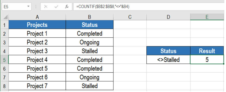 Figure 4. Count Cells not Equal to Using Cell References
This will show the number of projects except stalled in E5.
Most of the time, the problem you will need to solve will be more complex than a simple application of a formula or function. If you want to save hours of research and frustration, try our live Excelchat service! Our Excel Experts are available 24/7 to answer any Excel question you may have. We guarantee a connection within 30 seconds and a customized solution within 20 minutes.
You can use the following formulas to count the number of cells in Excel not equal to some value:
Method 1: Count Cells Not Equal to Value
=COUNTIF(A1:A100, "<>value")
This formula counts the number of cells in the range A1:A100 that are not equal to value.
Method 2: Count Cells Not Equal to Several Values
=COUNTIFS(A1:A100, "<>value1", A1:A100, "<>value2", A1:A100, "<>value3")
This formula counts the number of cells in the range A1:A100 that are not equal to value1 or value2 or value3.
The following examples show how to use each method in practice.
Example 1: Count Cells Not Equal to Value
Suppose we have the following data in Excel:

We can use the following formula to count the number of cells in the Team column that are not equal to “A”:
=COUNTIF(A2:A13, "<>A")
The following screenshot shows how to use this formula in practice:

This tells us that there are 10 cells in the Team column not equal to “A.”
Example 2: Count Cells Not Equal to Several Values
Once again suppose we have the following data in Excel:
We can use the following formula to count the number of cells in the Team column that are not equal to “A” or “B”:
=COUNTIFS(A2:A13, "<>A", A2:A13, "<>B")
The following screenshot shows how to use this formula in practice:

This tells us that there are 4 cells in the Team column not equal to “A” or “B.”
Additional Resources
The following tutorials explain how to perform other common tasks in Excel:
How to Count Filtered Rows in Excel
How to Use COUNTIF with OR in Excel
How to Use COUNTIF From Another Sheet in Excel
Have you ever been in a condition when you need to count cells in an Excel sheet?
Well, sometimes it is necessary to count cells as per your project’s requirements. And it happens when the COUNTIF not equal to a specific value. For this, Excel has specifically designed some functions that help you count values that are not equal to a specific value. The COUNTIF function is the one and only solution for this problem and here we will discuss it in detail.
First of all, let’s move on to the basic COUNTIF formula:
Basic Formula
=COUNTIF(range, <>Value)
How COUNTIF Formula Works?
The basis of this formula is the COUNTIF function, in which the range is needed that helps in counting the cells. In the formula, the next argument is the value that is no longer needed in the function. In the COUNTIF formula, all other values are important except this one.
The given condition is solved when the COUNTIF function counts the cells in the range. To count the cells available in the range, the not equal to the operator (<>) is used that never equals to this value.
How to Use COUNTIF to Count Cells Not Equal to X or Y
With the COUNTIF function, you can count cells that meet the criteria. Not equal operator (<>) is used to make a “not equal” logical statement, for instance “<>WATER.”
You need to add range criteria in the function to make an x or y logic. You can even add z logic with x and y. In the given example, you can see the COUNTIF counts cells in range Type(D3:D4) that is not equal to x(“Water”) or y(“FIRE”).

How to count cells not equal to a specific value
The COUNTIF function is needed to count cells that are not equal to a specific value. Well, this exactly counters the cells that are equal to. In the COUNTIF function, you need to count the number of cells given in the specific range that fulfills the specific criteria. The symbol “<>” is used that represents the condition not equal to for a value. Have a look at the following example.

In this example, you can see two conditions; first, the flights counting that didn’t arrive and the second one is the flights that are not rescheduled. This condition is done with the help of the COUNTIF function.
The COUNTIF not equal to a specific value – Formula Explained
=COUNTIF(D5:D10,”<>Arrived”)
At first, you can see the range, D5:D10 following an IF condition. Enter <>Arrived with double quotation marks like “<>Arrived” to find flights that have not arrived. From cells in D5:D10, this can return the count that is not equal to “Arrived”.
Likewise, in the second condition, you will see the flights counting that are not Rescheduled after modifying the criteria to “<>Rescheduled”.
Notice: Remember that the COUNTIF function is not case sensitive at all and the text values in COUNTIF criteria have to be in double quotes like this (“”).
Tips & Tricks: You can avoid errors by using a value in another cell as the criteria or a part of the criteria. Moreover, to concatenate you may use an ampersand (&) when a part of the criteria is in another cell.
Setting Up Data
In the following example, the project information data set is used. Two columns A and B appeared with the names and status as “completed”, “ongoing” and “Stalled”.

Other than the completed cells, to count the cells you have to:
- Go to cell E4
- Apply the formula =COUNTIF($B$2:$B$8,”<>Completed”) to E4.
- Press Enter

Doing this will show the projects counting rather than the completed ones. You can change this formula as per your requirements. Also, note that the COUNTIF function is not case-sensitive that’s why you can make any type of uppercase or lowercase letters combination.
As part of the criteria, you are free to use a value from a cell. For this, the ampersand & is used. In order to solve the previous example, you may need to apply the formula as =COUNTIF(B2:B8,”<>”&B4) to E5.

Doing this will display the projects excluding stalled in E5.
At times, the problem might be more complicated than simply applying the formula or a function. That’s why you always need to be careful every time you are assigning values to your data.
COUNTIF Not Equal to X
To apply one condition to the counting formula, you may use COUNTIF. The formula for COUNTIF can be written with data as COUNTIF not equal to cappuccino:
=COUNTIF(E23:E42, “<>cappuccino”)
As you already know that COUNTIFS use one compulsory condition and the rest are optional, that’s why you can write this formula as COUNTIFS not equal to cappuccino:
=COUNTIFS(E23:E42, “<>cappuccino”)
To Sum Up
COUNTIF is not equal to is a great thing to use in your Excel projects. Counting cells in a data set can be a tiring thing, however, with some simple functions you can make complex tasks easier. That’s why the COUNTIF function helps you in many conditions. And you need to be careful while using Excel functions.
Home / Excel Formulas / Count Blank (Empty) Cells using COUNTIF
If you want to count cells that are blank in Excel, you can use the COUNTBLANK function which is specifically designed to count cells that are empty (without any value in them). In the COUNTBLANK function, you just need to refer to the range from where you want to count the blank cells.
Use COUNTBLANK Function
In the following example, you have a few values in the range A1:A10, but a few of the cells are empty. And now, you need to count the cells those cells with no values in them.

You can use the following steps to write this formula:
- First, in cell B1, start typing the COUNTBLANK function (=COUNTBLANK).
- After that, Type the starting parentheses.
- Now, refer to the range A1:A10 in the function.
- In the end, type a closing parenthesis and hit enter.

=COUNTBLANK(A1:A10)Once you hit enter it returns the count of the cells that are blank in the specified range.

You can also use COUNTIF and create a condition to count blank cells. By using the same example, you can follow the below steps to write this formula:
- First, in cell B1, start typing the COUNTIF function (=COUNTIF), and enter starting parenthesis.
- Now, refer to the range A1:A10 from where you want to count the cells with no value.
- Next, in the criteria argument, type “=”. This equals operator tells Excel to count cells where you have no value because with the = operator you have not specified anything.
- After that, type the closing parentheses and hit enter.

And the moment, you hit enter it returns the count for blank cells.

You can also use a formula like the following with the “=”&”” criteria. When you use it, it also tells Excel to count only cells with no value in them.

Download Sample File
- Ready