Excel for Microsoft 365 Excel 2021 Excel 2019 Excel 2016 Excel 2013 Excel 2010 Excel 2007 More…Less
To count numbers or dates that meet a single condition (such as equal to, greater than, less than, greater than or equal to, or less than or equal to), use the COUNTIF function. To count numbers or dates that fall within a range (such as greater than 9000 and at the same time less than 22500), you can use the COUNTIFS function. Alternately, you can use SUMPRODUCT too.
Example
Note: You’ll need to adjust these cell formula references outlined here based on where and how you copy these examples into the Excel sheet.
|
1 |
A |
B |
|---|---|---|
|
2 |
Salesperson |
Invoice |
|
3 |
Buchanan |
15,000 |
|
4 |
Buchanan |
9,000 |
|
5 |
Suyama |
8,000 |
|
6 |
Suyma |
20,000 |
|
7 |
Buchanan |
5,000 |
|
8 |
Dodsworth |
22,500 |
|
9 |
Formula |
Description (Result) |
|
10 |
=COUNTIF(B2:B7,»>9000″) |
The COUNTIF function counts the number of cells in the range B2:B7 that contain numbers greater than 9000 (4) |
|
11 |
=COUNTIF(B2:B7,»<=9000″) |
The COUNTIF function counts the number of cells in the range B2:B7 that contain numbers less than 9000 (4) |
|
12 |
=COUNTIFS(B2:B7,»>=9000″,B2:B7,»<=22500″) |
The COUNTIFS function (available in Excel 2007 and later) counts the number of cells in the range B2:B7 greater than or equal to 9000 and are less than or equal to 22500 (4) |
|
13 |
=SUMPRODUCT((B2:B7>=9000)*(B2:B7<=22500)) |
The SUMPRODUCT function counts the number of cells in the range B2:B7 that contain numbers greater than or equal to 9000 and less than or equal to 22500 (4). You can use this function in Excel 2003 and earlier, where COUNTIFS is not available. |
|
14 |
Date |
|
|
15 |
3/11/2011 |
|
|
16 |
1/1/2010 |
|
|
17 |
12/31/2010 |
|
|
18 |
6/30/2010 |
|
|
19 |
Formula |
Description (Result) |
|
20 |
=COUNTIF(B14:B17,»>3/1/2010″) |
Counts the number of cells in the range B14:B17 with a data greater than 3/1/2010 (3) |
|
21 |
=COUNTIF(B14:B17,»12/31/2010″) |
Counts the number of cells in the range B14:B17 equal to 12/31/2010 (1). The equal sign is not needed in the criteria, so it is not included here (the formula will work with an equal sign if you do include it («=12/31/2010»). |
|
22 |
=COUNTIFS(B14:B17,»>=1/1/2010″,B14:B17,»<=12/31/2010″) |
Counts the number of cells in the range B14:B17 that are between (inclusive) 1/1/2010 and 12/31/2010 (3). |
|
23 |
=SUMPRODUCT((B14:B17>=DATEVALUE(«1/1/2010»))*(B14:B17<=DATEVALUE(«12/31/2010»))) |
Counts the number of cells in the range B14:B17 that are between (inclusive) 1/1/2010 and 12/31/2010 (3). This example serves as a substitute for the COUNTIFS function that was introduced in Excel 2007. The DATEVALUE function converts the dates to a numeric value, which the SUMPRODUCT function can then work with. |
Need more help?
EXPLANATION
This tutorial shows and explains how to count cells that do not contain a specific value using by using Excel formulas or VBA.
This tutorial provides two Excel methods that can be applied to count cells that do not contain a specific value in a selected range by using an Excel COUNTIF function combined with the not equal to sign (<>). The first method sources the value that from a cell, whilst the second method has the value (Exceldome) directly entered into the formula.
This tutorial provides two VBA methods that can be applied to count cells that do not contain a specific value in a selected range. The first method sources the value that from a cell, whilst the second method has the value (Exceldome) directly entered into the VBA code.
By including asterisk (*) in front and behind the value that we are searching for it will ensure that if there is other content in a cell, including the specific value, the formula will not count this cell.
FORMULA (value manually entered)
=COUNTIF(range,»<>»&»*value*»)
FORMULA (value sourced from cell reference)
=COUNTIF(range,»<>»&»*»&value&»*»)
ARGUMENTS
range: The range of cells you want to count from.
value: The value that is used to determine which of the cells should not be counted, from a specified range, if the cells contain this value.
The COUNTIF function counts cells in a range that meet a given condition, referred to as criteria. COUNTIF is a common, widely used function in Excel, and can be used to count cells that contain dates, numbers, and text. Note that COUNTIF can only apply a single condition. To count cells with multiple criteria, see the COUNTIFS function.
Syntax
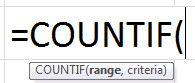
The generic syntax for COUNTIF looks like this:
=COUNTIF(range,criteria)The COUNTIF function takes two arguments, range and criteria. Range is the range of cells to apply a condition to. Criteria is the condition to apply, along with any logical operators that are needed.
Applying criteria
The COUNTIF function supports logical operators (>,<,<>,<=,>=) and wildcards (*,?) for partial matching. The tricky part about using the COUNTIF function is the syntax used to apply criteria. COUNTIFS is in a group of eight functions that split logical criteria into two parts, range and criteria. Because of this design, each condition requires a separate range and criteria argument, and operators in the criteria must be enclosed in double quotes («»). The table below shows examples of the syntax needed for common criteria:
| Target | Criteria |
|---|---|
| Cells greater than 75 | «>75» |
| Cells equal to 100 | 100 or «100» |
| Cells less than or equal to 100 | «<=100» |
| Cells equal to «Red» | «red» |
| Cells not equal to «Red» | «<>red» |
| Cells that are blank «» | «» |
| Cells that are not blank | «<>» |
| Cells that begin with «X» | «x*» |
| Cells less than A1 | «<«&A1 |
| Cells less than today | «<«&TODAY() |
Notice the last two examples involve concatenation with the ampersand (&) character. Any time you are using a value from another cell, or using the result of a formula in criteria with a logical operator like «<«, you will need to concatenate. This is because Excel needs to evaluate cell references and formulas first to get a value, before that value can be joined to an operator.
Basic example
In the worksheet shown above, the following formulas are used in cells G5, G6, and G7:
=COUNTIF(D5:D12,">100") // count sales over 100
=COUNTIF(B5:B12,"jim") // count name = "jim"
=COUNTIF(C5:C12,"ca") // count state = "ca"
Notice COUNTIF is not case-sensitive, «CA» and «ca» are treated the same.
Double quotes («») in criteria
In general, text values need to be enclosed in double quotes («»), and numbers do not. However, when a logical operator is included with a number, the number and operator must be enclosed in quotes, as seen in the second example below:
=COUNTIF(A1:A10,100) // count cells equal to 100
=COUNTIF(A1:A10,">32") // count cells greater than 32
=COUNTIF(A1:A10,"jim") // count cells equal to "jim"
Value from another cell
A value from another cell can be included in criteria using concatenation. In the example below, COUNTIF will return the count of values in A1:A10 that are less than the value in cell B1. Notice the less than operator (which is text) is enclosed in quotes.
=COUNTIF(A1:A10,"<"&B1) // count cells less than B1
Not equal to
To construct «not equal to» criteria, use the «<>» operator surrounded by double quotes («»). For example, the formula below will count cells not equal to «red» in the range A1:A10:
=COUNTIF(A1:A10,"<>red") // not "red"
Blank cells
COUNTIF can count cells that are blank or not blank. The formulas below count blank and not blank cells in the range A1:A10:
=COUNTIF(A1:A10,"<>") // not blank
=COUNTIF(A1:A10,"") // blank
Note: be aware that COUNTIF treats formulas that return an empty string («») as not blank. See this example for some workarounds to this problem.
Dates
The easiest way to use COUNTIF with dates is to refer to a valid date in another cell with a cell reference. For example, to count cells in A1:A10 that contain a date greater than the date in B1, you can use a formula like this:
=COUNTIF(A1:A10, ">"&B1) // count dates greater than A1
Notice we must concatenate an operator to the date in B1. To use more advanced date criteria (i.e. all dates in a given month, or all dates between two dates) you’ll want to switch to the COUNTIFS function, which can handle multiple criteria.
The safest way to hardcode a date into COUNTIF is to use the DATE function. This ensures Excel will understand the date. To count cells in A1:A10 that contain a date less than April 1, 2020, you can use a formula like this
=COUNTIF(A1:A10,"<"&DATE(2020,4,1)) // dates less than 1-Apr-2020
Wildcards
The wildcard characters question mark (?), asterisk(*), or tilde (~) can be used in criteria. A question mark (?) matches any one character and an asterisk (*) matches zero or more characters of any kind. For example, to count cells in A1:A5 that contain the text «apple» anywhere, you can use a formula like this:
=COUNTIF(A1:A5,"*apple*") // cells that contain "apple"
To count cells in A1:A5 that contain any 3 text characters, you can use:
=COUNTIF(A1:A5,"???") // cells that contain any 3 characters
The tilde (~) is an escape character to match literal wildcards. For example, to count a literal question mark (?), asterisk(*), or tilde (~), add a tilde in front of the wildcard (i.e. ~?, ~*, ~~).
OR logic
The COUNTIF function is designed to apply just one condition. However, to count cells that contain «this OR that», you can use an array constant and the SUM function like this:
=SUM(COUNTIF(range,{"red","blue"})) // red or blue
The formula above will count cells in range that contain «red» or «blue». Essentially, COUNTIF returns two counts in an array (one for «red» and one for «blue») and the SUM function returns the sum. For more information, see this example.
Limitations
The COUNTIF function has some limitations you should be aware of:
- COUNTIF only supports a single condition. If you need to count cells using multiple criteria, use the COUNTIFS function.
- COUNTIF requires an actual range for the range argument; you can’t provide an array. This means you can’t alter values in range before applying criteria.
- COUNTIF is not case-sensitive. Use the EXACT function for case-sensitive counts.
- COUNTIFS has other quirks explained in this article.
The most common way to work around the limitations above is to use the SUMPRODUCT function. In the current version of Excel, another option is to use the newer BYROW and BYCOL functions.
Notes
- Text strings in criteria must be enclosed in double quotes («»), i.e. «apple», «>32», «app*»
- Cell references in criteria are not enclosed in quotes, i.e. «<«&A1
- The wildcard characters ? and * can be used in criteria. A question mark matches any one character and an asterisk matches any sequence of characters (zero or more).
- To match a literal question mark(?) or asterisk (*), use a tilde (~) like (~?, ~*).
- COUNTIF requires a range, you can’t substitute an array.
- COUNTIF returns incorrect results when used to match strings longer than 255 characters.
- COUNTIF will return a #VALUE error when referencing another workbook that is closed.
Return to Excel Formulas List
Download Example Workbook
Download the example workbook
This tutorial demonstrates how to use the COUNTIF function to determine if a value exists in a range.
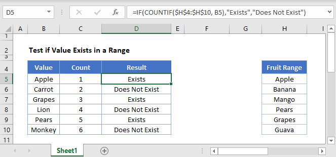
COUNTIF Value Exists in a Range
To test if a value exists in a range, we can use the COUNTIF Function:
=COUNTIF(Range, Criteria)>0The COUNTIF function counts the number of times a condition is met. We can use the COUNTIF function to count the number of times a value appears in a range. If COUNTIF returns greater than 0, that means that value exists.
=COUNTIF($E$3:$E$9,B3)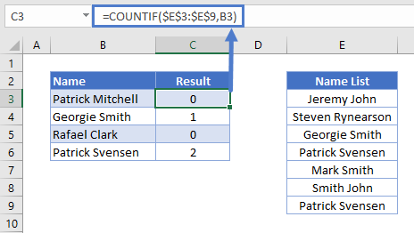
By attaching “>0” to the end of the COUNTIF Function, we test if the function returns >0. If so, the formula returns TRUE (the value exists).
=COUNTIF($E$3:$E$9,B3)>0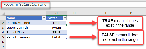
You can see above that the formula results in a TRUE statement for the name “Patrick Mitchell. On the other hand, the name “Georgia Smith” and “Patrick Svensen” does not exist in the range $B$2:$B$31.
You can wrap this formula around an IF Function to output a specific result. For example, if we want to add a “Does not exist” text for names that are not in the list, we can use the following formula:
=IF(COUNTIF($B$2:$B$31, Name)>0, “Exists”, “Does Not Exist”)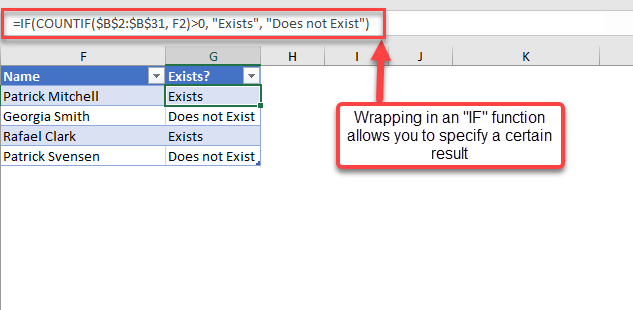
COUNTIF Value Exists in a Range Google Sheets
We use the same formula structure in Google Sheets:
=IF(COUNTIF(Range, Criteria)>0, “Exists”, “Does Not Exist”)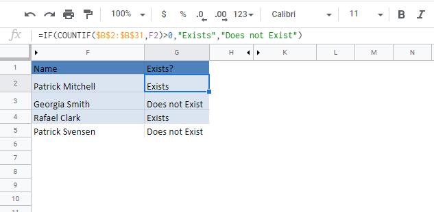
COUNTIF Not Blank Function
The COUNTIF not blank function counts non-blank cells within a range. The universal formula is “COUNTIF(range,”<>”&””)” or “COUNTIF(range,”<>”)”. This formula works with numbers, text, and date values. It also works with the logical operators like “<,” “>,” “=,” and so on.
Note: Alternatively, the COUNTA functionThe COUNTA function is an inbuilt statistical excel function that counts the number of non-blank cells (not empty) in a cell range or the cell reference. For example, cells A1 and A3 contain values but, cell A2 is empty. The formula “=COUNTA(A1,A2,A3)” returns 2.
read more can be used to count the non-blank cells.
Table of contents
- COUNTIF Not Blank Function
- How to Use COUNTIF Non-Blank Function?
- #1–Numerical Values
- #2–Text Values
- #3–Date Values
- The Characteristics of COUNTIF Not Blank Function
- Frequently Asked Questions
- Recommended Articles
- How to Use COUNTIF Non-Blank Function?
How to Use COUNTIF Non-Blank Function?
#1–Numerical Values
The steps to count non-empty cells with the help of the COUNTIF function are listed as follows:
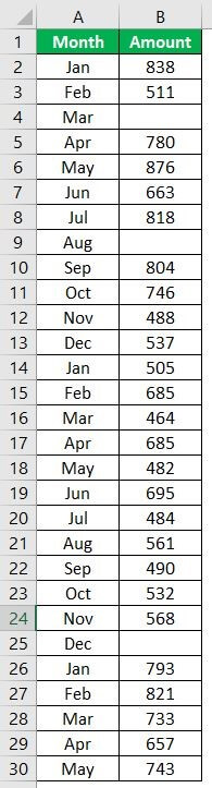
- In Excel, enter the following data containing both, the data cells and the empty cells.

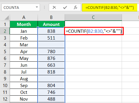
- Enter the following formula to count the data cells.
“=COUNTIF(range,”<>”&””)”
In the range argument, type B2:B30. Alternatively, select the range B2:B30 in the formula, as shown in the following image.

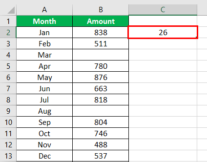
- Press the “Enter” key. The number of non-blank cells in the range B2:B30 appear in cell C2. The output is 26, as shown in the succeeding image.
This implies that there are 26 cells in the given range that contain a data value. This data can be a number, text, or any other value.

#2–Text Values
The steps to count non-empty cells within text values are listed as follows:
- Step 1: In Excel, enter the data as shown in the following image.
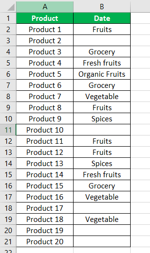
- Step 2: Select the range within which data needs to be checked for non-blank values. Enter the formula shown in the succeeding image.
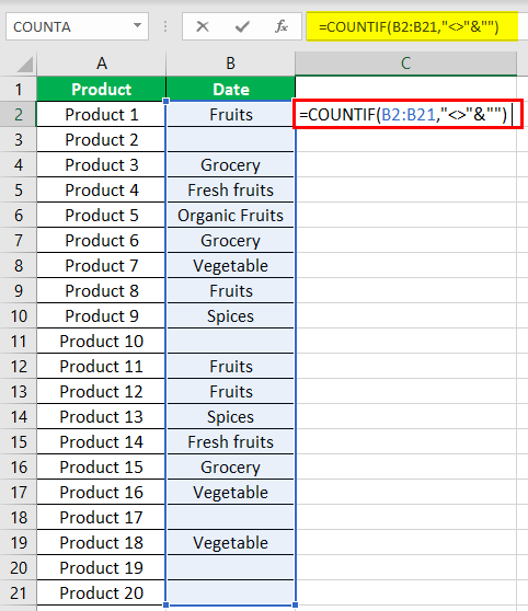
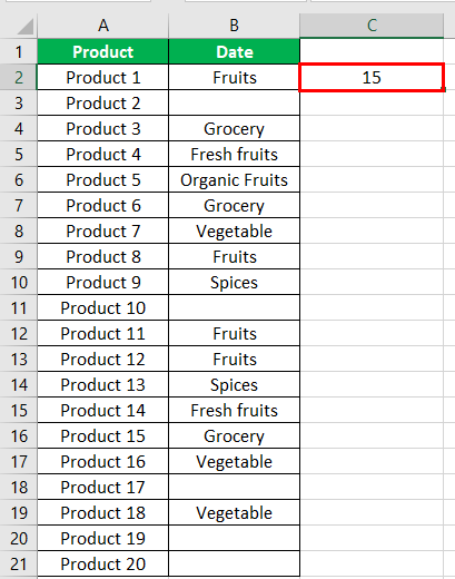
- Step 3: Press the “Enter” key. The number of non-blank cells in the range B2:B21 appear in cell C2. The output is 15, as shown in the succeeding image.
Hence, the COUNTIF not blank formula works with text values.
#3–Date Values
The steps to count non-empty cells, when the data consists of dates, are listed as follows:
- Step 1: In Excel, enter the data as shown in the following image. Select the range whose data needs to be checked for non-blank values. Enter the following formula.
“=COUNTIF(B2:B21,”<>”&””)”
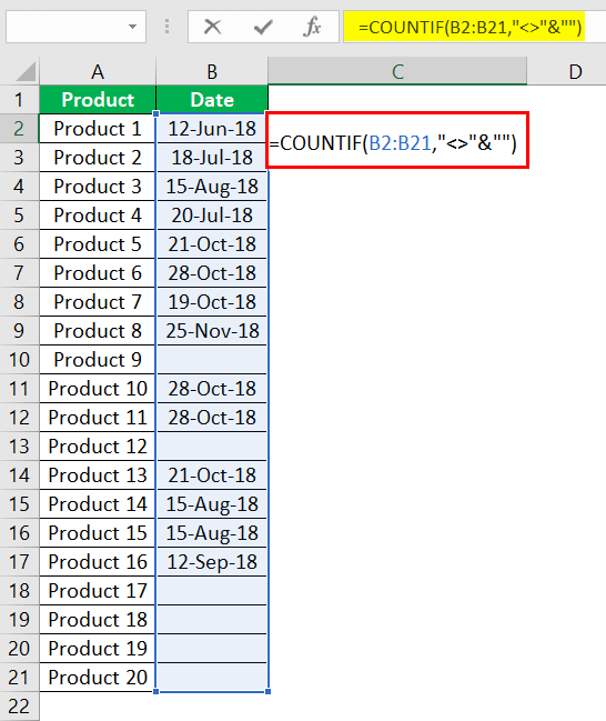
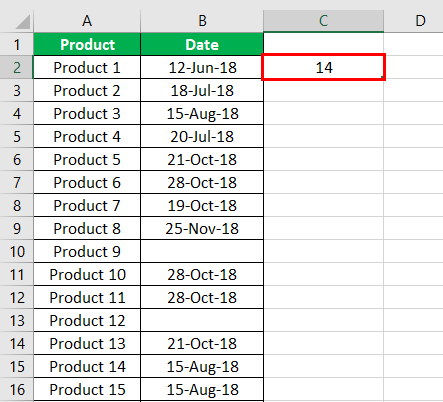
- Step 2: Press the “Enter” key. The number of non-blank cells in the range B2:B21 appear in cell C2. The output is 14, as shown in the succeeding image.
Hence, the COUNTIF not blank formula works with data that consists of date values.
The Characteristics of COUNTIF Not Blank Function
- It is case insensitive, implying that the output remains the same irrespective of whether the formula is entered in uppercase or lowercase.
- It works for data that consists of numbers, text, and date values.
- It works with greater than (>) and less than (<) operators.
- It is difficult to use the formula with long strings.
- The criteria (condition) must be specified within a pair of inverted commas to avoid errors.
Frequently Asked Questions
How is the COUNTIF formula used to count blanks?
The universal formula for counting blanks is stated as follows:
“COUNTIF(range,””)”
This formula works with all types of data values.
Note: Alternatively, the COUNTBLANK function can be used to count blank cells.
How does the COUNTIF function count the duplicate values?
The formula for counting the duplicate value is given as follows:
“COUNTIF(range,“duplicate value”)”
The “range” represents the range within which the duplicate values are to be counted. The “duplicate value” is the exact data value that is to be counted.
For example, to count the number of times the text “fruits” appears in the range A2:A10, we use “=COUNTIF(A2:A10,“fruits”).”
- The COUNTIF not blank function counts the non-blank cells within a given range.
- The generic formula of the COUNTIF not blank function is stated as–“COUNTIF (range,“<>”&””).”
- The criteria (condition) must be specified within a pair of inverted commas to avoid errors.
- The COUNTIF functionThe COUNTIF function in Excel counts the number of cells within a range based on pre-defined criteria. It is used to count cells that include dates, numbers, or text. For example, COUNTIF(A1:A10,”Trump”) will count the number of cells within the range A1:A10 that contain the text “Trump”
read more works for data that consists of numbers, text, and date values. - The COUNTIF formula gives the same output irrespective of whether the formula is entered in uppercase or lowercase.
Recommended Articles
This has been a guide to Excel COUNTIF not blank. Here we discuss how to use the COUNTIF function to count non-blank cells along with practical examples and a downloadable Excel template. You may learn more about Excel from the following articles –
- Not Equal in VBA
- COUNTIF with Multiple Criteria
- VLOOKUP Errors
- Use Not Equal to in Excel
- XML in Excel
Want to learn more about how to count cells do not contain using Excel spreadsheet?? This post will give you an overview of how to use COUNTIF formula functions to get the number of cells that do not contain using Excel.
Syntax(Generic Formula)
=COUNTIF(range,”<>*txt*”)
How COUNTIF & COUNTIFS work
Excel has many syntax for a user who needs to specify on counting the total amount of cells with single or multiple criteria. For example, if you want to count cells based on more than one or more criteria, you can use the COUNTIF or COUNTIFS functions in Excel.
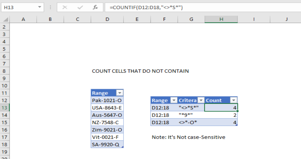 Figure 1: Example of count cells that do not contain
To count cells that do not contain, you can use the COUNTIF function. In the example shown, the formula in H13 is
=COUNTIF(D10:D18”<>”S”)
Difference Between COUNTIF & COUNTIFS
The difference between COUNTIF and COUNTIFS function is about the total number of condition that applies. While COUNTIF is designed to count the cells with a single condition, COUNTIFS function will let you have several criteria indifferent or in the same range as you wish.
=COUNTIFS(range”<>*?*”,rang”?*”)
By this tutorial, you have learned how to count the number of cells which don’t contain a specific text string.
Still need some help with Excel formatting or have other questions about Excel? Connect with a live Excel expert here for some 1 on 1 help. Your first session is always free.
So, there are times when you would like to know that a value is in a list or not. We have done this using VLOOKUP. But we can do the same thing using COUNTIF function too. So in this article, we will learn how to check if a values is in a list or not using various ways.
Check If Value In Range Using COUNTIF Function
So as we know, using COUNTIF function in excel we can know how many times a specific value occurs in a range. So if we count for a specific value in a range and its greater than zero, it would mean that it is in the range. Isn’t it?
Generic Formula
=COUNTIF(range,value)>0
Range: The range in which you want to check if the value exist in range or not.
Value: The value that you want to check in the range.
Let’s see an example:
Excel Find Value is in Range Example
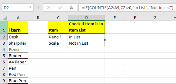
For this example, we have below sample data. We need a check-in the cell D2, if the given item in C2 exists in range A2:A9 or say item list. If it’s there then, print TRUE else FALSE.
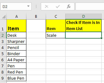
Write this formula in cell D2:
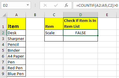
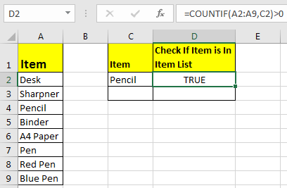
Since C2 contains “scale” and it’s not in the item list, it shows FALSE. Exactly as we wanted. Now if you replace “scale” with “Pencil” in the formula above, it’ll show TRUE.
Now, this TRUE and FALSE looks very back and white. How about customizing the output. I mean, how about we show, “found” or “not found” when value is in list and when it is not respectively.
Since this test gives us TRUE and FALSE, we can use it with IF function of excel.
Write this formula:
=IF(COUNTIF(A2:A9,C2)>0,»in List»,»Not in List»)
You will have this as your output.
What If you remove “>0” from this if formula?
=IF(COUNTIF(A2:A9,C2),»in List»,»Not in List»)
It will work fine. You will have same result as above. Why? Because IF function in excel treats any value greater than 0 as TRUE.
How to check if a value is in Range with Wild Card Operators
Sometimes you would want to know if there is any match of your item in the list or not. I mean when you don’t want an exact match but any match.
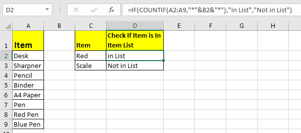
For example, if in the above-given list, you want to check if there is anything with “red”. To do so, write this formula.
=IF(COUNTIF(A2:A9,»*red*»),»in List»,»Not in List»)
This will return a TRUE since we have “red pen” in our list. If you replace red with pink it will return FALSE. Try it.
Now here I have hardcoded the value in list but if your value is in a cell, say in our favourite cell B2 then write this formula.
IF(COUNTIF(A2:A9,»*»&B2&»*»),»in List»,»Not in List»)
There’s one more way to do the same. We can use the MATCH function in excel to check if the column contains a value. Let’s see how.
Find if a Value is in a List Using MATCH Function
So as we all know that MATCH function in excel returns the index of a value if found, else returns #N/A error. So we can use the ISNUMBER to check if the function returns a number.
If it returns a number ISNUMBER will show TRUE, which means it’s found else FALSE, and you know what that means.
Write this formula in cell C2:
=ISNUMBER(MATCH(C2,A2:A9,0))
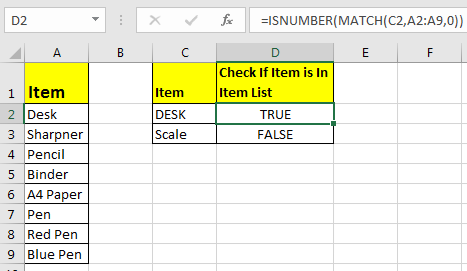
The MATCH function looks for an exact match of value in cell C2 in range A2:A9. Since DESK is on the list, it shows a TRUE value and FALSE for SCALE.
So yeah, these are the ways, using which you can find if a value is in the list or not and then take action on them as you like using IF function. I explained how to find value in a range in the best way possible. Let me know if you have any thoughts. The comments section is all yours.
Related Articles:
How to Check If Cell Contains Specific Text in Excel
How to Check A list of Texts In String in Excel
How to take the Average Difference between lists in Excel
How to Get Every Nth Value From A list in Excel
Popular Articles:
50 Excel Shortcuts to Increase Your Productivity
How to use the VLOOKUP Function in Excel
How to use the COUNTIF function in Excel
How to use the SUMIF Function in Excel
This post will guide you how to count the number of cells that are not equal to many things in a given range cells using a formula in Excel 2013/2016. You can easily to count cells not equal to a specific value through COUNTIF function. But if there is an easy way to count cells which are not equal to one of many values defined in a selected range of cells in Microsoft Excel. You can count cells that are not equal to many things with a combined formula based on the SUMPRODUCT function, the ISNA function and the MATCH function.
Table of Contents
- Count Cells not equal to one of many Things
- Related Functions
Actually, if you just have two or three things that you don’t want to count in your data list, and you can only use one COUNTIFS function like below:
=COUNTIFS(A2:A6,”<>excel”,A2:A6,”<>word”)
The above formula does not scale very well if you have a list of many things that you do not count, since you have to add more range and criteria pair to for each thing that you do not want to count in range. In this case, you can use the MATCH function to find cells in range A2:A6 that are not equal to values in range D1:D2 like this:
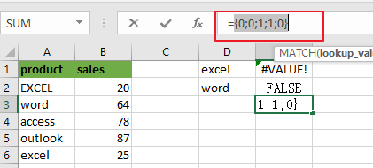
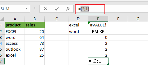
=MATCH(A2:A6,D1:D2,0)
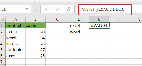
Pressing “Fn” + “F9” or “F9” short key to display the array results like this:
={1;2;#N/A;#N/A;1}
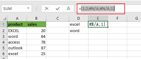
A2:A6 is the lookup value and D1:D2 is the lookup array. Since there are more than one lookup value in range D1:D2, so it returns more than one result in an array result like below:
MATCH function returns the position of lookup values in the lookup array, if lookup value is not in lookup array, it will return #N/A errors. Actually, the numbers of “#N/A” is the number of cells that are not equal to things in D1:D2.
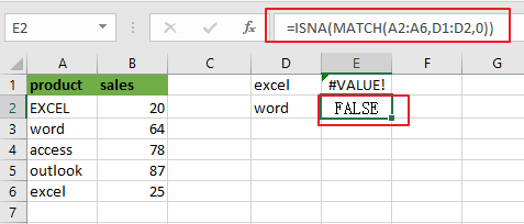
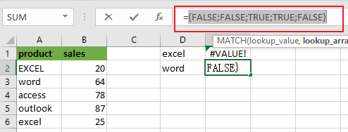
Then you can use the ISNA function to convert all values in the above array result to TRUE or FALSE, like below:
=ISNA(MATCH(A2:A6,D1:D2,0))
={FALSE;FALSE;TRUE;TRUE;FALSE}
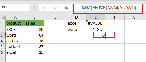
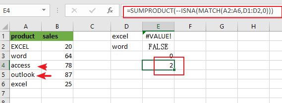
Next, you need to use a double negative operator to convert TRUE or FALSE value as 1 or 0 in the above array result. Like below:
=–ISNA(MATCH(A2:A6,D1:D2,0))
={0;0;1;1;0}
Last, passing the above resulting array to the SUMPRODUCT or SUM function looks like below:
=SUMPRODUCT(–ISNA(MATCH(A2:A6,D1:D2,0)))
Or
{=SUM(–ISNA(MATCH(A2:A6,D1:D2,0)))}
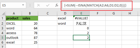
Note: if you are using SUM function in the above formula, you need to press “CTRL + SHIFT + ENTER” shortcuts to convert the formula as a array formula. And the SUMPRMDUCT function can handle the array result by itself.
You can also use another method to count cells which are not equal to many things with a combined formula that utilizes the COUNTA, SUMPRODUCT, and COUNTIF functions.
The general formula is like this:
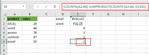
=COUNTA(range)-SUMPRODUCT(COUNTIF(range, things))
In this case, use the following formula:
=COUNTA(A2:A6)-SUMPRODUCT(COUNTIF(A2:A6, D1:D2))
Let’s see how this formula works:
The COUNTA function will count all of the cells in the range A2:A6. And the total number of cell in range A2:A6 is 5.
The COUNTIF function will check the range A2:A6 that contain the values in range D1:D2. Then it returns an array result like this:
=COUNTIF(A2:A6, D1:D2)
={2;1}
The SUMPRODUCT function adds up all numbers in the above resulting array, then the returned number is subtracted from the count of all the values in range A2:A6.
The solution logic is that calculating the count of cells that having specific values and then subtract it from the count of all non-empty cells in range A2:A6.
- Excel SUMPRODUCT function
The Excel SUMPRODUCT function multiplies corresponding components in the given one or more arrays or ranges, and returns the sum of those products. The syntax of the SUMPRODUCT function is as below:= SUMPRODUCT (array1,[array2],…)… - Excel COUNTIF function
The Excel COUNTIF function will count the number of cells in a range that meet a given criteria. This function can be used to count the different kinds of cells with number, date, text values, blank, non-blanks, or containing specific characters. etc. = COUNTIF (range, criteria) … - Excel MATCH function
The Excel MATCH function search a value in an array and returns the position of that item.The MATCH function is a build-in function in Microsoft Excel and it is categorized as a Lookup and Reference Function.The syntax of the MATCH function is as below:= MATCH (lookup_value, lookup_array, [match_type])…. - Excel COUNTIFS function
The Excel COUNTIFS function returns the count of cells in a range that meet one or more criteria. The syntax of the COUNTIFS function is as below:= COUNTIFS(criteria_range1, criteria1, [criteria_range2, criteria2]…)… - Excel SUM function
The Excel SUM function will adds all numbers in a range of cells and returns the sum of these values. You can add individual values, cell references or ranges in excel.The syntax of the SUM function is as below:= SUM(number1,[number2],…) - Excel ISNA function
The Excel ISNA function used to check if a cell contains the #N/A error, if so, returns TRUE; otherwise, the ISNA function returns FALSE.The syntax of the ISNA function is as below:=ISNA(value)…. - Excel COUNTA function
The Excel COUNTA function counts the number of cells that are not empty in a range. The syntax of the COUNTA function is as below:= COUNTA(value1, [value2],…)…
Blank cells
COUNTIF can count cells that are blank or not blank. The formulas below count blank and not blank cells in the range A1:A10:
Note: be aware that COUNTIF treats formulas that return an empty string («») as not blank. See this example for some workarounds to this problem.
Dates
The easiest way to use COUNTIF with dates is to refer to a valid date in another cell with a cell reference. For example, to count cells in A1:A10 that contain a date greater than the date in B1, you can use a formula like this:
Notice we must concatenate an operator to the date in B1. To use more advanced date criteria (i.e. all dates in a given month, or all dates between two dates) you’ll want to switch to the COUNTIFS function, which can handle multiple criteria.
The safest way to hardcode a date into COUNTIF is to use the DATE function. This ensures Excel will understand the date. To count cells in A1:A10 that contain a date less than April 1, 2020, you can use a formula like this
Wildcards
The wildcard characters question mark (?), asterisk(*), or tilde (
) can be used in criteria. A question mark (?) matches any one character and an asterisk (*) matches zero or more characters of any kind. For example, to count cells in A1:A5 that contain the text «apple» anywhere, you can use a formula like this:
To count cells in A1:A5 that contain any 3 text characters, you can use:
) is an escape character to match literal wildcards. For example, to count a literal question mark (?), asterisk(*), or tilde (
), add a tilde in front of the wildcard (i.e.
OR logic
The COUNTIF function is designed to apply just one condition. However, to count cells that contain «this OR that», you can use an array constant and the SUM function like this:
The formula above will count cells in range that contain «red» or «blue». Essentially, COUNTIF returns two counts in an array (one for «red» and one for «blue») and the SUM function returns the sum. For more information, see this example.
Limitations
The COUNTIF function has some limitations you should be aware of:
- COUNTIF only supports a single condition. If you need to count cells using multiple criteria, use the COUNTIFS function.
- COUNTIF requires an actual range for the range argument; you can’t provide an array. This means you can’t alter values in range before applying criteria.
- COUNTIF is not case-sensitive. Use the EXACT function for case-sensitive counts.
- COUNTIFS has other quirks explained in this article.
The most common way to work around the limitations above is to use the SUMPRODUCT function. In the current version of Excel, another option is to use the newer BYROW and BYCOL functions.
Источник
COUNTIF Function in Excel


What is COUNTIF Function in Excel
The COUNTIF function in Excel counts the number of cells within a range based on pre-defined criteria. It is used to count cells that include dates, numbers, or text. For example, COUNTIF(A1:A10,”Trump”) will count the number of cells within the range A1:A10 that contain the text “Trump”
Syntax
The syntax of COUNTIF formula in Excel is stated as follows:
It accepts the following required arguments:
- Range: It represents the range of values on which the criteria will be applied.
- Criteria: It represents the condition that is applied to the range of values. The values that meet the criteria are returned as a result.
The output of the COUNTIF formula is a positive number which can be zero or non-zero.
Table of contents
How to Use COUNTIF Function in Excel?
Let us consider some uses to understand the working of the COUNTIF excel function.
#1 – Count Values with the Given Value
The following table shows a list containing numerical values in the cells A2:A7. Count the given range of cells for the values matching the number “33”.
The COUNTIF function is applied to the given range of cells, and the formula is stated as follows:
Here the condition applied to the formula is the number “33”.The formula checks the range of cells A2:A7 for the values matching number “33”. The range contains only one such number, which satisfies the condition. Hence the result returned by the COUNTIF function is “1”. The result is displayed in cell A8.

#2 – Count Numbers with a Value Less Than the Given Number
A list of data in the cells A12:A17 is provided in the succeeding table. Count the given range of cells for the values less than “50”.
The COUNTIF function is applied to the given range of cells, and the formula is stated as follows:
“=COUNTIF(A12:A17,“ 
#3 – Count Values with the Given Text Value
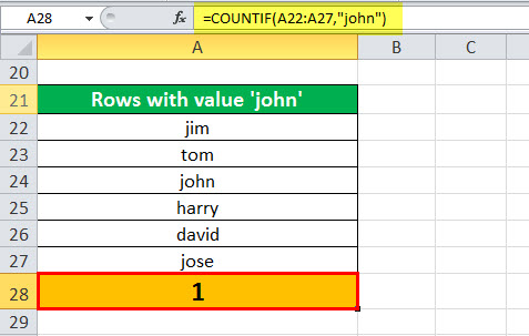
A list of data in the cells A22:A27 is provided in the below table. Count the range of cells for the text value “john”.
The COUNTIF function is applied to the given range of cells, and the formula is stated as follows:
Here the condition applied to the formula is the value “john.” The COUNTIF formula checks the range of cells matching the given condition. The given range has only one cell that satisfies the text value “john”. Hence, the result is “1” which is displayed in cell A28.
#4 – Count Negative Numbers
A list of data in the range of cells A32:A37 is provided in the below table. Count the range of cells for negative values (that is, less than zero).
The COUNTIF function is applied to the given range of cells, and the formula is stated as follows:
“=COUNTIF(A32:A37, “ 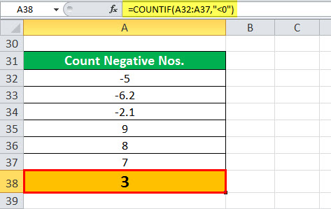
#5 – Count Zero Values
A list of data in the range of cells A42:A47 is provided in the below table. Count the range of cells for the value “0”.
The COUNTIF function is applied to the given range of cells, and the formula is stated as follows:
Here the condition applied to the formula is equal to “0”. Now the COUNTIF formula will identify and count the numbers with zero values. There are two zeros in the range. Hence, the result returned is “2” which is displayed in cell A48.

The Criteria of the COUNTIF Formula
It is enclosed within double quotes if non-numeric and without quotes if numeric.
It returns the result only if the values in the cell range satisfy the given criteria.
It can be supplied with wildcard characters like “*” and “?”. The question mark matches any one of the characters, and the asterisk matches any sequence of characters.
It uses the tilde operators followed by the wildcard characters such as “
Frequently Asked Questions (FAQs)
COUNTIF function allows counting of the range of cells that meets the specified criteria. It is used to count cells that contain dates, numbers, and text.
The formula is stated as follows:
“=COUNTIF(range,criteria)”
Where,
• “Range” is a required parameter that refers to the range on which the criteria will be applied.
• “Criteria” is another required parameter that represents the condition applied to the values of the range.
The syntax of COUNTIF function for the same range of cells (“range 1”) with multiple criteria (“criteria 1”, “criteria 2”) is as follows:
“=COUNTIF(range 1,criteria 1)+COUNTIF(range 1,criteria 2)”
In the case of counting multiple ranges of cells with multiple criteria, the COUNTIFS function can be used.
COUNTIFS function is used to evaluate cells across multiple ranges, based on single or multiple conditions. It is similar to the COUNTIF, but multiple criteria are used in the formula.
The formula of the COUNTIFS is stated as follows:
“=COUNTIFS(range 1, criteria1, range 2, criteria 2… )”
Where,
• “Range” refers to the given range of cells.
• “Criteria” refers to the conditions applied to the range.
Video
Recommended Articles
This has been a guide to the COUNTIF function in Excel. In this article, we have discussed how to use COUNTIF formula along with case studies and downloadable templates. You may also look at the below useful functions in Excel –
Источник
Excel VBA CountIf: How to Count Specific Values in a Range
The COUNTIF function allows you to count the number of cells that meet a specific condition. It’s one of Excel’s most useful functions for data calculations and analysis. This blog post will show you how to use COUNTIF Excel VBA and provide some examples. Read on for all the details!
Excel VBA: COUNTIF function
COUNTIF is a function that counts the number of cells based on the criteria you specify. It combines COUNT and IF, and allows you to put in one criterion when doing the count. You can use this function, for example, to quickly get the number of products in a particular category, to find how many students scored higher than 80, and so on.
You can simply use COUNTIF in a cell’s formula by entering =COUNTIF(range, criteria) . We have a helpful article that explains how to use Excel COUNTIF in a worksheet — so if you ever need a refresher, just give it a read!
In some cases, however, you may need to write VBA COUNTIF function as a part of automation tasks in Excel. Let’s say, every day, you need to automatically import data from multiple external sources, process the data, summarize it using COUNTIF and other statistical functions, and finally send a report in PDF or Powerpoint. Automating that process using VBA is a great way to improve productivity and save time!
Tip: As a shortcut for getting data from multiple different sources into Excel, use an integration tool like Coupler.io. With Coupler.io’s powerful integration with Excel, you can easily import data from Airtable, Jira, Xero, plus many more into Excel on the schedule you want! The process happens automatically without any coding on your part! So, this can be an additional great time saver for you.

VBA COUNTIF syntax and parameters
COUNTIF is an Excel worksheet function. To write this function in VBA, specify the function name prefixed by WorksheetFunction , as follows:

As you can see in the above image, COUNTIF returns Double and has two required arguments:
| Name | Data type | Description |
| Arg1 | Range | Range. The range of cells to count. |
| Arg2 | Variant | Criterion. The criterion that defines which cells will be counted. It can be a number, text, expression, or cell reference. For example: 85, “red”, “ You can use the wildcard characters (? and *) in COUNTIF for more flexible criteria. This can be helpful if you want to do partial matching. For example:
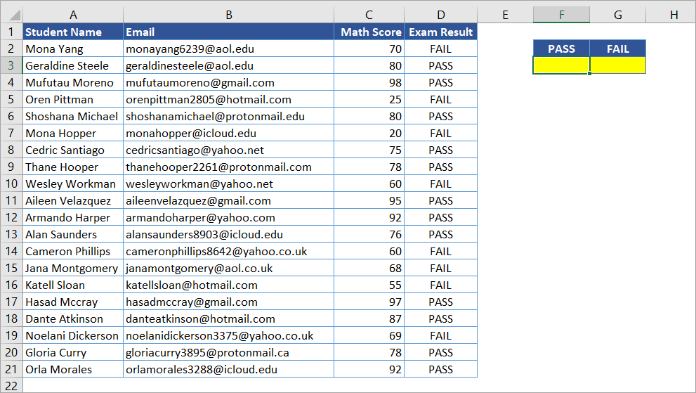
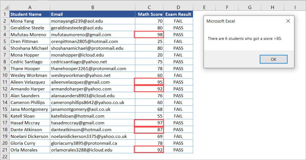
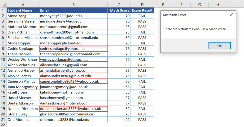
*” as the criteria. A tilde ( ) followed by a wildcard character matches the character. COUNTIF VBA Excel: Download an example fileYou can download the following Excel file to follow along with the examples in this article: The file contains a list of students and their scores on a Math exam. After adding VBA codes, save it as a macro-enabled workbook (.xlsm). How to use COUNTIF in VBA: A basic exampleWith the following student data, suppose you want to find how many students have passed vs. failed the math exam. The following steps show you how to create a Sub procedure (macro) in VBA to get the result using VBA Excel COUNTIF:
As you can see, the results of both Subs in F3 and G3 are values, not formulas. This makes the results not change if any of the values in range D2:D21 change. If you’d like to see formulas in the cells, you can write the code slightly differently, as shown in the below Subs: Here’s an example result in F3: COUNTIF function VBA: More examplesThere are many ways to use COUNTIF VBA Excel. We’ll take a look at examples with operators, wildcards, multiple criteria, and more. COUNTIF VBA example #1: Using operatorsOperators (such as >, >=, ) can be used in COUNTIF’s criteria. For example, you can use the “>” operator to only count cells that are higher than a certain value. The following COUNTIF VBA code counts the number of students who got a score higher than 85: The code above uses three variables with different data types. First is rng , which stores the range of cells to count. The second is criteria , which holds the criteria we want to specify. The last is result , which stores the output of the COUNTIF function. In this case, we are counting the cells in the range C2:C21 where its value is higher than 85. We use the “>” operator and combine it with the criteria using an ampersand symbol. The calculation result is stored in the result variable. Finally, the code outputs a message box showing the result: COUNTIF VBA example #2: Using wildcards for partial matchingThe following COUNTIF in VBA counts the students who use Yahoo emails: The function uses the “*” symbol at the beginning and end of the criteria to match all emails containing a Yahoo address. Notice that the criteria are not case-sensitive. Here’s the output: COUNTIF VBA example #3: Multiple OR criteriaYou can use multiple COUNTIFs (COUNTIF+COUNTIF+…) for multiple OR criteria in one column. For example, you could use COUNTIFs to count the number of cells that contain “red” OR “blue.” With our student dataset, you can use the following code to see how many students got scores higher than 95 OR lower than 25: The solution is simple and straightforward. You can just use multiple COUNTIFs if you have more than one OR criteria in a single column. Here’s the output of the above code: COUNTIF VBA example #4: Multiple AND criteriaSuppose you need to count the number of students who use Yahoo email AND have a math score higher than 90. COUNTIF does not work in this case. The COUNTIFS function might be the solution you’re looking for. You can also get the result manually using a loop, but we recommend you use COUNTIFS if possible. Code 1: Using COUNTIFS In the code below, we use the COUNTIFS function with 4 parameters: 2 range and 2 criteria parameters. Here’s the output: Code 2: Manually count in a loop The below code loops from Row 2 to 21 and checks all values in Column B and Column C. If there is a match, the result variable is incremented by 1. For Column B, the Like operator is used to find a partial match. Notice that it’s case-sensitive, so we apply LCase when making the comparison. There might be a time when you might want to do processing in a loop. For example, if you’re trying to count cells by checking if they’re bold or having certain colors, etc., which can’t be done using COUNTIFS alone. COUNTIF VBA example #5: Using COUNTIF to highlight duplicatesThere are times when you have large amounts of data with duplicates. Instead of using the Remove Duplicates command on the Data tab, you might want to just mark them for future reference. This is a pretty useful option when you’re doing data analysis. See the below code that uses Excel VBA COUNTIF to mark the duplicates with red color. The checking is based on Column A which contains student names. It leaves the first unique values unmarked. If you insert two duplicates and run the above code, you’ll see a result similar to this below—duplicates are marked in red color: COUNTIF in VBA Excel – SummaryWith Excel VBA, you can use the COUNTIF function to tally up numbers based on the criteria you set. After reading this article, hopefully, you can easily use this function in VBA code for things like data analysis and calculations. Источник Adblock |