
Explanation
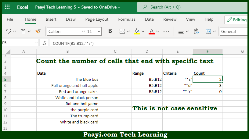
In this example, the goal is to count cells in the range B5:B16 that end with specific text, which is provided in column D. For convenience, the range B5:B16 is named data.
COUNTIF function
The simplest way to solve this problem is with the COUNTIF function and a wildcard. COUNTIF supports three wildcards that can be used in the criteria argument: question mark (?), asterisk(*), or tilde (~). A question mark (?) matches any one character and an asterisk (*) matches zero or more characters of any kind. The tilde (~) is an escape character to match literal wildcards that may appear in data. In this example, we mainly use an asterisk (*). To count cells in a range that end with «apple» you can use a formula like this:
=COUNTIF(range,"*apple) // end with "apple"
In the worksheet shown, we use the criteria in column D directly like this:
=COUNTIF(data,D5)
As the formula is copied down, COUNTIF returns the count of cells in data (B5:B16) that end with the text seen in D5:D8, which already includes the wildcard(s) needed. Notice that COUNTIF is not case-sensitive. Cell D6 contains a lowercase «y», yet COUNTIFS happily matches the uppercase «Y»s in B5:B16.
Below are the formulas in the worksheet, altered to include the criteria from column D directly:
=COUNTIF(data,"*R") // returns 3
=COUNTIF(data,"*y") // returns 2
=COUNTIF(data,"*002??-?") // returns 5
=COUNTIF(data,"*-?") // returns 12
Notice the last two formulas use both question mark (?) and asterisk (*) wildcards. The ? wildcard matches any one character, so you can use it to create criteria that is more specific than with just the * wildcard. Notice the hyphen (-) is hardcoded to make the pattern even more specific.
EXPLANATION
This tutorial shows how to count cells that end with a specific value using Excel formulas and VBA.
This tutorial provides two Excel methods that can be applied to count cells that end with a specific value by using the Excel COUNTIF function and the «*» criteria. The first method references to a cell for the specific value and in the second method the specific value is directly entered into the formula. The formulas count the cells from range (B8:B14) that end with «es».
This tutorial provides two VBA methods that can be applied to count cells that end with a specific value. The first method references to a cell for the specific value and in the second method the specific value is directly entered into the VBA code.
FORMULA (with value referenced to a cell)
=COUNTIF(range, «*»&value)
FORMULA (with value directly entered into the formula)
=COUNTIF(range, «*value»)
ARGUMENTS
range: The range of cells you want to count from.
value: The value that the cell ends with.
=COUNTIF(A2:A7,«*Apple«) // criteria within formula
=COUNTIF(A:A,«*»&C6) // criteria as a cell reference
A2:A7 & A:A = Ranges; C6 = Criteria; (a* = search «a» at start); (*b = search «b» at end)
Check below for a detailed explanation with pictures and how to use formulas in Excel and Google Sheets.
Count if cells end with a specific text in Excel
Count if cells end with a specific text in Excel
How to count cells end with a specific text in Excel?

COUNT IF CELLS END WITH A SPECIFIC TEXT — EXCEL FORMULA AND EXAMPLE
COUNT IF CELLS END WITH A SPECIFIC TEXT — EXCEL FORMULA AND EXAMPLE
-
=COUNTIF(A2:A7,«*Apple«) // criteria within formula
-
=COUNTIF(A:A,«*»&C6) // criteria as a cell reference
-
A2:A7 = data range
-
«*Apple« = criteria and must end with apple (non-case sensitive)
-
* asterisk explanation
-
a* = «a» at start
-
*b = «b» at end
-
-
Count if cells end with a specific text in Google Sheets
Count if cells end with a specific text in Google Sheets
How to count cells end with a specific text in Google Sheets?

COUNT IF CELLS END WITH A SPECIFIC TEXT — GOOGLE SHEETS FORMULA AND EXAMPLE
COUNT IF CELLS END WITH A SPECIFIC TEXT — GOOGLE SHEETS FORMULA AND EXAMPLE
-
=COUNTIF(A2:A6,«*Apple«) // criteria within formula
-
=COUNTIF(A:A,«*»&C6) // criteria as a cell reference
-
A2:A6 = data range
-
«*Apple« = criteria and must end with apple (non-case sensitive)
-
* asterisk explanation
-
a* = «a» at start
-
*b = «b» at end
-
-
Wild cards and regular expressions in Excel and Google Sheets
Wild cards and regular expressions in Excel and Google Sheets
![]() Wild cards and regular expressions
Wild cards and regular expressions
Other useful «COUNT FUNCTIONS: TEXT BASED CRITERIA» formulas in Excel and Google Sheets
- Count cells in the column that have the same first five characters
- Count cells over 10 characters
- Count cells that are not blank
- Count if cells contain a specific text
- Count cells that begin with a specific text
- Count cells that contain a specific text and ignore blank
- Count cells that contain errors
- Count if cells start with a specific text
- Count if cells end with a specific text
- Count the number of words in a cell
- Count the number of cells that have more than 5 characters words
- Count the number of occurrences of a text string in a range
- Count words in a range of cells and columns
- COUNTIF based on multiple criteria
Others Formulas
- Sum by month
- SUMIF cells if contains part of a text string
- Sum total sales based on quantity & price
- Combine date and time
- Convert 1-12 to month name
- Dynamic current date and time
- Count blank cell
- Count cell between two values
- Combine two or more cell
- Extract left before first space
- Extract the nth words in a text string
- Flip the first and last name
- SUMIF formulas and example
- SUMIFS formulas and example
- COUNTIF formulas and example
- IF formulas and example
- TEXT formulas and example
- CONVERT formulas and example
- Change the negative number to zero
- Change negative to positive numbers
- Calculate percentage changes for containing zero or negative values
Date and time functions
- Convert date to text
- Convert time to text
- Convert weekday string to number
- Combine two or more cells with a line break
- Combine two or more cells and transpose
Number based criteria
- Count cell between two values
- Count number of days between dates
Extract functions
- Get text between colons
- Transpose column to row
- Transpose row to column
Coming | Subscribe here for the custom Excel/Sheets formulas E-book (PDF) >
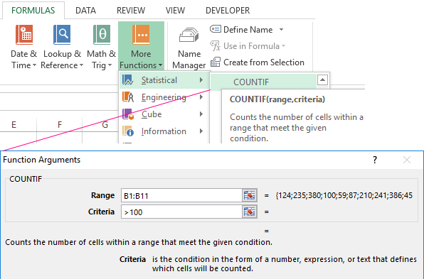
COUNTIF function
Use COUNTIF, one of the statistical functions, to count the number of cells that meet a criterion; for example, to count the number of times a particular city appears in a customer list.
In its simplest form, COUNTIF says:
-
=COUNTIF(Where do you want to look?, What do you want to look for?)
For example:
-
=COUNTIF(A2:A5,»London»)
-
=COUNTIF(A2:A5,A4)

COUNTIF(range, criteria)
|
Argument name |
Description |
|---|---|
|
range (required) |
The group of cells you want to count. Range can contain numbers, arrays, a named range, or references that contain numbers. Blank and text values are ignored. Learn how to select ranges in a worksheet. |
|
criteria (required) |
A number, expression, cell reference, or text string that determines which cells will be counted. For example, you can use a number like 32, a comparison like «>32», a cell like B4, or a word like «apples». COUNTIF uses only a single criteria. Use COUNTIFS if you want to use multiple criteria. |
Examples
To use these examples in Excel, copy the data in the table below, and paste it in cell A1 of a new worksheet.
|
Data |
Data |
|---|---|
|
apples |
32 |
|
oranges |
54 |
|
peaches |
75 |
|
apples |
86 |
|
Formula |
Description |
|
=COUNTIF(A2:A5,»apples») |
Counts the number of cells with apples in cells A2 through A5. The result is 2. |
|
=COUNTIF(A2:A5,A4) |
Counts the number of cells with peaches (the value in A4) in cells A2 through A5. The result is 1. |
|
=COUNTIF(A2:A5,A2)+COUNTIF(A2:A5,A3) |
Counts the number of apples (the value in A2), and oranges (the value in A3) in cells A2 through A5. The result is 3. This formula uses COUNTIF twice to specify multiple criteria, one criteria per expression. You could also use the COUNTIFS function. |
|
=COUNTIF(B2:B5,»>55″) |
Counts the number of cells with a value greater than 55 in cells B2 through B5. The result is 2. |
|
=COUNTIF(B2:B5,»<>»&B4) |
Counts the number of cells with a value not equal to 75 in cells B2 through B5. The ampersand (&) merges the comparison operator for not equal to (<>) and the value in B4 to read =COUNTIF(B2:B5,»<>75″). The result is 3. |
|
=COUNTIF(B2:B5,»>=32″)-COUNTIF(B2:B5,»<=85″) |
Counts the number of cells with a value greater than (>) or equal to (=) 32 and less than (<) or equal to (=) 85 in cells B2 through B5. The result is 1. |
|
=COUNTIF(A2:A5,»*») |
Counts the number of cells containing any text in cells A2 through A5. The asterisk (*) is used as the wildcard character to match any character. The result is 4. |
|
=COUNTIF(A2:A5,»?????es») |
Counts the number of cells that have exactly 7 characters, and end with the letters «es» in cells A2 through A5. The question mark (?) is used as the wildcard character to match individual characters. The result is 2. |
Common Problems
|
Problem |
What went wrong |
|---|---|
|
Wrong value returned for long strings. |
The COUNTIF function returns incorrect results when you use it to match strings longer than 255 characters. To match strings longer than 255 characters, use the CONCATENATE function or the concatenate operator &. For example, =COUNTIF(A2:A5,»long string»&»another long string»). |
|
No value returned when you expect a value. |
Be sure to enclose the criteria argument in quotes. |
|
A COUNTIF formula receives a #VALUE! error when referring to another worksheet. |
This error occurs when the formula that contains the function refers to cells or a range in a closed workbook and the cells are calculated. For this feature to work, the other workbook must be open. |
Best practices
|
Do this |
Why |
|---|---|
|
Be aware that COUNTIF ignores upper and lower case in text strings. |
|
|
Use wildcard characters. |
Wildcard characters —the question mark (?) and asterisk (*)—can be used in criteria. A question mark matches any single character. An asterisk matches any sequence of characters. If you want to find an actual question mark or asterisk, type a tilde (~) in front of the character. For example, =COUNTIF(A2:A5,»apple?») will count all instances of «apple» with a last letter that could vary. |
|
Make sure your data doesn’t contain erroneous characters. |
When counting text values, make sure the data doesn’t contain leading spaces, trailing spaces, inconsistent use of straight and curly quotation marks, or nonprinting characters. In these cases, COUNTIF might return an unexpected value. Try using the CLEAN function or the TRIM function. |
|
For convenience, use named ranges |
COUNTIF supports named ranges in a formula (such as =COUNTIF(fruit,»>=32″)-COUNTIF(fruit,»>85″). The named range can be in the current worksheet, another worksheet in the same workbook, or from a different workbook. To reference from another workbook, that second workbook also must be open. |
Note: The COUNTIF function will not count cells based on cell background or font color. However, Excel supports User-Defined Functions (UDFs) using the Microsoft Visual Basic for Applications (VBA) operations on cells based on background or font color. Here is an example of how you can Count the number of cells with specific cell color by using VBA.
Need more help?
You can always ask an expert in the Excel Tech Community or get support in the Answers community.

See also
COUNTIFS function
IF function
COUNTA function
Overview of formulas in Excel
IFS function
SUMIF function
Need more help?
Want more options?
Explore subscription benefits, browse training courses, learn how to secure your device, and more.
Communities help you ask and answer questions, give feedback, and hear from experts with rich knowledge.
- All articles
- COUNT
- Count cells that end with
While working with Excel, we are able to count values in a data set based on a given criteria by using the COUNTIF function. COUNTIF returns the number of values in a specified range based on a given condition. This step by step tutorial will assist all levels of Excel users in counting values that end with a specific text or character.
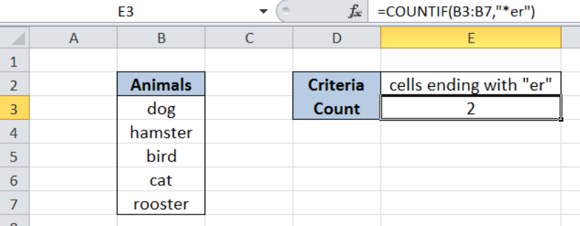 Figure 1. Final result: Count cells that end with “er”
Final formula: =COUNTIF(B3:B7,"*er")
Syntax of COUNTIF Function
=COUNTIF(range,criteria)
Parameters:
- range – the data range that will be evaluated using the criteria
- criteria – the criteria or condition that determines which cells will be counted
Setting up Our Data
Our table contains a list of Animals (column B). Cell E2 contains the criteria that we want to apply which is cells ending with “er”. In cell E3, the count based on the given criteria will be recorded.
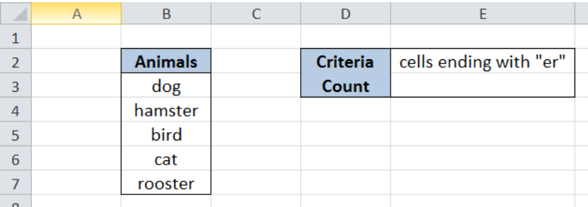 Figure 2. Sample data to count cells that end with “er”
Count cells that end with “er”
In order to determine the number of cells that end with “er”, we follow these steps:
Step 1. Select cell E3
Step 2. Enter the formula: =COUNTIF(B3:B7,"*er")
Step 3: Press ENTER
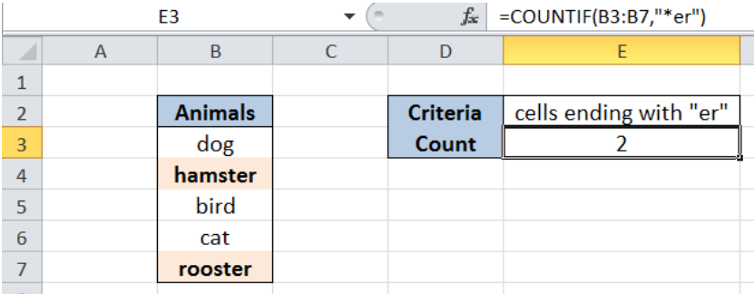 Figure 3. Using COUNTIF and asterisk “*” to count cells that end with “er”
Our range for the COUNTIF function is the range B3:B7 which contains our data for “Animals”. The criteria is “*er” which means that we want to count the animals whose names end with “er”. The asterisk “*” is a wildcard in Excel and it means that there could be any number of characters before “er”.
As a result, our formula returns 2, which corresponds to two values that end with “er”: hamster and rooster.
Most of the time, the problem you will need to solve will be more complex than a simple application of a formula or function. If you want to save hours of research and frustration, try our live Excelchat service! Our Excel Experts are available 24/7 to answer any Excel question you may have. We guarantee a connection within 30 seconds and a customized solution within 20 minutes.
Did this post not answer your question? Get a
solution from
connecting
with the expert.
Another blog reader asked this question today on Excelchat:

Debug the code (ran in vba) Dim arr(6 To 14, 3 To 11, 0 To 10) Dim arr1(6 To 14, 3 To 11, 0 To 10) Private Sub CommandButton1_Click() removecommments populatearray attempts = 1 Do While Not (complete() Or attempts > 15) parsegrid putcomments Sheet12.Cells(2, 7).Value = attempts attempts = attempts + 1 Loop End Sub Function complete() As Boolean emptycells = 0 For r = 6 To 14 For c = 3 To 11 If Sheet1.Cells(r, c).Value = «» Then emptycells = emptycells + 1 End If Next Next If emptycells <> 0 Then complete = True Else complete = False End If Sheet1.Cells(1, 7).Value = emptycells End Function Function parsegrid() For r = six To 14 For c = three To 11 zx = populateprobables(r, c) Next Next putvalues End Function Function populateprobables(ByVal rx As Integer, ByVal ry As String) As Variant If Sheet1.Cells(rx, ry).Value <> «» Then arr1(rx, ry, 0) = Sheet1.Cells(rx, ry).Value Else For cc = 3 To 11 If Sheet1.Cells(rx, cc).Value <> «» Then arr1(rx, ry, Sheet1.Cells(rx, cc).Value) = 0 End If Next For rr = 6 To 14 If Sheet1.Cells(rr, ry).Value <> «» Then arr1(rx, ry, Sheet1.Cells(rr, ry).Value) = 0 End If Next For cc = Application.WorksheetFunction.RoundDown(ry / 3, 0) * 3 To (Application.WorksheetFunction.RoundDown(ry / 3, 0) * 3) + 2 For rr = Application.WorksheetFunction.RoundDown(rx / 3, 0) * 3 To (Application.WorksheetFunction.RoundDown(rx / 3, 0) * 3) + 2 If Sheet1.Cells(rr, cc).Value <> «» Then arr1(rx, ry, Sheet1.Cells(rr, cc).Value) = 0 End If Next Next End If End Function Function putvalues() For r = 6 To 14 For c = 3 To 11 Count = 0 For x = 1 To 10 If arr1(r, c, x) <> 0 Then Count = Count + 1 thevalue = arr1(r, c, x) End If Next If Count = 1 Then arr1(r, c, 0) = thevalue Sheet1.Cells(r, c).Value = thevalue End If Next Next End Function Function populatearray() For r = 6 To 14 For c = 3 To 11 For x = 1 To 9 arr1(r, c, x) = x Next Next End Function Function putcomments() For r = 6 To 14 For c = 3 To 11 arrtxt = «» If arr1(r, c, 0) = 0 Then For x = 1 To 9 If arr1(r, c, x) <> 0 Then arrtxt = arrtxt & «-» & arr1(r, c, x) End If Next If Sheet1.Cells(r, c).Comment Is Nothing Then Else Sheet1.Cells(r, c).Comment.Delete End If Sheet1.Cells(r, c).AddComment («values possible are» & arrtxt) Sheet1.Cells(r, c).Comment.Visible = False End If Next Next End Function Function removecomments() For r = 6 To 14 For c = 3 To 11 If Sheet1.Cells(r, c).Comment Is Nothing Then Else Sheet1.Cells(r, c).Comment.Delete End If Sheet1.Cells(1, 7).Value = «» Sheet1.Cells(2, 7).Value = «» Next Next End Function Private Sub CommandButton2_Click() removecomments End Sub
An Excelchat Expert solved this problem in 17 mins!

The following code has errors when it runs. I need to fix the code so that there are no errors and the array shown in the worksheet fills correctly (sudoku!) Dim arr(6 To 14, 3 To 11, 0 To 10) Dim arr1(6 To 14, 3 To 11, 0 To 10) Private Sub CommandButton1_Click() removecommments populatearray attempts = 1 Do While Not (complete() Or attempts > 15) parsegrid putcomments Sheet12.Cells(2, 7).Value = attempts attempts = attempts + 1 Loop End Sub Function complete() As Boolean emptycells = 0 For r = 6 To 14 For c = 3 To 11 If Sheet1.Cells(r, c).Value = «» Then emptycells = emptycells + 1 End If Next Next If emptycells <> 0 Then complete = True Else complete = False End If Sheet1.Cells(1, 7).Value = emptycells End Function Function parsegrid() For r = six To 14 For c = three To 11 zx = populateprobables(r, c) Next Next putvalues End Function Function populateprobables(ByVal rx As Integer, ByVal ry As String) As Variant If Sheet1.Cells(rx, ry).Value <> «» Then arr1(rx, ry, 0) = Sheet1.Cells(rx, ry).Value Else For cc = 3 To 11 If Sheet1.Cells(rx, cc).Value <> «» Then arr1(rx, ry, Sheet1.Cells(rx, cc).Value) = 0 End If Next For rr = 6 To 14 If Sheet1.Cells(rr, ry).Value <> «» Then arr1(rx, ry, Sheet1.Cells(rr, ry).Value) = 0 End If Next For cc = Application.WorksheetFunction.RoundDown(ry / 3, 0) * 3 To (Application.WorksheetFunction.RoundDown(ry / 3, 0) * 3) + 2 For rr = Application.WorksheetFunction.RoundDown(rx / 3, 0) * 3 To (Application.WorksheetFunction.RoundDown(rx / 3, 0) * 3) + 2 If Sheet1.Cells(rr, cc).Value <> «» Then arr1(rx, ry, Sheet1.Cells(rr, cc).Value) = 0 End If Next Next End If End Function Function putvalues() For r = 6 To 14 For c = 3 To 11 Count = 0 For x = 1 To 10 If arr1(r, c, x) <> 0 Then Count = Count + 1 thevalue = arr1(r, c, x) End If Next If Count = 1 Then arr1(r, c, 0) = thevalue Sheet1.Cells(r, c).Value = thevalue End If Next Next End Function Function populatearray() For r = 6 To 14 For c = 3 To 11 For x = 1 To 9 arr1(r, c, x) = x Next Next End Function Function putcomments() For r = 6 To 14 For c = 3 To 11 arrtxt = «» If arr1(r, c, 0) = 0 Then For x = 1 To 9 If arr1(r, c, x) <> 0 Then arrtxt = arrtxt & «-» & arr1(r, c, x) End If Next If Sheet1.Cells(r, c).Comment Is Nothing Then Else Sheet1.Cells(r, c).Comment.Delete End If Sheet1.Cells(r, c).AddComment («values possible are» & arrtxt) Sheet1.Cells(r, c).Comment.Visible = False End If Next Next End Function Function removecomments() For r = 6 To 14 For c = 3 To 11 If Sheet1.Cells(r, c).Comment Is Nothing Then Else Sheet1.Cells(r, c).Comment.Delete End If Sheet1.Cells(1, 7).Value = «» Sheet1.Cells(2, 7).Value = «» Next Next End Function Private Sub CommandButton2_Click() removecomments End Sub
An Excelchat Expert solved this problem in 21 mins!

I have formatted a column with text not number so that I can enter 0 before value. And my column fill with hundreds of cells with numbers and I want to count the number of cells fill with numbers. I applied the formula =count(A1:A200) but results came 0. Please help in this regards.
An Excelchat Expert solved this problem in 26 mins!
Subscribe to Excelchat.co
Get updates on helpful Excel topics
Did this post not answer your question?
Get a solution from connecting with the expert
Another blog reader asked this question today on Excelchat:
Debug the code (ran in vba) Dim arr(6 To 14, 3 To 11, 0 To 10) Dim arr1(6 To 14, 3 To 11, 0 To 10) Private Sub CommandButton1_Click() removecommments populatearray attempts = 1 Do While Not (complete() Or attempts > 15) parsegrid putcomments Sheet12.Cells(2, 7).Value = attempts attempts = attempts + 1 Loop End Sub Function complete() As Boolean emptycells = 0 For r = 6 To 14 For c = 3 To 11 If Sheet1.Cells(r, c).Value = «» Then emptycells = emptycells + 1 End If Next Next If emptycells <> 0 Then complete = True Else complete = False End If Sheet1.Cells(1, 7).Value = emptycells End Function Function parsegrid() For r = six To 14 For c = three To 11 zx = populateprobables(r, c) Next Next putvalues End Function Function populateprobables(ByVal rx As Integer, ByVal ry As String) As Variant If Sheet1.Cells(rx, ry).Value <> «» Then arr1(rx, ry, 0) = Sheet1.Cells(rx, ry).Value Else For cc = 3 To 11 If Sheet1.Cells(rx, cc).Value <> «» Then arr1(rx, ry, Sheet1.Cells(rx, cc).Value) = 0 End If Next For rr = 6 To 14 If Sheet1.Cells(rr, ry).Value <> «» Then arr1(rx, ry, Sheet1.Cells(rr, ry).Value) = 0 End If Next For cc = Application.WorksheetFunction.RoundDown(ry / 3, 0) * 3 To (Application.WorksheetFunction.RoundDown(ry / 3, 0) * 3) + 2 For rr = Application.WorksheetFunction.RoundDown(rx / 3, 0) * 3 To (Application.WorksheetFunction.RoundDown(rx / 3, 0) * 3) + 2 If Sheet1.Cells(rr, cc).Value <> «» Then arr1(rx, ry, Sheet1.Cells(rr, cc).Value) = 0 End If Next Next End If End Function Function putvalues() For r = 6 To 14 For c = 3 To 11 Count = 0 For x = 1 To 10 If arr1(r, c, x) <> 0 Then Count = Count + 1 thevalue = arr1(r, c, x) End If Next If Count = 1 Then arr1(r, c, 0) = thevalue Sheet1.Cells(r, c).Value = thevalue End If Next Next End Function Function populatearray() For r = 6 To 14 For c = 3 To 11 For x = 1 To 9 arr1(r, c, x) = x Next Next End Function Function putcomments() For r = 6 To 14 For c = 3 To 11 arrtxt = «» If arr1(r, c, 0) = 0 Then For x = 1 To 9 If arr1(r, c, x) <> 0 Then arrtxt = arrtxt & «-» & arr1(r, c, x) End If Next If Sheet1.Cells(r, c).Comment Is Nothing Then Else Sheet1.Cells(r, c).Comment.Delete End If Sheet1.Cells(r, c).AddComment («values possible are» & arrtxt) Sheet1.Cells(r, c).Comment.Visible = False End If Next Next End Function Function removecomments() For r = 6 To 14 For c = 3 To 11 If Sheet1.Cells(r, c).Comment Is Nothing Then Else Sheet1.Cells(r, c).Comment.Delete End If Sheet1.Cells(1, 7).Value = «» Sheet1.Cells(2, 7).Value = «» Next Next End Function Private Sub CommandButton2_Click() removecomments End Sub
An Excelchat Expert solved this problem in 17 mins!
The following code has errors when it runs. I need to fix the code so that there are no errors and the array shown in the worksheet fills correctly (sudoku!) Dim arr(6 To 14, 3 To 11, 0 To 10) Dim arr1(6 To 14, 3 To 11, 0 To 10) Private Sub CommandButton1_Click() removecommments populatearray attempts = 1 Do While Not (complete() Or attempts > 15) parsegrid putcomments Sheet12.Cells(2, 7).Value = attempts attempts = attempts + 1 Loop End Sub Function complete() As Boolean emptycells = 0 For r = 6 To 14 For c = 3 To 11 If Sheet1.Cells(r, c).Value = «» Then emptycells = emptycells + 1 End If Next Next If emptycells <> 0 Then complete = True Else complete = False End If Sheet1.Cells(1, 7).Value = emptycells End Function Function parsegrid() For r = six To 14 For c = three To 11 zx = populateprobables(r, c) Next Next putvalues End Function Function populateprobables(ByVal rx As Integer, ByVal ry As String) As Variant If Sheet1.Cells(rx, ry).Value <> «» Then arr1(rx, ry, 0) = Sheet1.Cells(rx, ry).Value Else For cc = 3 To 11 If Sheet1.Cells(rx, cc).Value <> «» Then arr1(rx, ry, Sheet1.Cells(rx, cc).Value) = 0 End If Next For rr = 6 To 14 If Sheet1.Cells(rr, ry).Value <> «» Then arr1(rx, ry, Sheet1.Cells(rr, ry).Value) = 0 End If Next For cc = Application.WorksheetFunction.RoundDown(ry / 3, 0) * 3 To (Application.WorksheetFunction.RoundDown(ry / 3, 0) * 3) + 2 For rr = Application.WorksheetFunction.RoundDown(rx / 3, 0) * 3 To (Application.WorksheetFunction.RoundDown(rx / 3, 0) * 3) + 2 If Sheet1.Cells(rr, cc).Value <> «» Then arr1(rx, ry, Sheet1.Cells(rr, cc).Value) = 0 End If Next Next End If End Function Function putvalues() For r = 6 To 14 For c = 3 To 11 Count = 0 For x = 1 To 10 If arr1(r, c, x) <> 0 Then Count = Count + 1 thevalue = arr1(r, c, x) End If Next If Count = 1 Then arr1(r, c, 0) = thevalue Sheet1.Cells(r, c).Value = thevalue End If Next Next End Function Function populatearray() For r = 6 To 14 For c = 3 To 11 For x = 1 To 9 arr1(r, c, x) = x Next Next End Function Function putcomments() For r = 6 To 14 For c = 3 To 11 arrtxt = «» If arr1(r, c, 0) = 0 Then For x = 1 To 9 If arr1(r, c, x) <> 0 Then arrtxt = arrtxt & «-» & arr1(r, c, x) End If Next If Sheet1.Cells(r, c).Comment Is Nothing Then Else Sheet1.Cells(r, c).Comment.Delete End If Sheet1.Cells(r, c).AddComment («values possible are» & arrtxt) Sheet1.Cells(r, c).Comment.Visible = False End If Next Next End Function Function removecomments() For r = 6 To 14 For c = 3 To 11 If Sheet1.Cells(r, c).Comment Is Nothing Then Else Sheet1.Cells(r, c).Comment.Delete End If Sheet1.Cells(1, 7).Value = «» Sheet1.Cells(2, 7).Value = «» Next Next End Function Private Sub CommandButton2_Click() removecomments End Sub
An Excelchat Expert solved this problem in 21 mins!
I have formatted a column with text not number so that I can enter 0 before value. And my column fill with hundreds of cells with numbers and I want to count the number of cells fill with numbers. I applied the formula =count(A1:A200) but results came 0. Please help in this regards.
An Excelchat Expert solved this problem in 26 mins!
Post your problem and you’ll get expert help in seconds
Your message must be at least 40 characters
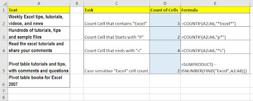
In this article, we will learn How to Count Cells That Contain Specific Text in Excel.
What is COUNTIFS with criteria ?
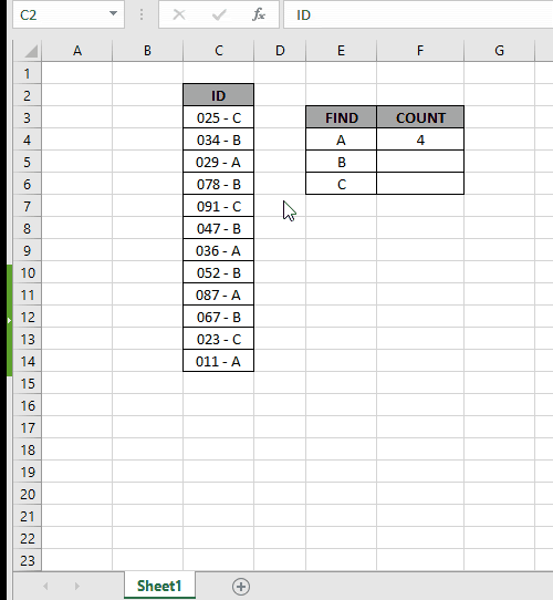
In simple words, while working with table values, sometimes we need to count the values which ends with a specific text or pattern. Example if we need to find the count of a certain ID which ends with a certain pattern. Criteria inside the formula executed using the operators. Let’s see the formula and example to illustrate the formula
How to solve the problem ?
For this article we will be required to use the COUNTIF function. Now we will make a formula out of the function. Here we are given some values in a range and specific text values as criteria. We need to count the values where the formula includes all the values which ends with the given text or pattern
Generic formula with hardcoded text:
range : values given in as range
* : wildcards which find any number of characters
text : given text or pattern to look for. Use text directly in the formula or else if you are using cell reference for the text use the other formula shown below.
Generic formula with text in reference cell:
= COUNTIF ( range, «*» & A1 & «*» )
A1 : text in A1 cell
& : operator to concatenate to «*text*»
Example:
All of these might be confusing to understand. So, let’s test this formula via running it on the example shown below. Here we have the ID records and we need to find the IDs which ends with A category.
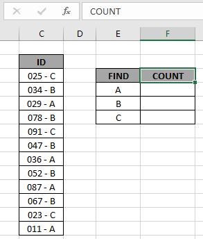
Here to find the A category IDs, will be using the * (asterisk) wildcard in the formula. * (asterisk) wildcard finds any number of characters within lookup value.
Use the formula:
OR
Explanation:
- COUNTIF function count the cells given criteria
- Criteria is given in using * (asterisk) wildcard to look for value which has any number of characters.
- & operator concatenate the two values where it lays
- «*» & E4 : criteria, formula checks each cell and returns only the cells which satisfies the criteria
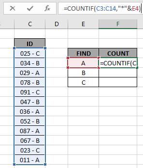
Here the range is given as array reference and pattern is given as cell reference. Press Enter to get the count.
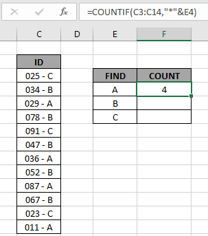
As you can see the total values which ends with value A comes out to be 4.
Now copy the formula in other cells using the drag down option or using the shortcut key Ctrl + D as shown below.
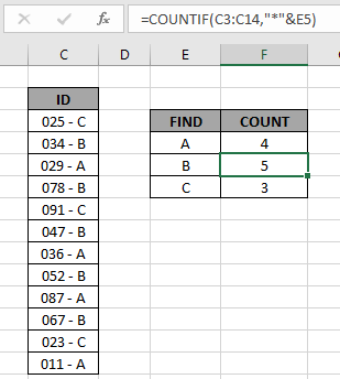
As you can see all the different category count of IDs is there.
You can check which values end with a specific pattern in range using the excel filter option. Apply the filter to the ID header and click the arrow button which appears. Follow the steps as shown below.
Steps:
- Select the ID header cell. Apply filter using shortcut Ctrl + Shift + L
- Click the arrow which appeared as a filter option.
- Deselect (Select All) option.
- Now search in search box using the * (asterisk) wildcard.
- Type *A in the search box and select the required values or select the (Select All search result) option as shown in the above gif.
As you can see in the above gif all the 4 values which match the given pattern. This also means the formula works fine to get the count of these values
Alternate COUNTIF formula with asterisk (*) wildcard.
To count all cell that contain “ExcelTip” in range A1:A10, we will write this formula:
=COUNTIF(A1:A10,”*ExcelTip*”)
To count all cells that start with “A” write this formula
=COUNTIF(A1:A10,”a*”)
To Count Cell that ends with “etc” write this COUNTIF formula
=COUNTIF(A1:A10,”*etc”)
Since COUNTIF is not case sensitive. It counts all cells that contain given text, irrespective of their case.
Here are all the observational notes using the formula in Excel
Notes :
- The formula only works with numbers and text both
- Operators like equals to ( = ), less than equal to ( <= ), greater than ( > ) or not equals to ( <> ) can be performed within functions applied with numbers only.
Hope this article about How to Count Cells That Contain Specific Text in Excel is explanatory. Find more articles on calculating values and related Excel formulas here. If you liked our blogs, share it with your friends on Facebook. And also you can follow us on Twitter and Facebook. We would love to hear from you, do let us know how we can improve, complement or innovate our work and make it better for you. Write to us at info@exceltip.com.
Related Articles :
How to use the SUMPRODUCT function in Excel: Returns the SUM after multiplication of values in multiple arrays in excel.
COUNTIFS with Dynamic Criteria Range : Count cells dependent on other cell values in Excel.
COUNTIFS Two Criteria Match : Count cells matching two different criteria on list in excel.
COUNTIFS With OR For Multiple Criteria : Count cells having multiple criteria match using the OR function.
The COUNTIFS Function in Excel : Count cells dependent on other cell values.
How to Use Countif in VBA in Microsoft Excel : Count cells using Visual Basic for Applications code.
How to use wildcards in excel : Count cells matching phrases using the wildcards in excel.
Popular Articles :
How to use the IF Function in Excel : The IF statement in Excel checks the condition and returns a specific value if the condition is TRUE or returns another specific value if FALSE.
How to use the VLOOKUP Function in Excel : This is one of the most used and popular functions of excel that is used to lookup value from different ranges and sheets.
How to use the SUMIF Function in Excel : This is another dashboard essential function. This helps you sum up values on specific conditions.
How to use the COUNTIF Function in Excel : Count values with conditions using this amazing function. You don’t need to filter your data to count specific values. Countif function is essential to prepare your dashboard.
In this article, you will learn how to COUNT various things in Mircosoft Excel using a single or combination of functions and its purpose in Microsoft Excel. You will also get to know how to count cells that end with specific text and see the generic
Count Cells that End With Specific Text in Microsoft Excel
The main purpose of this formula is to count the number of cells that end with the specific text. Here we will learn how to count the range of cells ending with the certain text in Microsoft Excel. That implies, with the help of a formula based on the COUNTIF function you can able to count the number of cells in a range that ends with the specific text. So, with the help of this formula, you can able to count the number of cells that have a certain text in the ending.
General Formula to COUNT Cells that End With Specific Text
=COUNTIF(rng,»*txt»)
The Explanation for the COUNT Cells that End With Specific Text
So we know that with the help of the given formula above you can able to count the number of cells that end with the specific text. Here we will learn how to count the range of cells ending with the certain text in Microsoft Excel. As we know that, the COUNTIF function is used to count the number of cells in the range that end with «a» by matching the content of each cell against the pattern «*a», which is supplied as the criteria. The «*» symbol r the asterisk is a wildcard in Microsoft Excel which means it can match any number of characters. It should be noted that the count of cells that match this pattern is returned as a number. So, with the help of this formula, you can able to count cells that end with a specific text.
Did this page help you?
|
The COUNTIF function is included in the group of statistical functions. It allows you to find the number of cells by a certain criterion. The COUNTIF function works with numeric and text values, as well as with dates.
Syntax and features of the function
First, let’s consider the arguments:
- Range – the group of values for analysis and counting (required).
- Criteria – the condition by which cells are to be counted (required).
The range of cells can include textual and numerical values, dates, arrays, and references to numbers. The function ignores empty cells.
A criterion can be a reference, a number, a text string, or an expression. The COUNTIF function only works with one criterion (by default). However, you can “force” it to analyze two criteria simultaneously.
Recommendations for the correct operation of the function:
- If the COUNTIF function refers to a range in another workbook, this workbook must be opened.
- The «Criteria» argument must be enclosed in quotation marks (except for references).
- The function does not take into account the letter case.
- When formulating a counting condition, you can use wildcard characters. The question mark «?» is any character. The asterisk «*» is any sequence of characters. For the formula to search for these signs directly, put a tilde (~) before them.
- For normal operation of the formula, cells with text values should not contain spaces or non-printable characters.
Countif function in Excel: examples
Let’s count the numerical values in one range. The counting condition is one criterion.
We have the following table:
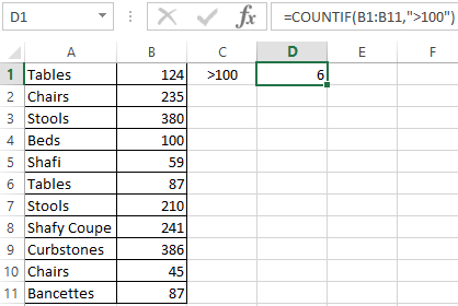
Count the number of cells with numbers greater than 100. Formula: =COUNTIF(B1:B11,»>100″). The range is В1:В11. The counting criterion is «>100». The result:
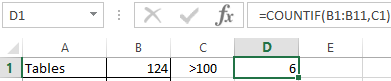
If the counting condition is entered in a separate cell, you can use the reference as a criterion:
Count the text values in one range. The search condition is one criterion. Formula: =COUNTIF(A1:A11,A3).
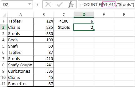
Or used reference inside the table:
In the second case, the cell reference was used as a criterion, result is the same – 2.
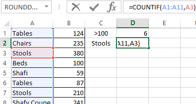
Formula with the wildcard character application: =COUNTIF(A1:A11,»Tab*»). To calculate the number of values ending in «и» and containing any number of characters: =COUNTIF(A1:A11,»*s»). We obtain:
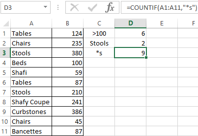
All names that end with a letter «s».
We use the search condition «not equal» in the COUNTIF.
Formula: =COUNTIF(A1:A11,»<>»&»Stools»). The operator «<>» means «not equal». The ampersand sign (&) is used to merge this operator and the “Stools” value.
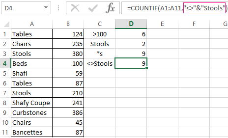
When you apply a reference, the formula will look like this:
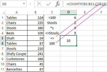
Often you need to perform the COUNTIF function in Excel by two criteria. In this way, you can significantly expand its capabilities. Let’s consider special cases of using the COUNTIF function in Excel and examples with two criteria.
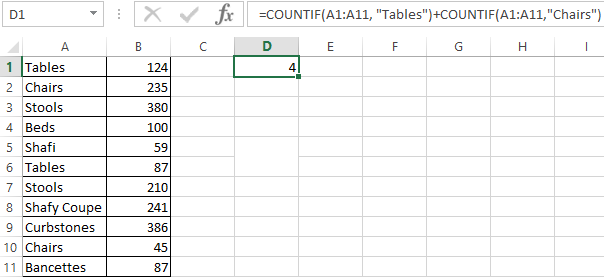
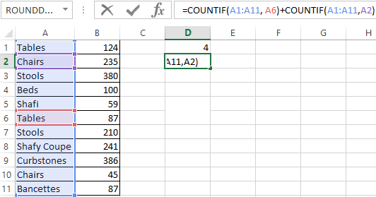
- Let’s count how many cells are contained in the » Tables » and » Chairs » text. Formula:
To specify several criteria, several COUNTIF phrases are used. They are united by the «+» operator.
- Criteria – cell references. Formula:
The function searches for » Tables » text in cell A1 and » Chairs » text – in cell A2 based on the criterion.
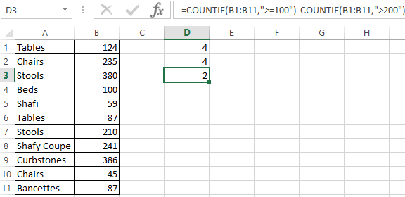
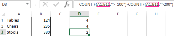
- Count the number of cells in B1:B11 range with a value greater than or equal to 100 and less than or equal to 200. Formula:
- Apply several ranges in the COUNTIF function. This is possible if the ranges are contiguous. It searches for values by two criteria in two columns simultaneously. If the ranges are not adjacent, then the COUNTIFS function is used.
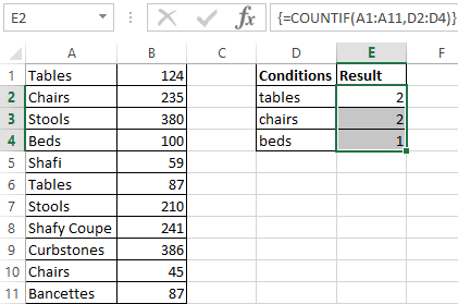
- When the criterion is a reference to a range of cells with conditions, the function returns the array. To enter a formula, you need to highlight as many cells as the range with criteria contains. After entering the arguments, simultaneously press Shift + Ctrl + Enter control key combination. Excel recognizes the formula of the array.
COUNTIF with two criteria in Excel is very often used for automated and efficient data handling. Therefore, an advanced user is highly recommended to carefully study all of the examples above.
Subtotal command and the countif function
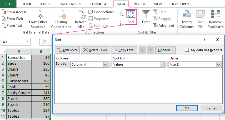
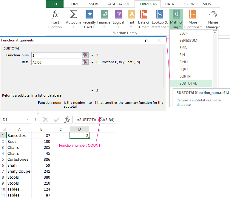
Count the number of goods sold in groups.
- First, sort the table so that the same values are close.
- The first argument of the formula “SUBTOTAL” – “Function number”. These are numbers from 1 to 11, indicating a statistical function for calculating the intermediate result. Counting the number of cells is carried out under number «2» (“COUNT”).
Download example COUNTIF in Excel
The formula has found the number of values for the «Chairs» group. For a large number of rows (more than a thousand), this combination of functions can be useful.
Maintenance Alert: Saturday, April 15th, 7:00pm-9:00pm CT. During this time, the shopping cart and information requests will be unavailable.
Intro to the COUNTIF Function in Excel
Categories: Excel®
Tags: countif function excel
Much of spreadsheet data is a collection of individual transactions or instances that don’t begin to offer meaning until they are organized and summarized in useful ways. Enter Excel’s handy COUNTIF function. When categories of data are mixed together, or if you wish to understand your data based on certain criteria, COUNTIF can help you sort the needed data from the rest or tally only information that falls into specified ranges. When combined with other functions, COUNTIF can become even more useful.
In this example we will show how to count data that falls within a certain range that we specify. Our table shows the monthly levels of contaminates present in an imaginary water sample taken over three years. We want to know how many months in that timeframe the levels were higher than 3.0 PPM (our “warning” level) and how many months the levels fell below 1.0 PPM.
To follow using our example, download Countif Function Excel. These examples apply to Excel 2007 and higher. Images were taken using Excel 2013 on Windows 7.

Count Cells That Match a Specified Criteria
The syntax for the COUNTIF function is COUNTIF(range, criteria) where
- The range argument defines the group of cells that you want counted.
- The criteria argument defines the circumstances under which a cell will be added to your count. The criteria can be a number, a cell reference, an expression or a text string.
In our example, we will place this example in E4:
=COUNTIF(B3:B43,”>3.0″)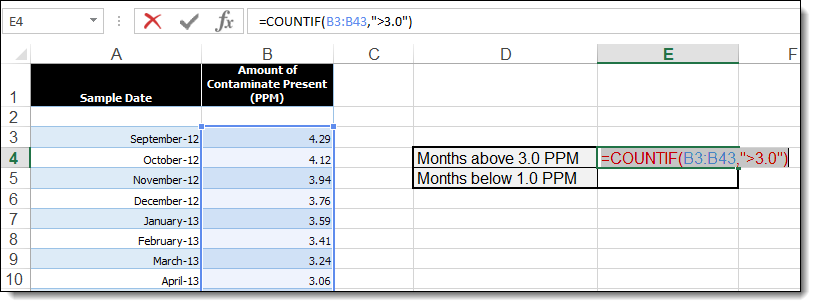
- B3:B43 tells the function to count cells in our “Amount” column
- “>3.0” tells the function to only count cells if they are greater than 3.0
In the same way, the formula that will go in E5 will be:
=COUNTIF(B3:B43,”<1.0″)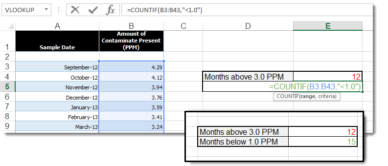
Use COUNTIF in Formulas
Now that we have COUNTIF working for us, we can combine it with other functions for even more data crunching. Using this same example, we can find out how many months fell between our high and low criteria by subtracting those results from the total. To do this we will combine the simple COUNT function with the functions we just specified to subtract them from the total number of months in our table:
=COUNT(B3:B43)-(COUNTIF(B3:B43,”>3.0″)+COUNTIF(B3:B43,”<1.0″))
- COUNT(B3:B43) gives us the total number of rows/months
- (COUNTIF(B3:B43,”>3.0″)+COUNTIF(B3:B43,”<1.0″)) adds together the number of rows/months over 3.0 and under 1.0 which are subtracted from the total number of rows.
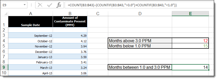
In this particular example we could have used the COUNTIFS function to specify a count of the rows between the two specified numbers. That formula would look like:
=COUNTIFS(B3:B43,”<3.0″,B3:B43,”>1.0″)
However, it does illustrate how you can use COUNTIF in formulas for data that isn’t numerical, for example, or if you are using a version older than Excel 2007.
Bonus Hint!
If you need to count data in a table that frequently changes – such as new rows added every month – then use a Named Range or a dynamic named range in the range argument. When your table changes, you only have to update the range in one place instead of each of the many places the range is used.
Here is a quick list of tasks that you can use COUNTIF to help you perform:
- Count cells that have specific numerical relationships such as between two numbers (as above), equal numbers, positive or negative numbers, numbers that are greater and less than a specified value or are specifically not
- Count cells that begin or end with a specified criteria
- Count cells that contain specific text or a certain number of characters
- Count matches in two ranges
- Find duplicates
What are some ways you have used COUNTIF to get the most out of your data?
PRYOR+ 7-DAYS OF FREE TRAINING
Courses in Customer Service, Excel, HR, Leadership,
OSHA and more. No credit card. No commitment. Individuals and teams.