
Excel for Microsoft 365 Excel 2021 Excel 2019 Excel 2016 Excel 2013 Excel 2010 Excel 2007 More…Less
To count numbers or dates that meet a single condition (such as equal to, greater than, less than, greater than or equal to, or less than or equal to), use the COUNTIF function. To count numbers or dates that fall within a range (such as greater than 9000 and at the same time less than 22500), you can use the COUNTIFS function. Alternately, you can use SUMPRODUCT too.
Example
Note: You’ll need to adjust these cell formula references outlined here based on where and how you copy these examples into the Excel sheet.
|
1 |
A |
B |
|---|---|---|
|
2 |
Salesperson |
Invoice |
|
3 |
Buchanan |
15,000 |
|
4 |
Buchanan |
9,000 |
|
5 |
Suyama |
8,000 |
|
6 |
Suyma |
20,000 |
|
7 |
Buchanan |
5,000 |
|
8 |
Dodsworth |
22,500 |
|
9 |
Formula |
Description (Result) |
|
10 |
=COUNTIF(B2:B7,»>9000″) |
The COUNTIF function counts the number of cells in the range B2:B7 that contain numbers greater than 9000 (4) |
|
11 |
=COUNTIF(B2:B7,»<=9000″) |
The COUNTIF function counts the number of cells in the range B2:B7 that contain numbers less than 9000 (4) |
|
12 |
=COUNTIFS(B2:B7,»>=9000″,B2:B7,»<=22500″) |
The COUNTIFS function (available in Excel 2007 and later) counts the number of cells in the range B2:B7 greater than or equal to 9000 and are less than or equal to 22500 (4) |
|
13 |
=SUMPRODUCT((B2:B7>=9000)*(B2:B7<=22500)) |
The SUMPRODUCT function counts the number of cells in the range B2:B7 that contain numbers greater than or equal to 9000 and less than or equal to 22500 (4). You can use this function in Excel 2003 and earlier, where COUNTIFS is not available. |
|
14 |
Date |
|
|
15 |
3/11/2011 |
|
|
16 |
1/1/2010 |
|
|
17 |
12/31/2010 |
|
|
18 |
6/30/2010 |
|
|
19 |
Formula |
Description (Result) |
|
20 |
=COUNTIF(B14:B17,»>3/1/2010″) |
Counts the number of cells in the range B14:B17 with a data greater than 3/1/2010 (3) |
|
21 |
=COUNTIF(B14:B17,»12/31/2010″) |
Counts the number of cells in the range B14:B17 equal to 12/31/2010 (1). The equal sign is not needed in the criteria, so it is not included here (the formula will work with an equal sign if you do include it («=12/31/2010»). |
|
22 |
=COUNTIFS(B14:B17,»>=1/1/2010″,B14:B17,»<=12/31/2010″) |
Counts the number of cells in the range B14:B17 that are between (inclusive) 1/1/2010 and 12/31/2010 (3). |
|
23 |
=SUMPRODUCT((B14:B17>=DATEVALUE(«1/1/2010»))*(B14:B17<=DATEVALUE(«12/31/2010»))) |
Counts the number of cells in the range B14:B17 that are between (inclusive) 1/1/2010 and 12/31/2010 (3). This example serves as a substitute for the COUNTIFS function that was introduced in Excel 2007. The DATEVALUE function converts the dates to a numeric value, which the SUMPRODUCT function can then work with. |
Need more help?
Want more options?
Explore subscription benefits, browse training courses, learn how to secure your device, and more.
Communities help you ask and answer questions, give feedback, and hear from experts with rich knowledge.
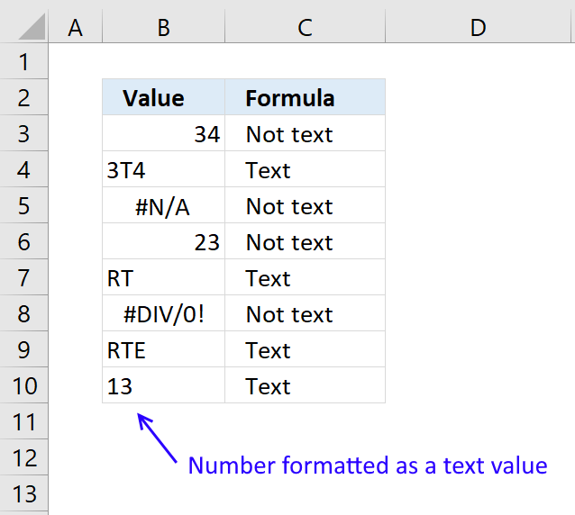
COUNTIF Not Blank Function
The COUNTIF not blank function counts non-blank cells within a range. The universal formula is “COUNTIF(range,”<>”&””)” or “COUNTIF(range,”<>”)”. This formula works with numbers, text, and date values. It also works with the logical operators like “<,” “>,” “=,” and so on.
Note: Alternatively, the COUNTA functionThe COUNTA function is an inbuilt statistical excel function that counts the number of non-blank cells (not empty) in a cell range or the cell reference. For example, cells A1 and A3 contain values but, cell A2 is empty. The formula “=COUNTA(A1,A2,A3)” returns 2.
read more can be used to count the non-blank cells.
Table of contents
- COUNTIF Not Blank Function
- How to Use COUNTIF Non-Blank Function?
- #1–Numerical Values
- #2–Text Values
- #3–Date Values
- The Characteristics of COUNTIF Not Blank Function
- Frequently Asked Questions
- Recommended Articles
- How to Use COUNTIF Non-Blank Function?
How to Use COUNTIF Non-Blank Function?
#1–Numerical Values
The steps to count non-empty cells with the help of the COUNTIF function are listed as follows:
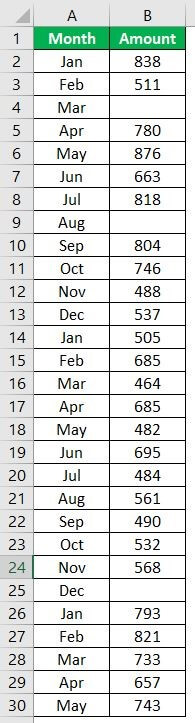
- In Excel, enter the following data containing both, the data cells and the empty cells.

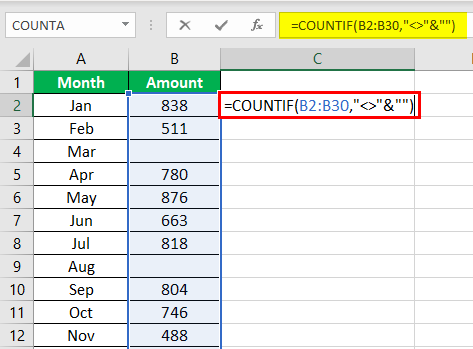
- Enter the following formula to count the data cells.
“=COUNTIF(range,”<>”&””)”
In the range argument, type B2:B30. Alternatively, select the range B2:B30 in the formula, as shown in the following image.

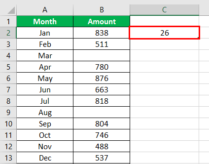
- Press the “Enter” key. The number of non-blank cells in the range B2:B30 appear in cell C2. The output is 26, as shown in the succeeding image.
This implies that there are 26 cells in the given range that contain a data value. This data can be a number, text, or any other value.

#2–Text Values
The steps to count non-empty cells within text values are listed as follows:
- Step 1: In Excel, enter the data as shown in the following image.
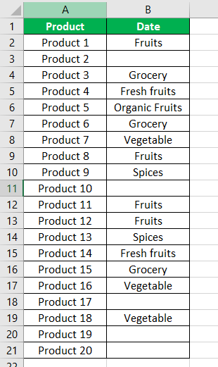
- Step 2: Select the range within which data needs to be checked for non-blank values. Enter the formula shown in the succeeding image.
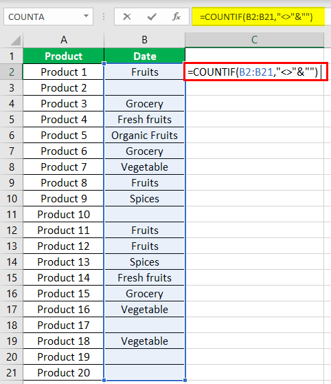
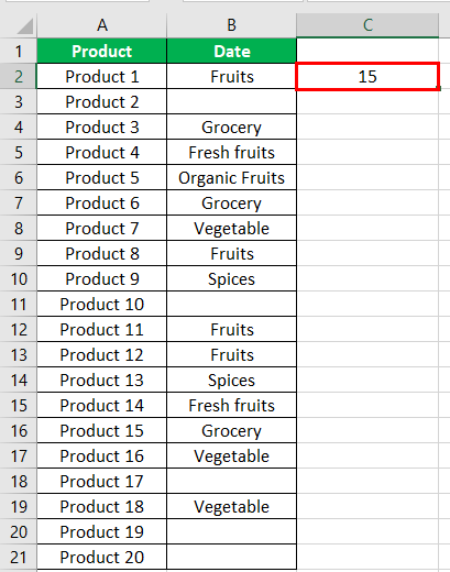
- Step 3: Press the “Enter” key. The number of non-blank cells in the range B2:B21 appear in cell C2. The output is 15, as shown in the succeeding image.
Hence, the COUNTIF not blank formula works with text values.
#3–Date Values
The steps to count non-empty cells, when the data consists of dates, are listed as follows:
- Step 1: In Excel, enter the data as shown in the following image. Select the range whose data needs to be checked for non-blank values. Enter the following formula.
“=COUNTIF(B2:B21,”<>”&””)”
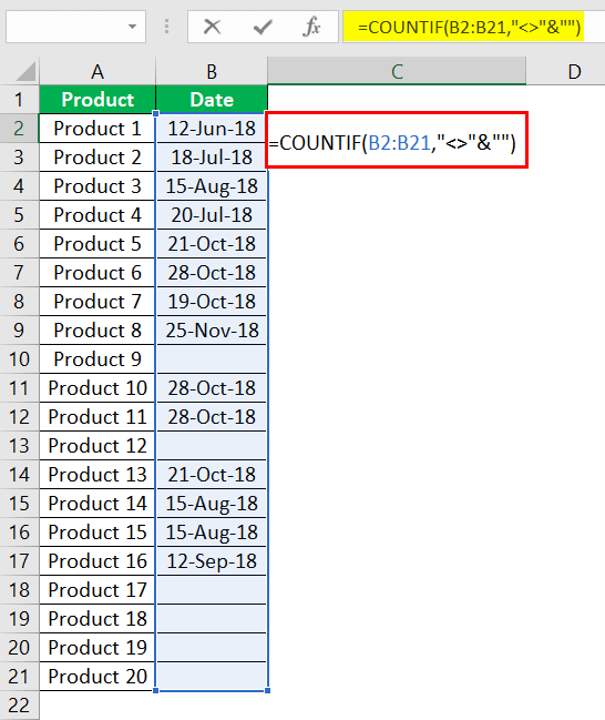
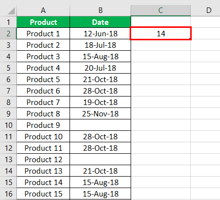
- Step 2: Press the “Enter” key. The number of non-blank cells in the range B2:B21 appear in cell C2. The output is 14, as shown in the succeeding image.
Hence, the COUNTIF not blank formula works with data that consists of date values.
The Characteristics of COUNTIF Not Blank Function
- It is case insensitive, implying that the output remains the same irrespective of whether the formula is entered in uppercase or lowercase.
- It works for data that consists of numbers, text, and date values.
- It works with greater than (>) and less than (<) operators.
- It is difficult to use the formula with long strings.
- The criteria (condition) must be specified within a pair of inverted commas to avoid errors.
Frequently Asked Questions
How is the COUNTIF formula used to count blanks?
The universal formula for counting blanks is stated as follows:
“COUNTIF(range,””)”
This formula works with all types of data values.
Note: Alternatively, the COUNTBLANK function can be used to count blank cells.
How does the COUNTIF function count the duplicate values?
The formula for counting the duplicate value is given as follows:
“COUNTIF(range,“duplicate value”)”
The “range” represents the range within which the duplicate values are to be counted. The “duplicate value” is the exact data value that is to be counted.
For example, to count the number of times the text “fruits” appears in the range A2:A10, we use “=COUNTIF(A2:A10,“fruits”).”
- The COUNTIF not blank function counts the non-blank cells within a given range.
- The generic formula of the COUNTIF not blank function is stated as–“COUNTIF (range,“<>”&””).”
- The criteria (condition) must be specified within a pair of inverted commas to avoid errors.
- The COUNTIF functionThe COUNTIF function in Excel counts the number of cells within a range based on pre-defined criteria. It is used to count cells that include dates, numbers, or text. For example, COUNTIF(A1:A10,”Trump”) will count the number of cells within the range A1:A10 that contain the text “Trump”
read more works for data that consists of numbers, text, and date values. - The COUNTIF formula gives the same output irrespective of whether the formula is entered in uppercase or lowercase.
Recommended Articles
This has been a guide to Excel COUNTIF not blank. Here we discuss how to use the COUNTIF function to count non-blank cells along with practical examples and a downloadable Excel template. You may learn more about Excel from the following articles –
- Not Equal in VBA
- COUNTIF with Multiple Criteria
- VLOOKUP Errors
- Use Not Equal to in Excel
- XML in Excel
In this example, the goal is to count cells in a range that are not blank (i.e. not empty). There are several ways to go about this task, depending on your needs. The article below explains different approaches.
COUNTA function
While the COUNT function only counts numbers, the COUNTA function counts both numbers and text. This means you can use COUNTA as a simple way to count cells that are not blank. In the example shown, the formula in F6 uses COUNTA like this:
=COUNTA(C5:C16) // returns 9
Since there are nine cells in the range C5:C16 that contain values, COUNTA returns 9. COUNTA is fully automatic, so there is nothing to configure.
COUNTIFS function
You can also use the COUNTIFS function to count cells that are not blank like this:
=COUNTIFS(C5:C16,"<>") // returns 9
The «<>» operator means «not equal to» in Excel, so this formula literally means count cells not equal to nothing. Because COUNTIFS can handle multiple criteria, we can easily extend this formula to count cells that are not empty in Group «A» like this:
=COUNTIFS(B5:B16,"A",C5:C16,"<>") // returns 4
The first range/criteria pair selects cells that are in Group A only. The second range/criteria pair selects cells that are not empty. The result from COUNTIFS is 4, since there are 4 cells in Group A that are not empty. You can swap the order of the range/criteria pairs with the same result.
See also: 50 examples of formula criteria.
SUMPRODUCT function
One problem with COUNTA and COUNTIFS is that they will also count empty strings («») returned by formulas as not blank, even though these cells are intended to be blank. For example, if A1 contains 21, this formula in B1 will return an empty string:
=IF(A1>30,"Overdue","")However, COUNTA and COUNTIFS will still count B1 as not empty. If you run into this problem, you can use the SUMPRODUCT function to count cells that are not blank like this:
=SUMPRODUCT(--(C5:C16<>""))

The expression C5:C16<>»» returns an array that contains 12 TRUE and FALSE values, and the double negative (—) converts the TRUE and FALSE values to 1s and 0s:
=SUMPRODUCT({1;1;0;1;1;0;1;1;1;0;1;1}) // returns 9
The result is 9 as before. But this formula will also ignore cells that contain formulas that return empty strings.
You can easily extend the logic used in SUMPRODUCT with other functions as needed. For example, the variant below uses the LEN function to count cells that have a length greater than zero:
=SUMPRODUCT(--(LEN(C5:C16)>0)) // returns 9
You can extend the formula to count cells that are not blank in Group A like this:
=SUMPRODUCT((LEN(C5:C16)>0)*(B5:B16="A"))
This is an example of using Boolean algebra in a formula. The double negative is no longer needed in this case because the math operation of multiplying the two arrays together automatically converts the TRUE and FALSE values to 1s and 0s:
=SUMPRODUCT({1;1;0;1;1;0;0;0;0;0;0;0}) // returns 4
The final result is 4, since there are four cells in Group A that are not blank in C5:C16.
Note: one reason the Boolean syntax above is useful is because you can drop the same logical expressions into a newer function like the FILTER function to extract cells that meet the same criteria. The SUMPRODUCT function is more versatile than RACON functions like COUNTIFS, SUMIFS, etc. and you will often see it used in formulas that solve tricky problems. You can read more about SUMPRODUCT here.
This formula will count only numbers <> 0, excluding blanks, error messages, etc. BUT it will not exclude the cells that display ###### (but really contain a number) if the reason for that is a column that is too narrow, or a negative date or time value.
=SUMPRODUCT(--ISNUMBER(A2:A200))-COUNTIF(A2:A200,0)
If you really want to avoid counting cells that display ####### when the underlying contents is a number not equal to zero, you will need to use a UDF to act on the Text property of the cell. In addition, narrowing or widening the column to produce that affect will not trigger a calculation event that would update the formula, so you need to somehow do that in order to ensure the formula results are correct.
That is why I added Application.Volatile to the code, but it is still possible to produce a situation where the result of the formula does not agree with the display in the range being checked, at least until the next calculation event takes place.
To enter this User Defined Function (UDF), alt-F11 opens the Visual Basic Editor.
Ensure your project is highlighted in the Project Explorer window.
Then, from the top menu, select Insert/Module and
paste the code below into the window that opens.
To use this User Defined Function (UDF), enter a formula like
=CountNumbersNEZero(A2:A200)
in some cell.
Option Explicit
Function CountNumbersNEZero(rg As Range) As Long
Application.Volatile
    Dim C As Range
    Dim L As Double
For Each C In rg
    If IsNumeric(C.Text) Then
        If C.Text <> 0 Then L = L + 1
    End If
Next C
CountNumbersNEZero = L
End Function
This is going to be a super simple post, here our aim is to find the number of cells that contain data, cells that are blank or empty should be excluded. The task is quite simple but the question becomes ‘how to do it?’. You know you want Excel to count a certain type of cells for you but if you find yourself wondering what to put in your sheets to get that count, you’re about to find out.
This tutorial will walk you through the usage of functions to count non-blank cells and at the end, we will also see a few functions to selectively count only the blank cells. So, without further ado, let’s jump right in.
 1")
Counting Cells That Are Not Blank
Here we are going to talk about three Excel functions that can help us to count non-blank cells from a range.
Using COUNTIF Function
The COUNTIF function counts the number of cells within a range that meet the given criteria. COUNTIF asks for the range from which it needs to count and the criteria according to which it needs to count. To count all the non-blank cells with COUNTIF we can make use of the following formula:
=COUNTIF(range,"<>")
Let’s try to understand this with an example. So, we have a dataset as shown below:
 2")
From this list of product discounts, we will aim to find how many products are discounted. In Excel’s terminology, this means – we are finding out how many non-blank cells there are in column D (the non-blank cells represent the discounts on products and the blank cells represent products with no discount).
We can easily accomplish this using the following COUNTIF formula:
=COUNTIF(D3:D14,"<>")
And our final result looks something like this.
 3")
Here, the formula has been fed with the range of column D (D3:D14). The criteria for searching column D is «<>» which is the indicator for non-blank cells («» for blank cells).
The COUNTIF function has counted 8 non-blank cells as the result. This tells us that in our dataset, there are 8 products on discount.
The COUNTIF function can be used for only one condition. For multiple conditions (e.g., non-blank cells and discount more than 20%), we can use the COUNTIFS function.
The next function we will use to count if not blank cells are present in a range is the COUNTA function.
Using COUNTA Function
By its nature, the COUNTA function counts the cells in a range that are not empty. It is a single argument function (in its simplest form) requiring just the range from which to count non-blank cells.
We will use it in our last example and simply add our range D3:D14 to the COUNTA function in this way:
=COUNTA(D3:D14)
We have the same results as the COUNTIF function i.e., 8 non-blank cells, with fewer arguments.
 4")
For the sole purpose of counting non-blank cells, the COUNTA function offers an easy, straightforward solution.
However, the COUNTA and COUNTIF functions will also count cells with space characters and formulas that return an empty string. This means that the functions will count cells that look blank but are not essentially blank.
Why is that a problem?
Technically, a space character or a formula that returns an empty string is very different from a blank cell. Although they look similar but technically they are two different things.
But since our purpose here is to count non-blank cells, so we might want the cells that appear blank to be counted as blank cells (technically, even though they are not blank). To accomplish this instead of using the COUNTIF or COUNTA functions it is better to use a SUMPRODUCT function. And this is what we are going to see in the next section.
Tip: If you are adamant about using the COUNTIF or COUNTA function for counting non-blank cells, another way around it would be to filter the data and get rid of the cells with hidden values. This will refine the results without the inclusion of faux blank cells. For now, we will move onto the SUMPRODUCT function.
Using SUMPRODUCT Function
The SUMPRODUCT returns the sum of the products of the supplied ranges or arrays. To count non-blank cells using SUMPRODUCT function we can use the below formula:
=SUMPRODUCT(--(C2:C13<>""))
Let’s try to understand the formula first and then we can compare it with the COUNTIF and COUNTA functions.
In the above formula, first of all, we are checking if the values in the range C2:C13 are equal to an empty string (nothing). This returns an array of boolean values like this –
=SUMPRODUCT(--({TRUE, TRUE, TRUE, FALSE, TRUE, TRUE, TRUE, TRUE, FALSE, TRUE, TRUE, TRUE}))
Now, since the SUMPRODUCT function cannot sum boolean values we are converting them to 0’s and 1’s by using the double-negatives. So, the formula gets further simplified to something like this –
=SUMPRODUCT({1, 1, 1, 0, 1, 1, 1, 1, 0, 1, 1, 1})
The SUMPRODUCT function adds all these 1’s and 0’s and returns the final result.
An important thing worth noting here is that the above formula does not treat space character as an empty string (nothing) so it will still be counted as a non-blank cell. To count them as blanks we can make use of the TRIM function and the final formula would look like this –
=SUMPRODUCT(--(TRIM(C2:C13)<>""))
Pro Tip: Instead of using the double negatives to convert boolean values to 1’s and 0’s we can also either add 0 to them or multiply them by 1 and our final result would still be the same.
Now, Let’s have the COUNTIF, COUNTA, and SUMPRODUCT functions side by side and analyze them:
 5")
What we can see from the serial numbering, is that there are 12 rows in our dataset. C5 is a blank cell that is correctly interpreted as blank cells by COUNTIF and COUNTA. It appears that there are 2 more blank cells (C8 containing a space character and C10 containing a formula that returns an empty string i.e., =»») in the range which means that there are 9 non-blank cells.
While the COUNTIF and COUNTA functions have treated C5 as a blank cell but they treat the other two C8 and C10 as non-blank cells and thus return 11 as the count.
On the other hand, the SUMPRODUCT based formula correctly identifies all such cells and hence returns 9 as the count of non-blank cells.
Recommended Reading: Counting Unique Values In Excel
Counting Blank Cells
Now is the turn for counting blank cells. We have ahead 2 very simple ways of counting empty cells with help of the COUNTBLANK and the COUNTIF function.
Using COUNTBLANK Function
The COUNTBLANK function, pretty self-explanatory, counts the number of empty/blank cells in a specified range. We will use the function plainly to get our results:
=COUNTBLANK(D3:D14)
 6")
We have inserted the range D3:D14 in the formula to see how many blank cells there are in column D which will tell us the number of products with no discount. The outcome of the COUNTBLANK function is «4» blank cells.
Using COUNTIF Function
As explained above, the COUNTIF function can be used for counting both, blank and non-blank cells. Now we will see how to use COUNTIF for counting blank cells.
To count blank cells the COUNTIF function can be used as:
=COUNTIF(D3:D14,"")
 7")
In the formula, which is made up of the range and criteria, we have swapped the criteria for counting non-blank cells (i.e., «<>») with the criteria for counting blank cells (i.e., «»). With the range specified as D3:D14, the COUNTIF function returns «4» blank cells as the result, indicating 4 undiscounted products.
At the end of this tutorial, we hope you won’t feel blank when trying to count if not blank and blank cells. We’re following up with more how-to’s as you read!
Содержание
- Count if and countif excel
- Table of contents
- 1. Use IF + COUNTIF to evaluate multiple conditions
- 1.1 Explaining formula in cell D3
- Step 1 — COUNTIF function syntax
- Step 2 — Populate COUNTIF function arguments
- Step 3 — Evaluate COUNTIF function
- Step 4 — IF function syntax
- Step 5 — Populate IF function arguments
- Step 6 — Evaluate IF function
- 2. Use IF + COUNTIF to evaluate multiple conditions and calculate different outcomes
- 2.1 Explaining formula
- Step 1 — Check if the value matches any of the conditions
- Step 2 — IF function
- Step 3 — Calculate the relative position of a lookup value
- Step 3 — Get value
- Step 4 — Add values
- Get Excel *.xlsx file
- Logic category
- Functions in this article
- Excel formula categories
- Excel categories
- 3 Responses to “Use IF + COUNTIF to evaluate multiple conditions”
- Leave a Reply
- How to comment
- Excel COUNTIF and COUNTIFS with OR logic
- Count cells with OR conditions in Excel
- Formula 1. COUNTIF + COUNTIF
- Formula 2. COUNTIF with array constant
- Formula 3. SUMPRODUCT
- Count cells with OR as well as AND logic
- Formula 1. COUNTIFS + COUNTIFS
- Formula 2. COUNTIFS with array constant
- Count cells with multiple OR conditions
- Count cells with 2 sets of OR conditions
- Count cells with multiple sets of OR conditions
- Practice workbook
- You may also be interested in
Count if and countif excel
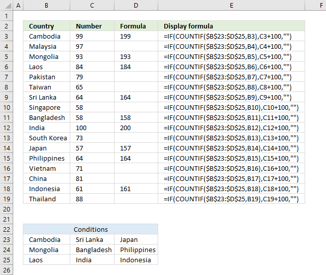
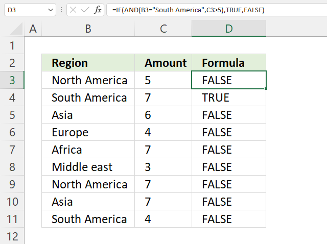
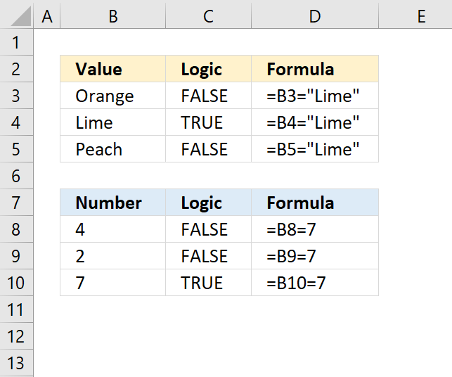
The image above demonstrates a formula that matches a value to multiple conditions, if the condition is met the formula takes the value in a corresponding cell on the same row and adds a given number.
Table of contents
The COUNTIF function allows you to construct a small IF formula that carries out plenty of logical expressions.
Combining the IF and COUNTIF functions also let you have more than 254 logical expressions and the effort to type the formula is minimal.
1. Use IF + COUNTIF to evaluate multiple conditions
The example shown in the above picture checks if the country in cell B3 is equal to one of the countries in cell range B23:D25.
In other words, the COUNTIF function counts how many times a specific value is found in a cell range.
If the value exists at least once in the cell range the IF function adds 100 to the value in C3. If FALSE the formula returns a blank.
1.1 Explaining formula in cell D3
Step 1 — COUNTIF function syntax
The COUNTIF function calculates the number of cells that is equal to a condition.
Step 2 — Populate COUNTIF function arguments
range — A reference to all conditions: $B$23:$D$25
criteria — The value to match.
Step 3 — Evaluate COUNTIF function
and returns 1. The criteria value is found once in the array (bolded).
Step 4 — IF function syntax
The IF function returns one value if the logical test is TRUE and another value if the logical test is FALSE.
IF(logical_test, [value_if_true], [value_if_false])
Step 5 — Populate IF function arguments
IF(logical_test, [value_if_true], [value_if_false])
logical_test — True or False, the numerical equivalents are TRUE — 1 and False — 0 (zero). 1, in this case, is equal to TRUE.
[value_if_true] — C3+100, add 100 to value in cell C3.
Step 6 — Evaluate IF function
IF(COUNTIF($B$23:$D$25, B3), C3+100, «»)
and returns 199 in cell D3.
2. Use IF + COUNTIF to evaluate multiple conditions and calculate different outcomes
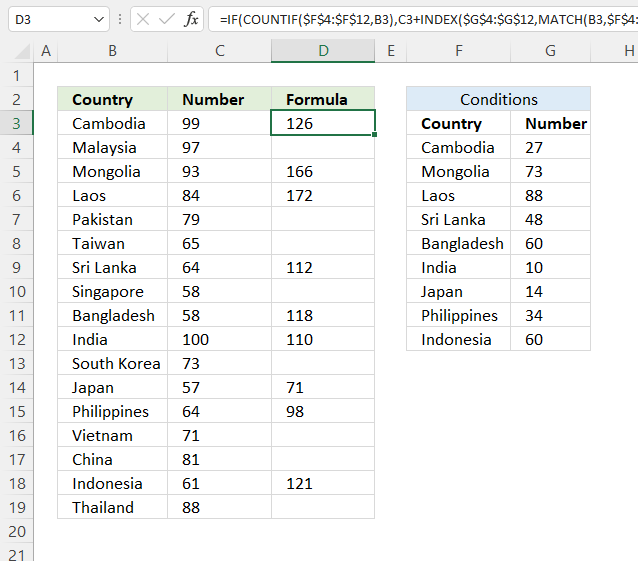
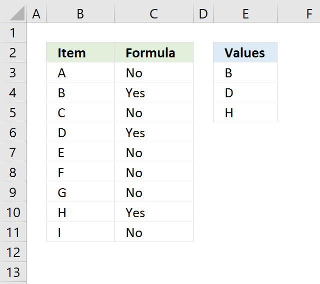
The image above demonstrates a formula in cell D3 that checks if the value in cell B3 matches any of the conditions specified in cell range F4:F12. If so, add the corresponding number in cell range G4:G12 to the number in cell C3.
Formula in cell D3:
2.1 Explaining formula
Step 1 — Check if the value matches any of the conditions
The COUNTIF function calculates the number of cells that is equal to a condition.
and returns 1. This means that there is one value that matches.
Step 2 — IF function
The IF function returns one value if the logical test is TRUE and another value if the logical test is FALSE.
IF(logical_test, [value_if_true], [value_if_false])
IF(COUNTIF($F$4:$F$12, B3), [value_if_true], [value_if_false])
IF(1, [value_if_true], [value_if_false])
[value_if_true] — C3+INDEX($G$4:$G$12, MATCH(B3, $F$4:$F$12,0))
Step 3 — Calculate the relative position of a lookup value
The MATCH function returns the relative position of an item in an array or cell reference that matches a specified value in a specific order.
MATCH(lookup_value, lookup_array, [match_type])
and returns 1. The lookup value is found at the first position in the array.
Step 3 — Get value
The INDEX function returns a value from a cell range, you specify which value based on a row and column number.
INDEX(array, [row_num], [column_num])
INDEX($G$4:$G$12, MATCH(B3, $F$4:$F$12,0))
Step 4 — Add values
The plus sign lets you add numbers in an Excel formula.
C3+INDEX($G$4:$G$12, MATCH(B3, $F$4:$F$12,0))
99 + 27 equals 126.
Get Excel *.xlsx file
Logic category
Functions in this article
Excel formula categories
Excel categories
3 Responses to “Use IF + COUNTIF to evaluate multiple conditions”
1. If item Count in Column-A have equal Count of the same item in corresponding Column-B, Result should be «Complete»
2. If item Count in Column-A have Count at least one in corresponding Column-B but less than Count in Column-A, Result should be «In progress»
3. If item Count in Column-A have no Count in corresponding Column-B, Result should be «Not Complete»
4. If there is no Count in Column-A and corresponding Column-B have no count, Result should be «Blank»
Please reply
If the marks of a student is less than 16 or his average is less than 50 he must be in D group.
How can i write this formula? Please write it for me
Please reply
If the marks of a student is less than 16 or his average is less than 50 he must be in D group.
How can i write this formula in table of contant? Please write it for me
Leave a Reply
How to add a formula to your comment
Insert your formula here.
Convert less than and larger than signs
Use html character entities instead of less than and larger than signs.
becomes >
How to add VBA code to your comment
[vb 1=»vbnet» language=»,»]
Put your VBA code here.
[/vb]
How to add a picture to your comment:
Upload picture to postimage.org or imgur
Paste image link to your comment.
Contact Oscar

You can contact me through this contact form
Источник
Excel COUNTIF and COUNTIFS with OR logic
 by Svetlana Cheusheva, updated on March 17, 2023
The tutorial explains how to use Excel’s COUNTIF and COUNTIFS functions to count cells with multiple OR conditions, e.g. if a cell contains X, Y or Z.
As everyone knows, Excel COUNTIF function is designed to count cells based on just one criterion while COUNTIFS evaluates multiple criteria with AND logic. But what if your task requires OR logic — when several conditions are provided, any one can match to be included in the count?
There are a few possible solutions to this task, and this tutorial will cover them all in full detail. The examples imply that you have a sound knowledge of the syntax and general uses of both functions. If not, you may want to begin with revising the basics:
Excel COUNTIF function — counts cells with one criteria.
Excel COUNTIFS function — counts cells with multiple AND criteria.
Now that everyone is on the same page, let’s dive in:
Count cells with OR conditions in Excel
This section covers the simplest scenario — counting cells that meet any (at least one) of the specified conditions.
Formula 1. COUNTIF + COUNTIF
The easiest way to count cells that have one value or another (Countif a or b) is to write a regular COUNTIF formula to count each item individually, and then add the results:
As an example, let’s find out how many cells in column A contain either «apples» or «bananas»:
=COUNTIF(A:A, «apples») + COUNTIF(A:A, «bananas»)
In real-life worksheets, it is a good practice to operate on ranges rather than entire columns for the formula to work faster. To spare the trouble of updating your formula every time the conditions change, type the items of interest in predefined cells, say F1 and G1, and reference those cells. For example:
=COUNTIF(A2:A10, F1) + COUNTIF(A2:A10, G1) 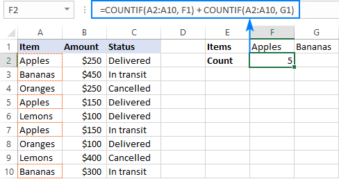
This technique works fine for a couple of criteria, but adding three or more COUNTIF functions together would make the formula too cumbersome. In this case, you’d better stick with one of the following alternatives.
Formula 2. COUNTIF with array constant
Here’s a more compact version of the SUMIF with OR conditions formula in Excel:
The formula is constructed in this way:
First, you package all the conditions in an array constant — individual items separated by commas and the array enclosed in curly braces like <«apples», «bananas’, «lemons»>.
Then, you include the array constant in the criteria argument of a normal COUNTIF formula: COUNTIF(A2:A10, <«apples»,»bananas»,»lemons»>)
Finally, warp the COUNTIF formula in the SUM function. It is necessary because COUNTIF will return 3 individual counts for «apples», «bananas» and «lemons», and you need to add those counts together.
Our complete formula goes as follows:
=SUM(COUNTIF(A2:A10,<«apples»,»bananas»,»lemons»>)) 
If you’d rather supply your criteria as range references, you’ll need to enter the formula with Ctrl + Shift + Enter to make it an array formula. For example:
Please notice the curly braces in the screenshot below — it is the most evident indication of an array formula in Excel: 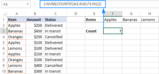
Formula 3. SUMPRODUCT
Another way to count cells with OR logic in Excel is to use the SUMPRODUCT function in this way:
To better visualize the logic, this could also be written as:
The formula tests each cell in the range against each criterion and returns TRUE if the criterion is met, FALSE otherwise. As an intermediate result, you get a few arrays of TRUE and FALSE values (the number of arrays equals the number of your criteria). Then, the array elements in the same position are added together, i.e. the first elements in all the arrays, the second elements, and so on. The addition operation converts the logical values to numbers, so you end up with one array of 1’s (one of the criteria matches) and 0’s (none of the criteria matches). Because all the criteria are tested against the same cells, there is no way any other number could appear in the resulting array — only one initial array can have TRUE in a specific position, others will have FALSE. Finally, SUMPRODUCT adds up the elements of the resulting array, and you get the desired count.
The first formula works in a similar manner, with the difference that it returns one 2-dimentional array of TRUE and FALSE values, which you multiply by 1 to convert the logical values to 1 and 0, respectively.
Applied to our sample data set, the formulas take the following shape:
=SUMPRODUCT((A2:A10=»apples») + (A2:A10=»bananas») + (A2:A10=»lemons»))
Replace the hardcoded array constant with a range reference, and you will get even a more elegant solution:
=SUMPRODUCT(1*( A2:A10=F1:H1)) 
Note. The SUMPRODUCT function is slower than COUNTIF, which is why this formula is best to be used on relatively small data sets.
Count cells with OR as well as AND logic
When working with large data sets that have multi-level and cross-level relations between elements, chances are that you will need to count cells with OR and AND conditions at a time.
As an example, let’s get a count of «apples», «bananas» and «lemons» that are «delivered». How do we do that? For starters, let’s translate our conditions into Excel’s language:
- Column A: «apples» or «bananas» or «lemons»
- Column C: «delivered»
Looking from another angle, we need to count rows with «apples and delivered» OR «bananas and delivered» OR «lemons and delivered». Put this way, the task boils down to counting cells with 3 OR conditions — exactly what we did in the previous section! The only difference is that you’ll utilize COUNTIFS instead of COUNTIF to evaluate the AND criterion within each OR condition.
Formula 1. COUNTIFS + COUNTIFS
It is the longest formula, which is the easiest to write 🙂
=COUNTIFS(A2:A10, «apples», C2:C10, «delivered») + COUNTIFS(A2:A10, «bananas», C2:C10, «delivered»)) + COUNTIFS(A2:A10, «lemons», C2:C10, «delivered»))
The screenshot below shows the same formula with cells references:
=COUNTIFS(A2:A10, K1, C2:C10, K2) + COUNTIFS(A2:A10, L1, C2:C10, K2) + COUNTIFS(A2:A10, M1,C2:C10, K2) 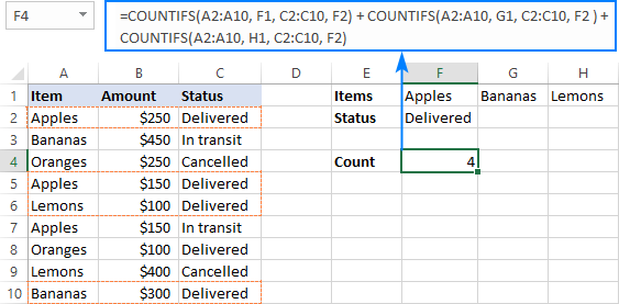
Formula 2. COUNTIFS with array constant
A more compact COUNTIFS formula with AND/OR logic can be created by packaging OR criteria in an array constant:
When using a range reference for the criteria, you need an array formula, completed by pressing Ctrl + Shift + Enter :
=SUM(COUNTIFS(A2:A10,F1:H1,C2:C10,F2)) 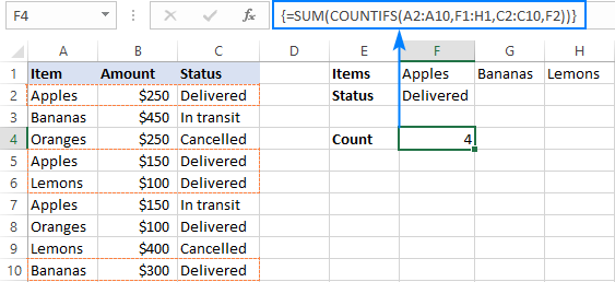
Tip. If needed, you are free to use wildcards in the criteria of any formulas discussed above. For example, to count all sorts of bananas such as «green bananas» or «goldfinger bananas» you can use this formula:
In a similar manner, you can build a formula to count cells based on other criteria types. For example, to get a count of «apples» or «bananas» or «lemons» that are «delivered» and the amount is greater than 200, add one more criteria range/criteria pair to COUNTIFS:
Or, use this array formula (entered via Ctrl + Shift + Enter ):
=SUM(COUNTIFS(A2:A10,F1:H1,C2:C10,F2, B2:B10, «>»&F3)) 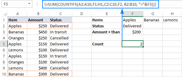
Count cells with multiple OR conditions
In the previous example, you have learned how to test one set of OR conditions. But what if you have two or more sets and you are looking to get a total of all possible OR relations?
Depending on how many conditions you need to handle, you can use either COUNTIFS with an array constant or SUMPRODUCT with ISNUMBER MATCH. The former is relatively easy to build, but it is limited to only 2 sets of OR conditions. The latter can evaluate any number of conditions (a reasonable number, of course, given Excel’s limit to 255 arguments and 8192 characters to the total formula length), but it may take some effort to grasp the formula’s logic.
Count cells with 2 sets of OR conditions
When dealing with only two sets of OR criteria, just add one more array constant to the COUNTIFS formula discussed above.
For the formula to work, one minute but critical change is needed: use a horizontal array (elements separated by commas) for one criteria set and vertical array (elements separated by semicolons) for the other. This tells Excel to «pair» or «cross-calculate» the elements in the two arrays, and return a two-dimensional array of the results.
As an example, let’s count «apples», «bananas» or «lemons» that are either «delivered» or «in transit»:
Please note the semicolon in the second array constant: 
Because Excel is a 2-dimentional program, it is not possible to construct a 3-dimentional or 4-dimentuional array, and therefore this formula only works for two sets of OR criteria. To count with more criteria, you will have to switch to a more complex SUMPRODUCT formula explained in the next example.
Count cells with multiple sets of OR conditions
To count cells with more than two sets of OR criteria, use the SUMPRODUCT function together with ISNUMBER MATCH.
For example, let’s get a count of «apples», «bananas» or «lemons» that are either «delivered» or «in transit» and are packaged in either «bag» or «tray»:
In the heart of the formula, the MATCH function checks the criteria by comparing each cell in the specified range with the corresponding array constant. If the match is found, it returns a relative position of the value if the array, N/A otherwise. ISNUMBER converts these values to TRUE and FALSE, which equate to 1 and 0, respectively. SUMPRODUCT takes it from there, and multiplies the arrays’ elements. Because multiplying by zero gives zero, only the cells that have 1 in all the arrays survive and get summed.
Th screenshot below shows the result: 
This is how you use the COUNTIF and COUNTIFS functions in Excel to count cells with multiple AND as well as OR conditions. To have a closer look at the formulas discussed in this tutorial, you are welcome to download our sample workbook below. I thank you for reading and hope to see you on our blog next week!
Practice workbook
You may also be interested in
Table of contents
Let’s say I have 2 columns Column A — 1-20 and Column B — 31 — 50. How can I count the unique entries when column A is > 10 or Column B is > 40. Kindly help.
Hello!
If I understand your task correctly, the following tutorial should help: Count unique values with criteria.
I am creating schedules for our staff. Using below data and trying to count the actual working employees total and ignore employees those are on training and days off. I am using this formula but its not working . Please help me
=SUMIF($D$6:$D$14,»TRAINING»,F6:F14) + SUMIF(F6:F14,»D/O»,F6:F14)
AM Leads 05:45 — 14:15
D E F G H
LEADS EMPL # Sun Mon Tue Wed Thu Fri Sat
1 TRAINING D/O D/O 05:45 — 14:15 05:45 — 14:15 05:45 — 14:15 05:45 — 14:15 05:45 — 14:15
2 ANNY 05:45 — 14:15 05:45 — 14:15 D/O D/O 05:45 — 14:15 05:45 — 14:15 05:45 — 14:15
3 PERRI 05:45 — 14:15 05:45 — 14:15 05:45 — 14:15 05:45 — 14:15 D/O D/O 05:45 — 14:15
4 JAM D/O 05:45 — 14:15 05:45 — 14:15 05:45 — 14:15 05:45 — 14:15 05:45 — 14:15 D/O
5 KLM 05:45 — 14:15 D/O D/O 05:45 — 14:15 05:45 — 14:15 05:45 — 14:15 05:45 — 14:15
6 BOBBY 05:45 — 14:15 05:45 — 14:15 05:45 — 14:15 D/O D/O 05:45 — 14:15 05:45 — 14:15
7 TRAINING 05:45 — 14:15 05:45 — 14:15 05:45 — 14:15 05:45 — 14:15 05:45 — 14:15 D/O D/O
8 TRAINING D/O D/O 05:45 — 14:15 05:45 — 14:15 05:45 — 14:15 05:45 — 14:15 05:45 — 14:15
9 TRAINING 05:45 — 14:15 05:45 — 14:15 D/O D/O 05:45 — 14:15 05:45 — 14:15 05:45 — 14:15
Daily Total 6 6 6 6 7 7 7
Actual Daily 4 4 0 0 0 0 0
Variance +(-) 2
Hi!
Use the COUNTIF function instead of the SUMIF function as described in the article above.
Hi sir,, thanks so much for yo class it’s very interesting I’ve added something new..
Can you let me know if there is an excell formal that can colour the cell with a certain commands??
Hi!
I don’t really understand your question, but maybe you need to use conditional formatting.
I mean that,, is there a formula that can help me to make a cell coloured??
Hi!
Take a look at the article I recommended to you earlier. This guide may also be helpful: Excel conditional formatting formulas based on another cell.
Hi
My current issue is i have to sheets lets say
Sheet1 is where the formula is so
Countif(sheet2A:A;$C$3) this formula will be in cell C5 and the C6,C7, C8
What i need is to move the auto fill series to move ranges on sheet2 to be filled as the formula on C6 to query B:B, C7 to query C:C and so on
Can you help me with that please
Hi!
Copying the formula down may change the row numbers, but not the column numbers. Autofill is not working the way you want.
You can dynamically change cell addresses in formulas using the INDIRECT function.
What do I do if I need to do count cells with multiple sets of OR conditions, but one of or conditions is not match, but rather a countif (ie >0)? Thanks!
Hi!
Have you tried the ways described in this blog post? If they don’t work for you, then please describe your task in detail, I’ll try to suggest a solution.
Hi, I’m trying to assemble multiple AND/OR logic. The first group I can solve with SUM(COUNTIFS, but getting stuck after the OR logic
Count cells if:
column F is one of: «*Scope*»,»*Component*»,»*Vendor*» AND column E = A2 (let’s call this group1)
OR
column F = «*Decommission*» AND column I «*Production*» AND column E = A2 (let’s call this group2)
Final result should be total cell count of group1 + group2
(wildcards intentional)
Thank you
note in the second group column I doesn’t equal «*Production*» — looks like my symbols were removed
Hi!
Have you tried the ways described in this blog post? It covers your case completely.
Here is an example formula
I have excel sheet for result analysis range H7:ET600. I have to count «AB» from some columns only. I can’t select range because columns other than these one also have «AB» entry. how I can count it?
Hi!
If I understand your task correctly, the example following formula should work for you:
Specify each column individually.
How to count the occurrence of each number (range from 1 to 14) in a cell with a number pattern 1/12/5/1/13/10 or 10/11/9 or 8/5 ?
Hello!
Split this text into cells using this guide: How to split cells in Excel: Text to Columns, Flash Fill and formulas. Then count the number of times the number appears in the range using the COUNTIF function.
Good day
I’m trying to automate a count on a per class basis and a age.
my current formula is this:
This is returning a value of 0
but if I do the counts separately I get the correct values. so «count class1», gives 39 and count (the different years) gives a value of 151 (as its searching the whole data set, but I only need it to count for class1 (Which is actually from A3 to L41) but I want to future proof for if I add or remove from the set
So the count cant be 0
I think i may have figured it out.
=SUM(COUNTIFS(‘PC Spec CPT’!$B$3:$B$171, «*CLASS1*»,’PC Spec CPT’!$J$3:$J$171,<«5 years»,»6 years»,»7 years»,»8 years»,»9 years»,»10 years»>))
Appears to give the correct result. I just needed to isolate the columns for the 2 criteria instead of doing the whole data set
Hi!
The COUNTIFS formula counts the rows where all the criteria are met once. But at the same time, it cannot work with a range ($A$1:$L$171), but only with a data column ($A$1:$A$171).
Awesome! Thanks a lot for all clarifications in here!
I have a spreadsheet with data collected from an electronically completed survey. Some of the columns are free text entry from the form. I want to summarise the submissions and categorise according to job role. However, there are a huge number of terms used for example for doctors. «registrar», «SHO», «consultant» «consultant anaesthetist», «anaesthetist», «FY2», «clinical fellow» etc. I am trying to use SUM and COUNTIFS to give me the number of forms that were submitted for a group of staff in one month. However, I am getting entries double counted as if the free text includes «consultant anaesthetist» then it is being counted twice as I want to ensure that entries that have only described the doctor as a consultant or anaesthetist are counted.
This is my formula I have named ranges Date and Recipient, H5 and I5 are cell references to specific dates.
Hello!
To avoid double counting, in a separate column, write something like this SEARCH formula with all the words you need. Then use that column to count in the COUNTIFS formula.
Good morning! You all are so incredibly helpful, I just hope I can describe my issue well enough for you to understand! I have a table that looks like this:
Virtual Virtual Virtual
Onsite Onsite
OTT OTT
Jon X X X
Dan X X X
Rob X X X
Tim X X X
I need to count the number of times each person is either Onsite or OTT. The results I should get are:
Jon 2
Dan 1
Rob 0
Tim 3
However, when I try to use normal COUNTIFS it counts Jon and Tim twice because column C has both Onsite AND OTT. I need it to count Onsite OR OTT. I tried to use the OR logic you outlined. =SUM(COUNTIFS($B$1:$G$3,<«Onsite»,»OTT»>,B4:G4,»X»)) but that doesn’t work with multiple rows. How can I get this to calculate correctly? I feel like I’m so close.
Okay, so multiple spaces get stripped out. Let’s try with dots.
. Virtual. Virtual. Virtual
. Onsite. Onsite
. OTT. OTT
Jon. X. X. X
Dan. X. X. X
Rob. X. X. X
Tim. X. X. X
I am working on a spreadsheet with Start Date, Resolve Date, and Status. I want to look at the amount of work being done in the current month. For example, if I’d like to look at the number of things completed in August, I could count everything initiated in August that has a complete status PLUS everything resolved in August with a complete status. BUT, the problem is that some things can be initiated in August and Resolved in August, which would cause the same issue to be double counted.
My current formula for counting total complete based on start date is
=COUNTIFS(StartDate,»>=»&EOMONTH(TODAY(),-1)+1,StartDate,»=»&EOMONTH(TODAY(),-1)+1,Resolved,» Reply
I typed in two formulas, but it looks like it somehow got combined into two?? They should be as follows:
Based on start date:
=COUNTIFS(StartDate,»>=»&EOMONTH(TODAY(),-1)+1,StartDate,»=»&EOMONTH(TODAY(),-1)+1,Resolved,» Reply
I don’t know why this keeps happening. There are two formulas that I’m typing in, with a new paragraph between them. My paragraph keeps getting deleted and the formulas partially combined.
Hello!
I can’t check the formula that contains unique references to your workbook worksheets. Count the records that meet the first condition, add the records that meet the second condition, and subtract the records that meet both conditions.
=COUNTIFS(StartDate,”>= ”&EOMONTH(TODAY(),-1)+1,Status,»Completed») + COUNTIFS(Resolved,” =”&EOMONTH(TODAY(),-1)+1, Resolved,” Reply
I am trying to create a column that will provide me a subset of orders that need to be reconciled between two ERP systems. However, there are three different types of ways that one system will recognize an order.
I am hoping that this column will catch IF it exists in one system under one reference, but right now there are cases where an order can be recognized by all three references, just depends on user input.
Trying to acheive a formula that will count Order Ref 1 OR Order Ref 2 or Order Ref 3. If the system recognizes it as Order Ref 1 / Order Ref 2 I only want it to count once towards the total subset.
Current formula: =COUNTIF(‘TMS DATA’!A:A, Table2[[#All],[Order ‘#]])+COUNTIF(‘TMS DATA’!A:A,Table2[[#All],[Shipment’#]])+COUNTIF(‘TMS DATA’!A:A,Table2[[#All],[Order ID]])
Can you help me with the OR part that I am missing? I feel like I am just counting them all.
Hi!
It is very difficult to understand a formula that contains unique references to your workbook worksheets. Unfortunately, without seeing your data it is difficult to give you any advice. Please provide me with an example of the source data and the expected result.
Can anyone help with the formula?
I have 10 drivers and 10 vehicles, Each day wages of driving individual vehicle is different. I.e Vehicle A wages 500, vehicle B wages 1000 and Vehicle C Wages 1500. Now Driver A had drove those vehicles in term of 15 days. How would I calculate this with the formula.
Hello and thank you for you dedication to helping people!
I believe there is an issue with the AND/OR logic part of the article in that the formula generates «false positives» which must be subtracted to get a correct answer.
LIST A LIST B LIST C LIST D
TRUE TRUE TRUE TRUE
TRUE TRUE TRUE FALSE
TRUE TRUE FALSE TRUE
TRUE TRUE FALSE FALSE
TRUE TRUE TRUE TRUE
TRUE TRUE TRUE FALSE
TRUE FALSE FALSE TRUE
TRUE FALSE FALSE FALSE
TRUE FALSE TRUE TRUE
TRUE FALSE TRUE FALSE
TRUE FALSE FALSE TRUE
TRUE FALSE FALSE FALSE
For instance, if (A and B) or C or D are true in the above data the result should be 5 (not 7) as below:
Here’s the rub. If I have additional columns (not shown and also not actual data) and need to find (A and B) or C or D or E or F or G or H or I or J or K or L in a list of 100,000 items (peak season), is an elegant solution possible?
Thanks and I do appreciate your work!
Hi!
Your formula returns 5. But if I understood your conditions correctly, the result should be 3.
If I understand your task correctly, the following formula should work for you:
I hope I answered your question. If something is still unclear, please feel free to ask.
Thank you for the prompt response. Unfortunately I did not clearly state the full nature of the problem.
Data is not «true» or «false» but could be text, currency, value, date, blank, etc.
Each line is counted only once based on conditions further explained as follows:
List A and List B must both be «true» for a line to be counted.
Lists E through L must have at least one condition «true» for a line to be counted.
Each line may only be counted as one instance.
So lines 1, 2, 3, 5, 6 should be the only lines counted for a total of 5 lines meeting the conditions.
Helper columns discouraged because of the size of the data.
I perceive this as Wizardry at this point.
Hi!
If I understand your task correctly, try the following formula:
Sir, that is a brilliant and imaginative solution! This is a truly remarkable method for implementing complex AND/OR conditions in Excel. Thank you and may the formulas be always in your favor.
Hello. The «count cells with multiple sets of OR conditions» formula described above was extremely helpful for me. Thank you!
Let’s say there’s a «Date_Shipped» column in D:D.
Hello!
If you write dates in column B, then you can compare them with the desired date using the DATE function.
Thank you! I was not familiar with the double minus (—). This is exactly what I needed and the formula works like a charm. CHEERS!
I have a worksheet that I am working for work. Basically, I would like to count how many people visit the park (column A) in both year 2020 and 2021(column B). Column B only shows either 2020 or 2021.
This formula: =SUM(COUNTIFS(Table2[List YR], <«2020″,»2021»>, Table2[COUNTY], A2))
— provides number of people that visit on 2020 and number of people that visit on 2021, not the number of people that visit both year.
This formula: =COUNTIFS(SPEC!A:A,A2,SPEC!B:B,2020,SPEC!B:B,2021)
— provides 0
Hello!
Add column C to the table with the formula
Count the number of people using COUNTIFS:
I hope my advice will help you solve your task.
If a student gets mark less than 16 or his average be less than 50 he must be in group D. Please write a formula for it
Hi!
Please check out this article to learn how to write an IF OR statement in Excel to check for various «this OR that» conditions.
Hello!
My husband is trying to create a spreadsheet for work and cannot seem to find a formula that works.
He is trying to use the COUNTIFS function to count all cells in a range that are within separate number ranges.
He needs the cells to be counted once if they are below 517, or between 525 and 896, or above 905. Every formula we have tried has not worked. It either does not count the cells, or counts them more than once.
This is an example of one of the formulas we have tried:
I know this is not right, but I have scoured the internet but have not found a solution.
Hello!
You can find the examples and detailed instructions here: Count cells with OR conditions in Excel.
I hope I answered your question. If something is still unclear, please feel free to ask.
Hey, can you help me with a google sheet formula?
It seems that Google Sheet can only count the total number of «Barry» but NOT BOTH «Barry» and «Maya», is there a way to fix this?
I believe you will find these instructions for Google Sheers helpful:
Count in Google Sheets with multiple criteria — OR logic
=SUM(COUNTIF(‘Signed Case’!C:C,<«Barry»,»Maya»>)) — Wrong Formula
=SUM(COUNTIFS(‘Signed Case’!C:C,<«Barry»,»Maya»>)) -than press Ctrl+shift+Enter
I have been trying to count the number of LGBTQ+ from an organization. However, the code
does not seem to work. Here is a sample of my work. I hope you can visualize it.
Note: COUNTIFS or COUNTIF, still does not work. It does not count the «Bi»
I am trying to count Yes and No in 1 cell but from multiple columns and then create a score in another column. So if I got 3 «yes» and 1 «no» the score would be 3. This what I got:
=SUM(COUNTIF(U3,N3,X3,<«Yes»,1>)(U3,N3,X3,<«No»,0>))
But it did occur to me that I don’t need to count the «No» so could I shorten it thus?
=SUM(COUNTIF(U3,N3,X3,<«Yes»,1>)
I’m getting errors saying I’m entering too many arguments and it doesn’t work. Help!
Trying to find a solution for nested conditions with no success so far. Please see below:
Spreadsheet is looking to see if a range of cells (D:32:D35) is answered «Yes», If 1-2 cells in this range are answered «Yes», then cell L:31 will be assigned a value of .5. However if greater than 2 cells in the range answer «Yes». then L:31 will need to be 1.
Any tips? Thank you!
Hi!
If I got you right, the formula below will help you with your task:
Since, after multiple attempts, I can’t seem to get my formula to show correctly, can I email it? It shows fine, until I hit Send and then half of it is missing.
We apologize for this nasty behavior. Our blog engine often mangles formulas containing «less than» and «greater than» operators, and we can do nothing about it. You can email your formula to support@ablebits.com Att: Alexander Trifuntov
Again, our apologies for the inconvenience.
Thank you for your emailed response, which worked.
SUMPRODUCT(—(AND(‘Source Sheet’!$D:D>=A3,’Source Sheet’!$D:D0,1,0))
I don’t understand why the formulae are being truncated.
Breaking it up, will see if that works
=SUMPRODUCT(—(AND(‘Source Sheet’!$D:D>=A3,’Source Sheet’!$D:D0,1,0))
I want to count, only once, those values that match ONE of a range of three criteria. Column A contains dates and multiple rows can have the same date. Columns B, C or D contain only «Y» or «N». I want to count, for each date, only those rows where a «Y» is in any one of B, C or D. If there is an N in all three, it is not counted. For example:
01/01/2021 Y N N
01/01/2021 N N Y
01/01/2021 N N N
01/01/2021 Y Y Y
02/01/2021 Y Y Y
The count against 01/01/2021 should return 3 above, because there is at least one Y in cols B, C or D on three of the four rows that match that date (where there is more than one, it should only be counted once).
No variation of SUMPRODUCT, COUNTIFS etc I have come up with gives me the right number. Can you help please?
Hello!
Please check the formula below, it should work for you:
I hope this will help
It does for individual dates, thank you. I also have a monthly summary sheet. In this one, months (eg Jan-21, Feb 21 etc are in column A of the summary sheet, to be checked against individual dates on column D of the source worksheet and the data to be checked for a single Y are in columns E to G of the source worksheet. I have attempted to adapt the formula you gave but this returns a VALUE error. I am guessing it is a simple missed comma or bracket, or is it the AND throwing it out?
=SUMPRODUCT(—(AND(‘Source Sheet’!$D:D>=A3,’Source Sheet’!$D:D0,1,0))
This is attempting to count, for all dates between 1st and last date of the month in column A of the target sheet, where there is a Y on each row in any one of columns E to G in the source sheet,
For example, if A3 on the target sheet were Mar-21, it would retrieve all values where the date is greater than or equal to 1st March 2021 and less than or equal to 31st March 2021 and, for the rows between those dates in the source sheet, count how many of those rows have at least one Y between cells E and G and output that number to the cell containing the above formula in the target sheet. Note, I have ruled out using just month numbers as the source sheet contains more than one year of dates.
Some of the formula was missing in my last comment. Trying again
=SUMPRODUCT(—(AND(‘Source Sheet’!$D:D>=A3,’Source Sheet’!$D:D0,1,0))
I am creating an spreadsheet for our Oncology dept which has the following sheets say 3 March, 4 March, 5 March etc and then a summary page. Each days sheet contains the Patient ID as well as what type, namely chemo, New File, Others etc. In the summary page I need to show a summary count with each of the category (Chemo,New Fileetc.) under a day column like this
05 March 2021 06 March 2021 07 March 2021
Morning Session — New File 1 #VALUE!
Morning Session — Chemo 2
Morning Session — Old 1
Morning Session — Others 0
***** 4
The COUNTIFS formula works when I dont have to evaluate the date to the current date which I have given as a heading and then in a cell in the days (6th March sheet). That throws an error. This is the formula I have used
=COUNTIFS(‘6th March’!E5:E1335,»Chemo», ‘,Summary!C2,’6th March’!C2)
Where the second criteria is the date I am trying to collate.
Any help will be much appreciated.
Thank you in advance.
Hello!
Unfortunately, without seeing your data it is impossible to give you advice.
I’m sorry, it is not very clear what result you want to get. Could you please describe your task in more detail and send us a small sample workbook with the source data and expected result to support@ablebits.com? Please shorten your tables to 10-20 rows/columns and include the link to your blog comment.
We’ll look into your task and try to help.
I am currently working on a formula to track 3 different types of orders and their status. In the workbook I have the order type as well as the due date and completion date in separate columns. I also created 2 columns to calculate IF statements to determine if 1) the order is «overdue» (completion date>due date) and 2) if the completion date is «blank» to mark it as outstanding. Currently I have the formula set to count any of the specific order type that is marked as overdue or as outstanding (Formula:=COUNTIFS(‘Due Dates’!$A:$A, T18,’Due Dates’!I:I, «OVERDUE»)+COUNTIFS(‘Due Dates’!$A:$A, T18,’Due Dates’!J:J, «OUTSTANDING»); however, I want to narrow it down further so that only pulls the overdue+outstanding count from a specific due date instead of from everything. What function should I use to go about this? Thank you!
Hello!
If I understand your problem correctly, one more condition needs to be added to each of the COUNTIFS formulas. Like that:
=COUNTIFS(‘Due Dates’!$A:$A, T18,’Due Dates’!I:I, «OVERDUE»,’Due Dates’!B:B,»>»&T19 )+COUNTIFS(‘Due Dates’!$A:$A, T18,’Due Dates’!J:J, «OUTSTANDING»,’Due Dates’!B:B,»>»&T19)
where T19 is the date to count.
Hope this is what you need.
Help me with the count function for a number and a text on the same range. For example, I want to count cells based on attendance, if it is Y, it should be considered, if I update as 1 or 30, it should also be counted for all the data
Hi,
If I understand your task correctly, the following formula should work for you:
I hope this will help
Need help. I need to an item in a separate excel spreadsheet to be counted based on two conditions in a worksheet. I need it to count the item once if the Part No of the item (for example is 01667-1″ and the order number column is populated with an all numerical number (for examples » 1234″ or #1556″). The numerical number is unique except for the first number so I tried using a wild card. Oh and one more thing the numerical column (G:G) may have blanks. The count is populated into a different worksheet.
I wrote this one but its not working. My result says 0 when I know I currently have 18 items like this.
=COUNTIFS(‘ Fruit Config Flow’!$C:$C,»01667-1″,’ ACCG Config Flow’!$G:$G,»1*»)
Hello!
The COUNTIFS function uses only range references as criteria_range. Therefore, you cannot use COUNTIFS in your case.
Try this array formula:
This is an array formula and it needs to be entered via Ctrl + Shift + Enter, not just Enter.
$K$1 is «01667-1»
I hope I answered your question. If something is still unclear, please feel free to ask.
Hello, I am trying to write a function that will count employees with either blank termination dates or termination dates after 1/1/20. The other criteria is all of these employees have to be from NYC. The function I have is =SUM(COUNTIFS(Q:Q, <«», «>1/1/2020″>, G:G, «New York»)). It only seems to be counting the blanks and not adding term dates post 1/1/20 to the total count. Any advice for resolving would be very appreciated!
Hello!
If I understand your task correctly, the following formula should work for you:
=COUNTIFS(Q:Q, «», G:G, «New York»)+COUNTIFS(Q:Q,»>1/1/20″, G:G, «New York»)
You can learn more about count cells with OR conditions in Excel in this article on our blog.
I want to count the number of cells that have a number in them, not if it is blank.
Hello!
Here is the article that may be helpful to you: COUNTIF in Excel — count if not blank.
I hope it’ll be helpful.
Hello! GREAT ARTICLE, but as a German Excel user there remains a crucial question:
«Count cells with 2 sets of OR conditions»
«Please note the semicolon in the second array constant»
Well, semicolon is the standard in Germany for the comma (as in probably all European countries). Can somebody tell me what would be the equivalent for that semicolon then in Germany? Thanks a lot in advance.
Thanks
David
by the way it is not comma
I just got it! I downloaded one of the files on this site where the formula I meant is included — and my German Excel converted it automatically to German enterings. It would be «» in Europe 🙂
Could you help me with a formula — I have a pack slip for warehousing and I’m trying to sum the total of packages that have either «1» OR «13» items (cell range D10:D20) AND are being shipped via any of the following carriers «GSO», «VINGO», or «UPS» which are listed in cell range C10:C20. I currently have the formula as =SUM(COUNTIFS(C10:C20, <«GSO», «UPS», «VINGO»>, D10:D20, <«=1»; «=13»>)) but it’sa not returning the correct results. Help?
Hello!
The formula below will do the trick for you:
=SUM(COUNTIFS(C10:C20,<«UPS»,»GSO»>,D10:D20,<«1″,»13»>))
if your numbers are written as text
I have the data I want to add together in column I. I only want to count the data in column I for specific criteria/names in column B.
I am struggling putting together the formula to achieve this sum for column I based on criteria in column B.
Hi I am trying to do the following COUNT formula:
If cells J20:J44 are greater than 0 but less than 50
Thank you in advance
Hello!
You have 2 conditions for counting. So use the COUNTIFS function
I couldn’t get the neater «OR» countifs function to work (Formula 2: countifs with array constant). The longer formula 1 (Countif + Countif) does work, but isn’t as tidy.
Here is your example:
=SUM(COUNTIFS(A2:A10, <«apples»,»bananas»,»lemons»>, C2:C10, «delivered»))
My version is attempting to count the number of people who took a certain course in 2019 OR 2020 (adding the number of delegates from 2019 and 2020 together for a specific course).
=sum(COUNTIFS(‘Form responses 1’!B:B,<«2020″,»2019»>,’Form responses 1′!D:D,»Course X»)) where column B is the year column, column D is course name (redacted for the purposes of this post)
However this formula will only return numbers from 2020. Swap the years around, it only returns numbers from 2019. I would like them added together.
Any ideas what I’m doing wrong?
Hello!
Unfortunately, without seeing your data it hard to give you advice.
I can assume that in your table ′Form responses 1′!B:B,the year is written not as text, but as a number.
Therefore, do not use quotation marks — <2020,2019>.
I recommend using the SUMPRODUCT function for counting. Read more here
I hope it’ll be helpful.
Hello. Can you please help me figure out how to count how many times a value occurs between two date columns?
I’m trying to count how many, let say «installs,» occur per week with the start at end date columns.
There is more than one row with start dates and end dates that overlap and I’m trying to break it down by how many are overlapping in each week.
Column B & C are the start and end of the install. E and F are just part of my model.
For example, someone may have 44 installs per year, but how many are occurring each week at the same time.
I’m trying to show how many installs occur/overlap to the right of columns E and F via column G.
Link to the spreadsheet: https://docs.google.com/spreadsheets/d/1krnLiVUTfXWIWh0PTVXqK9Zpy5lNegYHoUWGMTruI88/edit#gid=997917131
Here are some formulas I have tried:
1. =SUMIFS($H$3:$H$44,$G$3:$G$44, >=K3&)+SUMIFS($H$3:$H$44,$G$3:$G$44, «&K2,$A$2:$A$217,$H$2:$H$217,»=K3″>,0))*ISNUMBER(MATCH($H$3:$H$44, <» Reply
Hi there. I am struggling to write a formula to count all data that meets the following criteria: Male (column IN, data criteria is «1»), and age 25-64 (column IO, data criteria is «2, 3, 4, 5, 6, 7, 8, or 9»), and college educated (column IS, data criteria is «5 or 6»), and employed full-time (column IT, data criteria is «1»), and HHI of $50-75k (column IV, data criteria is «5»), and white (column IX, data criteria is «3»), and in the south (column JI, data criteria is «2»), and in data wave 1 (column B, data criteria is «1).
Separately, next I’ll need to add another criteria layer to the above. Answered Q1 as «Not very concerned» (column C, data criteria is «3»). But I’ll need this count value turned into a % of the total count (above).
Can you please help?
Hello Alexis!
I hope you have studied the recommendations in the above tutorial. Read «COUNTIF-multiple-criteria-AND-logic». Please let me know in more detail what you were trying to find, what formula you used and what problem or error occurred. In that case I will try to help you.
Hi Alexander. Yes I have studied the above.
I first need to count the # of people who fit this criteria: In data wave 1 (column B, data criteria is «1»), and Male (column IN, data criteria is «1»), and age 25-64 (column IO, data criteria is «2, 3, 4, 5, 6, 7, 8, OR 9»), and college educated (column IS, data criteria is «5 OR 6»), and employed full-time (column IT, data criteria is «1»), and HHI of $50-75k (column IV, data criteria is «5»), and white (column IX, data criteria is «3»), and in the south (column JI, data criteria is «2»).
This returns #VALUE! error: =SUM(COUNTIFS(CSVData4241!B:B,1,CSVData4241!IN:IN,1,CSVData4241!IO:IO,<«>=2″;
=5″;»=2″,»=5″,» Reply
Looks like my example formulas got cut off. Please see below:
This returns #VALUE! error: =SUM(COUNTIFS(CSVData4241!B:B,1,CSVData4241!IN:IN,1,CSVData4241!IO:IO,<«>=2″;
=5″;»=2″,»=5″,» Reply
Hello Alexis!
If I got you right, the formula below will help you with your task:
=SUM(COUNTIFS(B2:B8,1,IN2:IN8,1,IO2:IO8,<2,3,4,5,6,7,8,9>, IS2:IS8,<5,6>,IT2:IT8,1, HHI2:HHI8,5,IX2:IX8,3,JI2:JI8,2))
Change the cell addresses to suit your task. I hope you understand that you can use an array of values for several conditions.
Can you help me with one formula? I’ve been struggling for a while to get it right.
I am trying to capture (COUNTIFS) a certain employee has either not delivered a report in time (past its due date) or if he has delivered it, but past its due date. In my current raw data i have the Employee Name, Due date, the Delivery date (which can be blank while its not yet delivered, or filled if delivered) the name of the employee & the status of a report (its «draft» if its still not delivered; its «Final» or «Provisional» if it has been delivered).
I’d highly appreciate if you could help me out. It’s been bugging me for some time!
Thanks in advance!
Hello Aline!
If you want to have the report delivery status for each employee (in Column H, for example), please use this formula:
=IF(C2<>«»,IF(B2>C2,»OK»,»Past due date»), «Not delivered»)
There is a due date in Column B and a delivery date (or nothing) in Column C here.
If it is necessary to count how many reports are overdue or not submitted, please use this formula:
If you still have questions, please ask.
I have a spreadsheet that has pressure in one column from row 4 to row 54435. I have multiple pumps (the pumps have either a 0 for off or a 1 for running in each row) Each pump being in a separate column with rows 4 through row 54435. What I need to do is count a specific pressure rating range (PSI between equal to or greater than 85psi but less than 86psi). But the catch is that I want to count the pressure only once with any of the pumps running. So for example if I have pump 5 running OR pump 6 or any of the other pumps are running AND the pressure is between 85 and 86psi, I want to count it once. I would like to do this for multiple pressure settings. I have used Countif(PSIRange,»>»&»=»85, PSIRANGE,» Reply
Hello Ray!
If I understand your task correctly, maybe the following formula should work for you:
=SUMPRODUCT(— (PSIRANGE>=85), — (PSIRANGE Reply
Hi, I am wondering if someone can help me figure our how to combine COUNTIFS formulas. For example, I need to present this more efficiently:
=COUNTIFS(VAR1,”Yes”,VAR2,»2016″,VAR3,»Q1″,VAR4,PH,VAR5,»Pres») +
COUNTIFS(VAR1,”Yes”,VAR2,»2016″,VAR3,»Q1″,VAR4,»Both», VAR5,»Pres») +
COUNTIFS(VAR1,”Yes”,VAR2,»2016″,VAR3,»Q1″, VAR6,PH, VAR5,»Pres») +
COUNTIFS(VAR1,”Yes”,VAR2,»2016″,VAR3,»Q1″, VAR6,»Both», VAR5,»Pres»)
So I need counts if VAR1 =Yes; VAR2 = 2016; VAR3=Q1; VAR5=Pres; AND VAR4= PH or Both; AND VAR6=PH or Both. I think the way I have it does the job, but I’m sure there is a more concise way to write the formula as it may get very long as I add criteria to it.
Hello E Safi!
If I understand your task correctly, the following formula should work for you:
I hope this will help, otherwise please do not hesitate to contact me anytime.
I am having the same problem like «E Safi» but rather than using direct literal text. I need to use wild card as it is group in a single cell. below is a working formula but the problem is it counts the cell twice if it contains both the word «PH» and «Both». is there anyways that it will be only counted once?
=SUMPRODUCT(—(A1:A4=»Yes»),—(B1:B4=2016),—(C1:C4=»Q1″),((D1:D4=»PH»)+(D1:D4=»Both»)),—(E1:E4=»Pres»),(ISNUMBER(SEARCH(«*PH*»,F1:F4)+ISNUMBER(SEARCH(«*Both*»,F1:F4)))))
Hello Russel!
If I understand your task correctly, the following formula should work for you:
=SUMPRODUCT(—(A1:A4=»Yes»),—(B1:B4=2016), —(C1:C4=»Q1″),((D1:D4=»PH»)+(D1:D4=»Both»)), —(E1:E4=»Pres»), (ISNUMBER(SEARCH(«*PH*»,F1:F4))+ISNUMBER(SEARCH(«*Both*»,F1:F4))))
I hope it’ll be helpful.
I have rows of numbers (thousands of them) and dozens of columns with numbers in them. Some of the numbers are formatted as dates, some are formatted as time and some are formatted as Number/Fixed/2. All the numbers in the columns are the same format. The database is large and has a lot of blank cells because there is no data available.
I would like a COUNTIF formula which would tell me how many (for example) non-blank cells in the row are formatted for Number/Fixed/2.
I’m trying to count «Agree» and «Strongly Agree» in columns h:k, but only if column D=»Tony»
I already tried this formula =SUM(COUNTIFS(PreWorksheet!H:K, <«Agree»,»Strongly Agree»>, PreWorksheet!D:D, «Tony»)) and it’s not working. I keep getting the #VALUE error.
Any help is appreciated.
TIA
Can you help me with formula?
Assuming the range A1:A20, I need to count the number of cells that:
1- Not Blank
2- Does not equal «Red» or «Blue» or «Green»
3- Does not contain Numbers
No matter what I try, I still get the wrong count.
Can anyone help me please?
Thanks!
Hello, thank you for your detailed explanations of the functions. I am currently trying to count using count if plus OR and none of the above mentioned seemed to be working. Im trying to count if column A has Yes and if either column B or C are blank, unfortunately right now it does a double count if both B and C are blank. I would be grateful for your help. Unfortunately there is no minimum value and it has to be blank
Hello, i am working with work orders. Specifically the comments technicians write about the work orders and i am counting specific words used like «hot», «cold», «temperature», etc.
example:
STORE COMMENT
1 Unit is too hot
2 Unit moves from cold to hot
3 Temperature not holding
4 Temperature is too cold
5 Unit is too cold
I am using «* *» in my countif to search within text, like «*hot*» would come back as «2». my question is, how can i do a countif, countifs, or sum to count «*cold*» + «*hot*» + «*temperature*» without double counting comments that contain two of those key words. For example, with the above data, i want the count to be «5» but if i follow the above instructions it would count store 2 and store 4 twice, giving me a total of «7». any thoughts?
I was hoping you could help me with a table i’m trying to create. I want to «reverse» the countifs formula i’ve got to get the results it has counted (as if it was a pivot table).
My formula looks like this: =SUM(COUNTIFS(‘worksheet1′!$B:$B,»Criteria1″,’worksheet2’!$W:$W, <«criteria2″,»criteria3»>))
As you’ll see this is multiple criteria (criteria1 AND (criteria 2 OR 3)).
What I then need to do is something like a complex vlookup to find the rows that the formula has counted and then pick specific cells to return.
Imagine my table having 25 columns. My criteria are in columns 2 (B) and 23 (W) and I want a formula that will help me return values from column 1 (A) for any row counted with the countif formula mentioned earlier.
Hope that makes sense.
Thanks so much for this tutorial, it was hugely helpful and very easy to follow!
I found that I didn’t need SUM for the leave chart I created counting letters in a column. I just used:
And it gave me the correct summed number. Worked in 2016 and 2010.
Nope, definitely need SUM!
did a repost since part of my post was not reflected above.
A very good post and may have a solution for me as well. I’ve tried myself but could not get through.
So, I have 2 types of data in my table:
— some columns use only text and
— other columns use dates or text.
I need «COUNTIFS» with «OR» functionality for Date fields and WILDSCARDS («>=» or » =» or » Reply
why not working countif(range,and()) ?
I’ve been trying to formulate my sheet to count between numbers.
For example I have a host of different variables from 1.50 to around 100 and I wish to count them in sections, to explain further I want to count YES, NO VOID between 1.50 — 1.66 / 1.72 — 1.80 / 1.83 — 2.00 / 2.10 — 3.50 / 4.00 — 6.
I’ve tried to replicate these above formulas but most only count words and not numbers between ranges.
Can anyone provide any help?
Thank you
I know this is a long shot however, I am currently having issues with creating a formula to read the following.
Name score1 score2 score3
smith 58 55 61
in the example above I need to create a formula that will count the number of cells w/ a score below 60. however, this issue I am having is I need the formula to only count this as a multiple failed event by one person and not read the formula as two cells Reply
Some examples of formula I have been using are
=countif(E198:E262,» Reply
And if a certain person has one or more scores under 60, what do you want to return? Simply 1, or something else?
Could you please help me to create a formula for the scenario mentioned below.
Column A contains various product names like Apple, Cherry, Banana, Grapes etc every product has more than 5 count in Column A
And Column B has only words like Bought and Sold for every other products
I want to create the formula to every product either of these
1. How many sold and bought for grapes, banana, apples etc
2. Which trade is greater is it Bought or Sold for every products.
I may be under the wrong impression but, technically, all of your suggested solutions seem to work only as an AND fuction. That being said, your suggestions don’t work well with my need of the real OR function in countif formula. Allow me to explain my problem.
I have a list of phrases in column A, position numbers in column B and another position numbers in column C. Now, I need to count all the phrases in column A that have the position Reply
A simple solution that comes to mind is to create a helper column (you can hide it or move to the end of the worksheet) and pull the smaller of the 2 values there: =MIN(B2:C2)
And then, you use COUNTIF on the helper column, e.g.=COUNTIF(D2:D100,» Reply
Thanks
many many love to you. This trick was really awesome.
Can you help me with a formula?
I have some student test scores and I’d like to create a formula that tells me how many students in each class got above the year average, and how many got below. But, there are some absent students, so I’d like to only count the scores above 0.
This is my current formula for above average scorers in class 1: =COUNTIF(AD7:AD45,»>»&$AD$287)
This is my current formula for below average scorers in class 1:
=COUNTIF(AD7:AD45,» =AVERAGEIF(AD7:AD285,»0″) ]*
These formulas work, but the below average formula also includes scores for students who were absent and didn’t take the test (so they include 0 scores and I’d like to change it).
My guess was that I should include COUNTIF(AD7:AD45,»»&»0″) somewhere in the formula, but every way I try isn’t working. Do I need to do something different, like some sort of OR condition?
Thank you in advance,
Jonathan:
You might be overthinking this.
Try using:=COUNTIF(AD7:AD45,»>0″)
Can you help me with a formula?
I have some student test scores and I’d like to create a formula that tells me how many students in each class got above the year average, and how many got below. But, there are some absent students, so I’d like to only count the scores above 0.
This is my current formula for above average scorers in class 1: =COUNTIF(AD7:AD45,»>»&$AD$287)
This is my current formula for below average scorers in class 1:
=COUNTIF(AD7:AD45,» =AVERAGEIF(AD7:AD285,»0″) ]
These formulas work, but the below average formula also includes scores for students who were absent and didn’t take the test (so they include 0 scores and I’d like to change it).
My guess was that I should include COUNTIF(AD7:AD45,»»&»0″) somewhere in the formula, but every way I try isn’t working. Do I need to do something different, like some sort of OR condition?
Thank you in advance,
Copyright © 2003 – 2023 Office Data Apps sp. z o.o. All rights reserved.
Microsoft and the Office logos are trademarks or registered trademarks of Microsoft Corporation. Google Chrome is a trademark of Google LLC.
Источник
Author: Oscar Cronquist Article last updated on September 17, 2021
The image above demonstrates a formula that matches a value to multiple conditions, if the condition is met the formula takes the value in a corresponding cell on the same row and adds a given number.
Table of contents
- Use IF + COUNTIF to evaluate multiple conditions
- Explaining formula
- Use IF + COUNTIF to evaluate multiple conditions and different outcomes
- Explaining formula
- Get Excel file
The COUNTIF function allows you to construct a small IF formula that carries out plenty of logical expressions.
Combining the IF and COUNTIF functions also let you have more than 254 logical expressions and the effort to type the formula is minimal.
1. Use IF + COUNTIF to evaluate multiple conditions
=IF(COUNTIF($B$23:$D$25,B3),C3+100,»»)
The example shown in the above picture checks if the country in cell B3 is equal to one of the countries in cell range B23:D25.
In other words, the COUNTIF function counts how many times a specific value is found in a cell range.
If the value exists at least once in the cell range the IF function adds 100 to the value in C3. If FALSE the formula returns a blank.
Back to top
1.1 Explaining formula in cell D3
Step 1 — COUNTIF function syntax
The COUNTIF function calculates the number of cells that is equal to a condition.
COUNTIF(range, criteria)
Step 2 — Populate COUNTIF function arguments
COUNTIF(range, criteria)
becomes
COUNTIF($B$23:$D$25,B3)
range — A reference to all conditions: $B$23:$D$25
criteria — The value to match.
Step 3 — Evaluate COUNTIF function
COUNTIF($B$23:$D$25,B3)
becomes
COUNTIF({«Cambodia«, «Sri Lanka», «Japan»; «Mongolia», «Bangladesh», «Philippines»; «Laos», «India», «Indonesia»}, «Cambodia«)
and returns 1. The criteria value is found once in the array (bolded).
Step 4 — IF function syntax
The IF function returns one value if the logical test is TRUE and another value if the logical test is FALSE.
IF(logical_test, [value_if_true], [value_if_false])
Step 5 — Populate IF function arguments
IF(logical_test, [value_if_true], [value_if_false])
becomes
IF(1, C3+100, «»)
logical_test — True or False, the numerical equivalents are TRUE — 1 and False — 0 (zero). 1, in this case, is equal to TRUE.
[value_if_true] — C3+100, add 100 to value in cell C3.
[value_if_false] — «».
Step 6 — Evaluate IF function
IF(COUNTIF($B$23:$D$25, B3), C3+100, «»)
becomes
IF(1, C3+100, «»)
becomes
C3 + 100
becomes
99 + 100
and returns 199 in cell D3.
Back to top
2. Use IF + COUNTIF to evaluate multiple conditions and calculate different outcomes
The image above demonstrates a formula in cell D3 that checks if the value in cell B3 matches any of the conditions specified in cell range F4:F12. If so, add the corresponding number in cell range G4:G12 to the number in cell C3.
Formula in cell D3:
=IF(COUNTIF($F$4:$F$12, B3), C3+INDEX($G$4:$G$12, MATCH(B3, $F$4:$F$12,0)), «»)
Back to top
2.1 Explaining formula
Step 1 — Check if the value matches any of the conditions
The COUNTIF function calculates the number of cells that is equal to a condition.
COUNTIF(range, criteria)
COUNTIF($F$4:$F$12, B3)
becomes
COUNTIF({«Cambodia«; «Mongolia»; «Laos»; «Sri Lanka»; «Bangladesh»; «India»; «Japan»; «Philippines»; «Indonesia»}, «Cambodia«)
and returns 1. This means that there is one value that matches.
Step 2 — IF function
The IF function returns one value if the logical test is TRUE and another value if the logical test is FALSE.
IF(logical_test, [value_if_true], [value_if_false])
IF(COUNTIF($F$4:$F$12, B3), [value_if_true], [value_if_false])
becomes
IF(1, [value_if_true], [value_if_false])
[value_if_true] — C3+INDEX($G$4:$G$12, MATCH(B3, $F$4:$F$12,0))
[value_if_false] — «»
Step 3 — Calculate the relative position of a lookup value
The MATCH function returns the relative position of an item in an array or cell reference that matches a specified value in a specific order.
MATCH(lookup_value, lookup_array, [match_type])
MATCH(B3, $F$4:$F$12,0)
becomes
MATCH(«Cambodia», {«Cambodia»; «Mongolia»; «Laos»; «Sri Lanka»; «Bangladesh»; «India»; «Japan»; «Philippines»; «Indonesia»}, 0)
and returns 1. The lookup value is found at the first position in the array.
Step 3 — Get value
The INDEX function returns a value from a cell range, you specify which value based on a row and column number.
INDEX(array, [row_num], [column_num])
INDEX($G$4:$G$12, MATCH(B3, $F$4:$F$12,0))
becomes
INDEX($G$4:$G$12, 1)
and returns 27.
Step 4 — Add values
The plus sign lets you add numbers in an Excel formula.
C3+INDEX($G$4:$G$12, MATCH(B3, $F$4:$F$12,0))
becomes
99 + 27 equals 126.
Back to top
Get Excel *.xlsx file
Use IF + COUNTIF to perform multiple conditionsv2
Back to top
Have you ever been in a condition when you need to count cells in an Excel sheet?
Well, sometimes it is necessary to count cells as per your project’s requirements. And it happens when the COUNTIF not equal to a specific value. For this, Excel has specifically designed some functions that help you count values that are not equal to a specific value. The COUNTIF function is the one and only solution for this problem and here we will discuss it in detail.
First of all, let’s move on to the basic COUNTIF formula:
Basic Formula
=COUNTIF(range, <>Value)
How COUNTIF Formula Works?
The basis of this formula is the COUNTIF function, in which the range is needed that helps in counting the cells. In the formula, the next argument is the value that is no longer needed in the function. In the COUNTIF formula, all other values are important except this one.
The given condition is solved when the COUNTIF function counts the cells in the range. To count the cells available in the range, the not equal to the operator (<>) is used that never equals to this value.
How to Use COUNTIF to Count Cells Not Equal to X or Y
With the COUNTIF function, you can count cells that meet the criteria. Not equal operator (<>) is used to make a “not equal” logical statement, for instance “<>WATER.”
You need to add range criteria in the function to make an x or y logic. You can even add z logic with x and y. In the given example, you can see the COUNTIF counts cells in range Type(D3:D4) that is not equal to x(“Water”) or y(“FIRE”).

How to count cells not equal to a specific value
The COUNTIF function is needed to count cells that are not equal to a specific value. Well, this exactly counters the cells that are equal to. In the COUNTIF function, you need to count the number of cells given in the specific range that fulfills the specific criteria. The symbol “<>” is used that represents the condition not equal to for a value. Have a look at the following example.

In this example, you can see two conditions; first, the flights counting that didn’t arrive and the second one is the flights that are not rescheduled. This condition is done with the help of the COUNTIF function.
The COUNTIF not equal to a specific value – Formula Explained
=COUNTIF(D5:D10,”<>Arrived”)
At first, you can see the range, D5:D10 following an IF condition. Enter <>Arrived with double quotation marks like “<>Arrived” to find flights that have not arrived. From cells in D5:D10, this can return the count that is not equal to “Arrived”.
Likewise, in the second condition, you will see the flights counting that are not Rescheduled after modifying the criteria to “<>Rescheduled”.
Notice: Remember that the COUNTIF function is not case sensitive at all and the text values in COUNTIF criteria have to be in double quotes like this (“”).
Tips & Tricks: You can avoid errors by using a value in another cell as the criteria or a part of the criteria. Moreover, to concatenate you may use an ampersand (&) when a part of the criteria is in another cell.
Setting Up Data
In the following example, the project information data set is used. Two columns A and B appeared with the names and status as “completed”, “ongoing” and “Stalled”.

Other than the completed cells, to count the cells you have to:
- Go to cell E4
- Apply the formula =COUNTIF($B$2:$B$8,”<>Completed”) to E4.
- Press Enter

Doing this will show the projects counting rather than the completed ones. You can change this formula as per your requirements. Also, note that the COUNTIF function is not case-sensitive that’s why you can make any type of uppercase or lowercase letters combination.
As part of the criteria, you are free to use a value from a cell. For this, the ampersand & is used. In order to solve the previous example, you may need to apply the formula as =COUNTIF(B2:B8,”<>”&B4) to E5.

Doing this will display the projects excluding stalled in E5.
At times, the problem might be more complicated than simply applying the formula or a function. That’s why you always need to be careful every time you are assigning values to your data.
COUNTIF Not Equal to X
To apply one condition to the counting formula, you may use COUNTIF. The formula for COUNTIF can be written with data as COUNTIF not equal to cappuccino:
=COUNTIF(E23:E42, “<>cappuccino”)
As you already know that COUNTIFS use one compulsory condition and the rest are optional, that’s why you can write this formula as COUNTIFS not equal to cappuccino:
=COUNTIFS(E23:E42, “<>cappuccino”)
To Sum Up
COUNTIF is not equal to is a great thing to use in your Excel projects. Counting cells in a data set can be a tiring thing, however, with some simple functions you can make complex tasks easier. That’s why the COUNTIF function helps you in many conditions. And you need to be careful while using Excel functions.
Home / Excel Formulas / Count Blank (Empty) Cells using COUNTIF
If you want to count cells that are blank in Excel, you can use the COUNTBLANK function which is specifically designed to count cells that are empty (without any value in them). In the COUNTBLANK function, you just need to refer to the range from where you want to count the blank cells.
Use COUNTBLANK Function
In the following example, you have a few values in the range A1:A10, but a few of the cells are empty. And now, you need to count the cells those cells with no values in them.

You can use the following steps to write this formula:
- First, in cell B1, start typing the COUNTBLANK function (=COUNTBLANK).
- After that, Type the starting parentheses.
- Now, refer to the range A1:A10 in the function.
- In the end, type a closing parenthesis and hit enter.

=COUNTBLANK(A1:A10)Once you hit enter it returns the count of the cells that are blank in the specified range.

You can also use COUNTIF and create a condition to count blank cells. By using the same example, you can follow the below steps to write this formula:
- First, in cell B1, start typing the COUNTIF function (=COUNTIF), and enter starting parenthesis.
- Now, refer to the range A1:A10 from where you want to count the cells with no value.
- Next, in the criteria argument, type “=”. This equals operator tells Excel to count cells where you have no value because with the = operator you have not specified anything.
- After that, type the closing parentheses and hit enter.

And the moment, you hit enter it returns the count for blank cells.

You can also use a formula like the following with the “=”&”” criteria. When you use it, it also tells Excel to count only cells with no value in them.

Download Sample File
- Ready