
Count Names in Excel (Table of Contents)
- Overview of Count Names in Excel
- How to Count Names in Excel?
Overview of Count Names in Excel
COUNT is an in-built function in MS Excel that will count the number of cells that contain numbers. It comes under the statistical function category and is used to return an integer as output. There are many ways to count the cells in the given range with several user criteria. Examples are COUNTIF, DCOUNT, COUNTA, etc.
Formula: There are many value parameters in the simple count function, which will count all cells which contain numbers.
There are some specific in-built Count functions which are listed below:
- COUNT: It will count the number of cells that contain the numbers.
- COUNTIF: It will count the number of cells containing the numbers and satisfy the user’s criteria.
- DCOUNT: It will count the cells containing some number in the selected database and satisfy the user criteria.
- DCOUNTA: It will count the non-blank cells in the selected database which satisfy the user criteria.
How to Count Names in Excel?
Counting Names in excel is very simple and easy. So, here are some examples that can help you to Count Names in Excel.
You can download this Count Names Excel Template here – Count Names Excel Template
Example #1 – Count Name which has Age Data
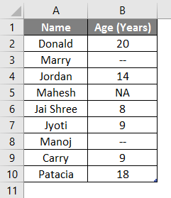
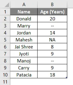
Let’s assume a user has some people’s data like Name and Age, where the user wants to calculate the count of the name with age data in the table.
Let’s see how we can do this with the count function.
Step 1: Open MS Excel from the start menu >> Go to Sheet1, where the user keeps the data.
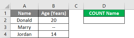
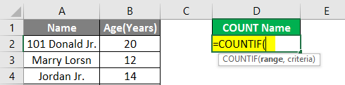
Step 2: Now create headers for the Count name where the user wants the count name, which has age data.
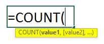
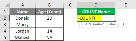
Step 3: Now calculate the count of a name in the given data by the Count function>> use the equal sign to calculate >> Write in D2 Cell and use COUNT>> “=COUNT (”

Step 4: Now, it will ask for the value1 which are given in B2 to B10 cell >> select B2 to B10 cell >> “=COUNT (B2: A10)”
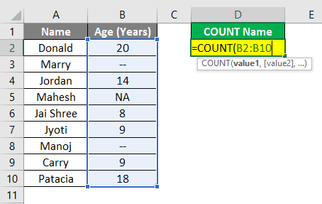
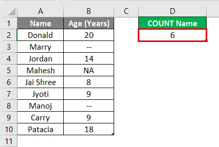
Step 5: Now press the Enter key.
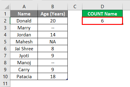
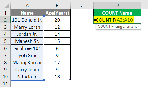
Summary of Example #1: The user wants to calculate the name count, which has age data in the table. So, 6 names in the above example have age data in the table.
Example #2 – Count Name which has Some Common String
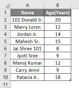
Let’s assume a user has some people’s personal data like Name and Age, where the user wants to calculate the count of the name with the “Jr.” string common in their name. Let’s see how we can do this with the COUNTIF function.
Step 1: Open MS Excel from the start menu >> Go to Sheet2, where the user keeps the data.
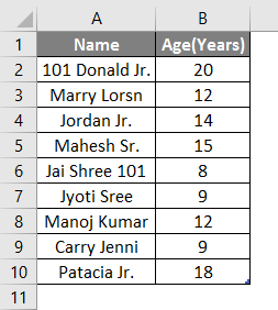
Step 2: Create a header for the Count name, with a “Jr.” string common in their name.
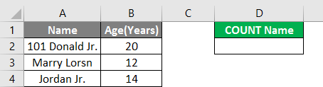
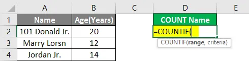
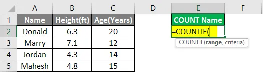
Step 3: Now calculate the count of a name in the given data by the COUNTIF function>> use the equal sign to calculate >> Write in D2 Cell and use COUNTIF>> “=COUNTIF (”
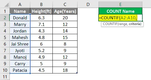
Step 4: Now, it will ask for value1 which are given in A2 to A10 cell >> select A2 to A10 cell >> “=COUNTIF (A2: A10,”
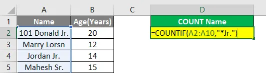
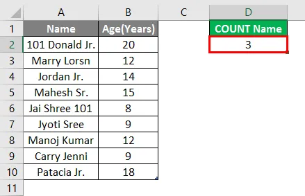
Step 5: Now it will ask for criteria which are to search only for the “Jr.” string in the name >>so write in D2 cell >> “=COUNTIF (A2: A10,” *Jr.”)”

Step 6: Now press the Enter key.

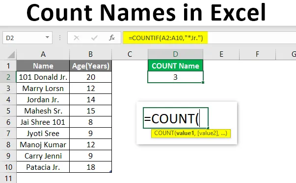
Summary of Example #2: The user wants to count the name with the “Jr.” string common in their name in the table. So, three names in the above example have the “Jr.” string in their name.
Example #3 – Number of Letters with Ending a Specific String
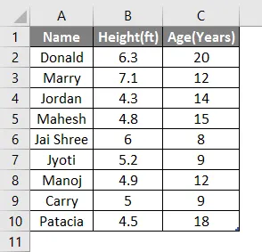
Let’s assume a user wants to count the names with 5 letters and the “ry” string common in their name. Let’s see how we can do this with the COUNTIF function.
Step 1: Open MS Excel from the start menu >> Go to Sheet3, where the user keeps the data.
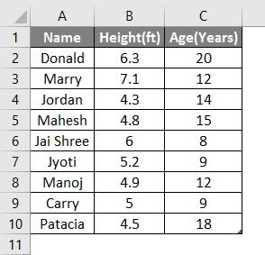
Step 2: Create a header for the Count name, with 5 letters and a “ry” string common in their name.
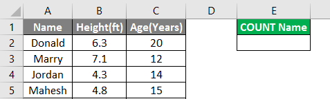
Step 3: Now calculate the count of a name in the given data by the COUNTIF function>> use the equal sign to calculate >> Write in E2 Cell and use COUNTIF>> “=COUNTIF (”
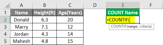
Step 4: Now, it will ask for value1 which are given in A2 to A10 cell >> select A2 to A10 cell >> “=COUNTIF (A2: A10,”

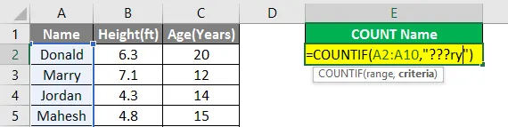
Step 5: Now it will ask for criteria which are to search only for the “ry” string in the name with 5 letters>>so write in E2 cell >> “=COUNTIF (A2: A10,”???ry”)”
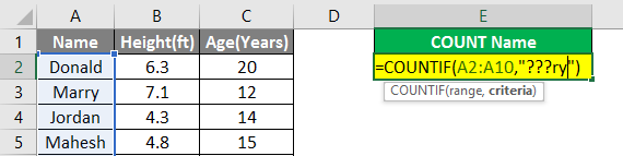
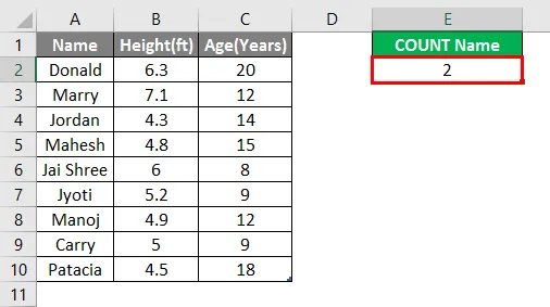
Step 6: Now press the Enter key.
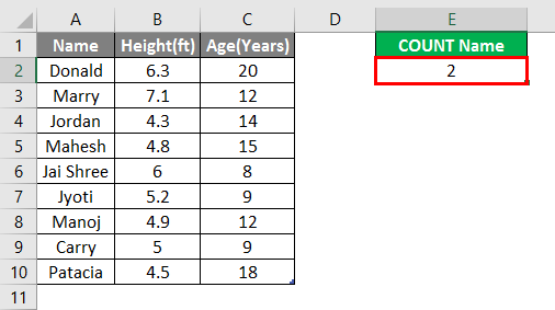
Summary of Example #3: The user wants to count the names with 5 letters in the Name and the “ry” string common in their name in the table. So, 2 names in the above example have a “ry” string in their name with five letters.
Things to Remember About Count Names in Excel
- The Count function comes under the statistical function category and is used to return an integer as output.
- If a cell contains any value that is not numeric, like text or #NA, it will not be counted by the count function.
- The asterisk (*) matches any set of characters in the COUNTIF criteria.
- The question mark (?) is used as the wildcard character to match any single character in the criteria of the function.
- In the criteria, a user can use greater than “>,” less than “<” or equal to the “=” symbol to create criteria in the function. As an example, “=COUNTIF (A2:A5,” >=10″)” here as the output will return the count of the cell, which has a value greater than or equal to 10.
Recommended Articles
This is a guide to Count Names in Excel. Here we discuss How to Count Names in Excel, examples, and a downloadable excel template. You may also look at the following articles to learn more –
- Count Cells with Text in Excel
- Count Characters in Excel
- Count Formula in Excel
- COUNTIFS in Excel
You can use the following methods to count names in Excel:
Method 1: Count Cells with Exact Name
=COUNTIF(A2:A11, "Bob Johnson")
Method 2: Count Cells with Partial Name
=COUNTIF(A2:A11, "*Johnson*")
Method 3: Count Cells with One of Several Names
=COUNTIF(A2:A11, "*Johnson*") + COUNTIF(A2:A11, "*Smith*")
The following examples show how to use each method with the following dataset in Excel:

Example 1: Count Cells with Exact Name
We can use the following formula to count the number of cells in column A that contain the exact name “Bob Johnson”:
=COUNTIF(A2:A11, "Bob Johnson")
The following screenshot shows how to use this formula in practice:

We can see that there are 2 cells that contain “Bob Johnson” as the exact name.
Example 2: Count Cells with Partial Name
We can use the following formula to count the number of cells in column A that contain “Johnson” anywhere in the name:
=COUNTIF(A2:A11, "*Johnson*")
The following screenshot shows how to use this formula in practice:

We can see that there are 4 cells that contain “Johnson” somewhere in the name.
Example 3: Count Cells with One of Several Names
We can use the following formula to count the number of cells in column A that contain “Johnson” or “Smith” somewhere in the name:
=COUNTIF(A2:A11, "*Johnson*") + COUNTIF(A2:A11, "*Smith*")
The following screenshot shows how to use this formula in practice:

We can see that there are 6 cells that contain either “Johnson” or “Smith” somewhere in the name.
Additional Resources
The following tutorials explain how to perform other common tasks in Excel:
How to Count Specific Words in Excel
How to Count Unique Values by Group in Excel
How to Use COUNTIF with Multiple Ranges in Excel
- Обзор имен имен в Excel
Подсчет имен в Excel (Содержание)
- Обзор имен имен в Excel
- Как считать имена в Excel?
Обзор имен имен в Excel
COUNT — это встроенная функция в MS Excel, которая будет подсчитывать количество ячеек, содержащих числа в ячейке. Он относится к категории статистической функции и используется для возврата целого числа в качестве выходных данных. Существует множество способов подсчета ячеек в заданном диапазоне по нескольким критериям пользователя. Например, COUNTIF, DCOUNT, COUNTA и т. Д.
Формула: в простой функции подсчета есть много параметров-значений, где она будет считать все ячейки, содержащие числа.

Есть несколько конкретных встроенных функций Count, которые перечислены ниже:
- COUNT : будет подсчитано количество ячеек, содержащих числа.
- COUNTIF : будет подсчитывать количество ячеек, содержащих числа, и должно соответствовать критериям пользователя.
- DCOUNT : будет подсчитывать ячейки, которые содержат некоторое количество в выбранной базе данных и которые удовлетворяют пользовательским критериям.
- DCOUNTA : будет подсчитывать непустые ячейки в выбранной базе данных, которые удовлетворяют пользовательским критериям.
Как считать имена в Excel?
Подсчет имен в Excel очень прост и легок. Итак, вот несколько примеров, которые могут помочь вам подсчитать имена в Excel.
Вы можете скачать этот шаблон Excel Count Names здесь — Шаблон Excel Count Names
Пример № 1 — Имя счетчика с данными о возрасте
Давайте предположим, что есть пользователь, у которого есть личные данные некоторых людей, такие как Имя и Возраст, где пользователь хочет рассчитать количество имен, у которых есть данные о возрасте в таблице.
Давайте посмотрим, как мы можем сделать это с помощью функции Count.
Шаг 1: Откройте MS Excel из меню Пуск >> Перейдите на Лист1, где пользователь сохранил данные.
Шаг 2: Теперь создайте заголовки для имени счета, где пользователь хочет, чтобы имя счета имело данные о возрасте.

Шаг 3: Теперь вычислите количество имен в данных с помощью функции Count >> используйте знак равенства для вычисления >> Write в ячейке D2 и используйте COUNT >> «= COUNT («
Шаг 4: Теперь будет запрошено значение 1, указанное в ячейке B2 — B10 >> выберите ячейку B2 — B10 >> «= COUNT (B2: A10)»

Шаг 5: Теперь нажмите на клавишу ввода.
Краткое изложение примера № 1: поскольку пользователь хочет вычислить количество имен, для которых в таблице указаны данные о возрасте. Итак, в приведенном выше примере есть 6 имен, у которых есть данные о возрасте в таблице.
Пример # 2 — Имя счетчика, которое имеет некоторую общую строку
Давайте предположим, что есть пользователь, у которого есть личные данные некоторых людей, такие как Имя и Возраст, где пользователь хочет рассчитать количество имен, для которых в имени встречается строка «Jr.». Давайте посмотрим, как мы можем сделать это с помощью функции COUNTIF.
Шаг 1: Откройте MS Excel из меню «Пуск» >> Перейдите на Sheet2, где пользователь сохранил данные.
Шаг 2: Теперь создайте заголовок для имени Count, в имени которого есть строка «Jr.».

Шаг 3: Теперь вычислите количество имен в данных с помощью функции COUNTIF >> используйте знак равенства для вычисления >> Запись в ячейку D2 и используйте COUNTIF >> «= COUNTIF («
Шаг 4: Теперь он запросит значение1, которое указано в ячейке A2 — A10 >> выберите ячейку A2 — A10 >> «= COUNTIF (A2: A10, »

Шаг 5: Теперь он запросит критерии, по которым нужно искать только строку «Jr.» в имени >>, поэтому напишите в ячейке D2 >> «= COUNTIF (A2: A10, « * Jr. »)»
Шаг 6: Теперь нажмите клавишу Enter.
Краткое изложение примера № 2: поскольку пользователь хочет сосчитать имя, для которого в таблице есть строка «Jr.», общая для его имени. Итак, в приведенном выше примере есть 3 имени, в имени которых есть строка «младший».
Пример № 3 — количество букв с окончанием определенной строки
Предположим, что пользователь хочет сосчитать имена, в имени которых есть 5 букв и строка «ry». Давайте посмотрим, как мы можем сделать это с помощью функции COUNTIF.
Шаг 1: Откройте MS Excel из меню «Пуск» >> Перейдите к Sheet3, где пользователь сохранил данные.
Шаг 2: Теперь создайте заголовок для имени Count, в котором есть 5 букв и строка «ry», общая для их имени.

Шаг 3: Теперь вычислите количество имен в данных с помощью функции COUNTIF >> используйте знак равенства для вычисления >> Запись в ячейку E2 и используйте COUNTIF >> «= COUNTIF («
Шаг 4: Теперь он запросит значение1, которое указано в ячейке A2 — A10 >> выберите ячейку A2 — A10 >> «= COUNTIF (A2: A10, »
Шаг 5: Теперь он запросит критерии, по которым нужно искать только строку «ry» в имени с 5 буквами >>, поэтому пишите в ячейку E2 >> «= COUNTIF (A2: A10, « ??? ry ») »
Шаг 6: Теперь нажмите клавишу Enter.
Краткое изложение примера № 3: Поскольку пользователь хочет подсчитать имена, которые имеют 5 букв в имени и строку «ry», общие для их имени в таблице. Итак, в приведенном выше примере есть 2 имени, в имени которых есть строка «ry» с пятью буквами.
Что нужно помнить о количестве имен в Excel
- Функция Count относится к категории статистических функций и используется для возврата целого числа в качестве выходных данных.
- Если ячейка, содержащая какое-либо значение, которое не является числовым, например, текст или # NA, то она не будет учитываться функцией count.
- Звездочка (*) используется для соответствия любому набору символов в критериях COUNTIF.
- Знак вопроса (?) Используется в качестве символа подстановки для соответствия любому отдельному символу в критериях функции.
- В критериях пользователь может использовать больше, чем «>», меньше, чем «= 10»), здесь в качестве выходных данных он будет возвращать счетчик ячейки, значение которой больше или равно 10.
Рекомендуемые статьи
Это руководство по подсчету имен в Excel. Здесь мы обсуждаем, как считать имена в Excel вместе с примерами и загружаемым шаблоном Excel. Вы также можете посмотреть следующие статьи, чтобы узнать больше —
- Как добавить ячейки в Excel
- Кнопка вставки Excel
- Оценить формулу в Excel
- ГОД Формула в Excel
Counting names in excel is an essential skill that you need as a student or business person. Accurate counting is crucial in every industry, whether it’s sales consultancy, accounting, or mission control. A name list can either be useful for a specific function like scheduling or be updated regularly for a large number of people.
Counting names in Excel is often one of the most time-consuming tasks and one of those tasks that you will encounter every other day using excel. In this article, we’ll show you how to count names in excel in an easy and simple way , there are different methods to do that, let us take you through each one by one.
How to count names in excel using the COUNTA function
The COUNTA function is one of the most widely used functions in Excel. It counts how many times a specified value appears in a list. This can be useful for counting names, for example, in a spreadsheet that includes customer names or employee names.
The syntax for the COUNTA function is:
=COUNTA(range)
The COUNTA function counts the number of rows in a specified range. This can be useful to find out how many names and addresses are in a list. To use the COUNT function, you must specify a range that contains at least one cell and contains at least one value.
1.Take an example at the list of names that we want to count and we want our answer in D3 cell.
2.We will select the COUNTA function under statistical formulas provided in formulas tab.
3.Here inside the value1, we enter the range of data we want to count which in our case is from A2 to A7.
4.The result will come in our desired tab i-e D3.
How to count specific names in excel
Sometimes you may be looking for how many times a specific name comes in some list, for this purpose you have to use the COUNTIF function, the syntax of this function is
COUNTIF (Range, match case)
1.Let’s suppose we are looking at a list of how many times John has been awarded the “Employee of the month award in the following list.
2.Select the range of data in the column and apply the COUNTIF function to get the answer.
3.The answer we get here is 2, which means Jake occurs 2 times in our data.
How to count names in excel using the SUMPRODUCT function
Sometimes, you have to take into account both upper- and lower-case characters while counting the names, for this, we use the SUMPRODUCT function, which is used when data is case sensitive like in the case given below.
1.We can see that in our Data Two Henry are present but our concern is with a single one only, we will apply the function as.
2.Inside the formula bar, we have entered the exact value we want to match with and the range of our data.
The answer comes out as 1 as expected.
3.And that’s the SUMPRODUCT method for counting names in excel.
Did you learn about how to count names in excel using different methods You can follow WPS Academy to learn more features of Word Document, Excel Spreadsheets, and PowerPoint Slides.
You can also download WPS Office to edit the word documents, excel, and PowerPoint for free of cost. Download now! And get an easy and enjoyable working experience.
For users who are struggling with handling Microsoft Excel when trying to copy the same name multiple times without making it confusing, a simple procedure needs to be followed in order to count a list of names. A list of names in a report may be generated, where the same name appears multiple times. With column ‘A’ having a list of names, where the same name is repeated, and the user desires to display all the names in column ‘B’, but only once.
With this issue, it is required to use the Filter and Advanced Filter options from the Data menu dropdown list. Using the radio button and the ‘copy-to’ options, it is required to choose the ‘unique records only’ option to solve this issue.
What is an Excel formula to count a list of names?
You have a list of names that will change as reports are generated. The report will include the same name multiple times, so the name joebloggs could appear 10 times. You need a formula to scan COL:A that has the list of names. In COL:B you would like Excel to display each of the different names that are in COL:A but only once. So, for example, JOEBLOGGS would appear in B2 only once. Then in COL:C you would like the total amount of times that name appeared in that list. So for example:
A B C
1 joebloggs JOEBLOGGS 5
2 joebloggs
3 joebloggs
4 joebloggs
5 joebloggs
These names will vary so you cannot specify the names using COUNTIF function. You need Excel to populate the names in B automatically.
Solution
Suppose your data is like this from A1 to A9 (note column heading — this is necessary)
Names
a
a
a
a
s
s
d
d
- Click on Data(menu)-Filter-AdvancedFilter
- Choose radio button at the top «copy to another location»
- Next to the list range click on the icon at the right end of the small window and highlight A1 to A9
- Leave blank criteria range
- Next to «copy to»-click on the icon at the right end of the window and select some empty cell e.g. D1
- Choose «unique records only» at the bottom left
- Click on OK
- you will get D1 to D4 names
Names
a
s
d
in E2 copy paste this formla (repeat E2)
=COUNTIF(A$2:A$9,D2)
copy E2 down.
You will get names frequency
Names
a 4
s 2
d 2
Need more help with Excel? Check out our forum!
Microsoft Word allows you count text, but what about Excel? If you need a count of your text in Excel, you can get this by using the COUNTIF function and then a combination of other functions depending on your desired result.
How to count text in Excel
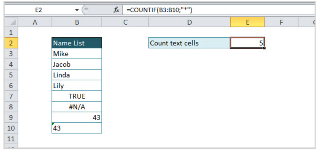
If you want to learn how to count text in Excel, you need to use function COUNTIF with the criteria defined using wildcard *, with the formula: =COUNTIF(range;"*"). Range is defined cell range where you want to count the text in Excel and wildcard * is criteria for all text occurrences in the defined range.
Some interesting and very useful examples will be covered in this tutorial with the main focus on the COUNTIF function and different usages of this function in text counting. Limitations of COUNTIF function have been covered in this tutorial with an additional explanation of other functions such as SUMPRODUCT/ISNUMBER/FIND functions combination. After this tutorial, you will be able to count text cells in excel, count specific text cells, case sensitive text cells and text cells with multiple criteria defined – which is a very good base for further creative Excel problem-solving.
Count Text Cells in Excel
Text Cells can be easily found in Excel using COUNTIF or COUNTIFS functions. The COUNTIF function searches text cells based on specific criteria and in the defined range. As in the example below, the defined range is table Name list, and text criteria is defined using wildcard “*”. The formula result is 5, all text cells have been counted. Note that number formatted as text in cell B10 is also counted, but Booleans (TRUE /FALSE) and error (#N/A) are not recognized as text.
The formula for counting text cells:
=COUNTIF(range;"*")
For counting non-text cells, the formula should be a little bit changed in criteria part:
=COUNTIF(range;"<>*")
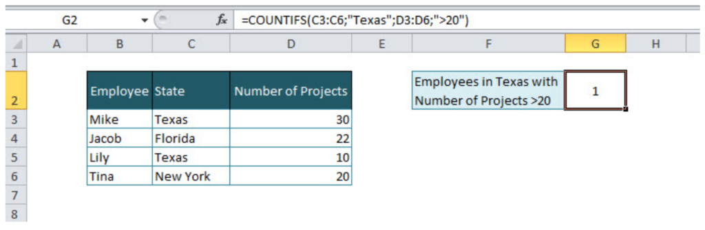
If there are several criteria for counting cells, then COUNTIFS function should be used. For example, if we want to count the number of employees from Texas with project number greater than 20, then the function will look like:
=COUNTIFS(C3:C6;"Texas";D3:D6;">20").
In criteria range in column State, a specific text criteria is defined under quotations “Texas”. The second criteria is numeric, criteria range is column Number of projects, and criteria is numeric value greater than 20, also under quotations “>20”. If we were looking for exact value, the formula would look like:
=COUNTIFS(C3:C6;"Texas";D3:D6;20)
Count Specific Text in Cells
For counting specific text under cells range, COUNTIF function is suitable with the formula:
=COUNTIF(range;"*text*")
=COUNTIF(B3:B9;"*Mike*")
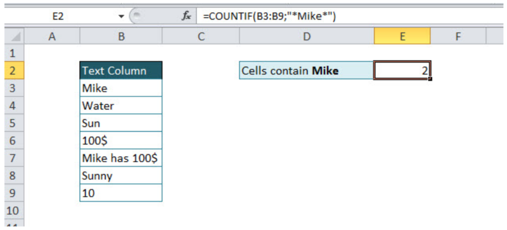
The first part of the formula is range and second is text criteria, in our example “*Mike*”. If wildcard * has not been used before and after criteria text, formula result would have been 1 (Formula would find cells only with word Mike). Wildcard * before and after criteria text, means that all cells that contain criteria characters will be taken into account. As in another example below with text criteria Sun, three cells were found (sun, Sunny, sun is shining)
=COUNTIF(B3:B10;"*Sun*")
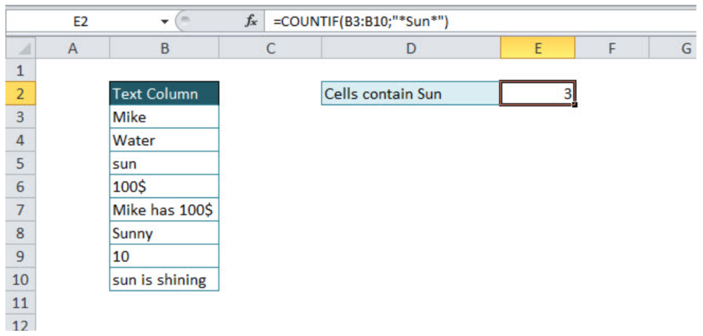
Note: The COUNTIF function is not case sensitive, an alternative function for case sensitive text searches is SUMPRODUCT/FIND function combination.
Count Case Sensitive Specific Text
For a case-sensitive text count, a combination of three formulas should be used: SUMPRODUCT, ISNUMBER and FIND. Let’s look in the example below. If we want to count cells that contain text Sun, case sensitive, COUNTIF function would not be the appropriate solution, instead of this function combination of three functions mentioned above has to be used.
=SUMPRODUCT(--ISNUMBER(FIND("Sun";B3:B10)))
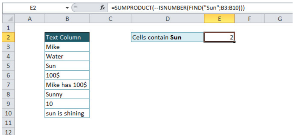
We should go through a separate function explanation in order to understand functions combination. FIND function, searches specific text in the defined cell, and returns the number of the starting position of the text used as criteria. This explanation is relevant, if the searching range is just one cell. If we want to use FIND function in a range of the cells, then the combination with SUMPRODUCT function is necessary.
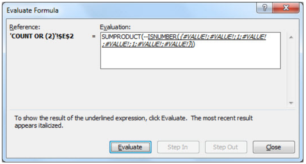
Without ISNUMBER, function combination of FIND and SUMPRODUCT functions would return an error. ISNUMBER function is necessary because whenever FIND function does not match defined criteria, the output will be an error, as in print screen below of the evaluated formula.
In order to change error values with Boolean TRUE/FALSE statement, ISNUMERIC formula should be used (defining numeric values as TRUE, and non-numeric as FALSE, as in print screen below).
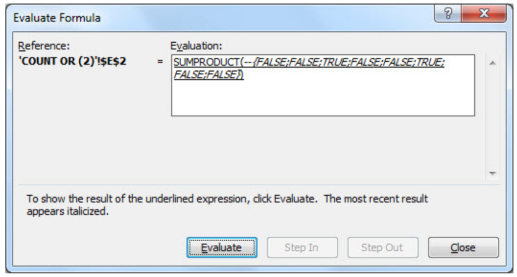
You might be wondering what character — in SUMPRODUCT function stands for. It converts Boolean values TRUE/FALSE in numeric values 1/0, enabling SUMPRODUCT function to deal with numeric operations (without character — in SUMPRODUCT function, the final result would be 0).
Remember, if you want to count specific text cells that are not case sensitive, COUNTIF function is suitable. For all case sensitive searches combination of SUMPRODUCT/ISNUMBER/FIND functions is appropriate.
Count Text Cells with Multiple Criteria
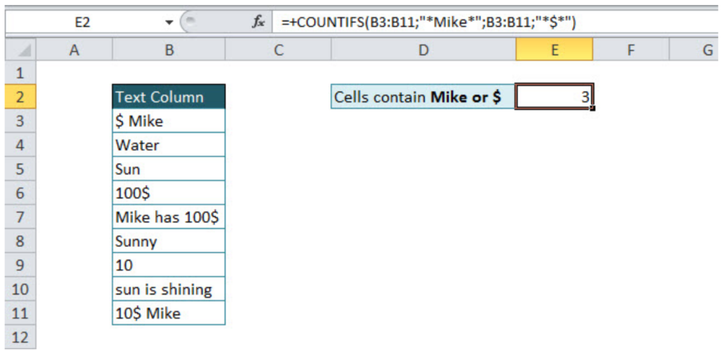
If you want to count cells with Multiple criteria, with all criteria acceptable, there is an interesting way of solving that problem, a combination of SUMPRODUCT/ISNUMBER/FIND functions. Please take a look in the example below. We should count all cells that contain either Mike or $. Tricky part could be the cells that contain both Mike and $.
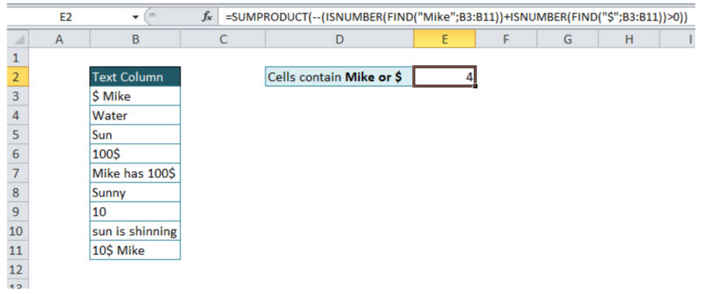
=SUMPRODUCT(--(ISNUMBER(FIND("Mike";B3:B11))+ISNUMBER(FIND("$";B3:B11))>0))
Formula just looks complex, in order to be easier for understanding, I will divide it into several steps. Also, knowledge from the previous tutorial point will be necessary for further work, since the combination of FIND, ISNUMBER, and SUMPRODUCT functions have been explained.
In the first part of the function, we loop through the table and find cells that contain Mike:
=ISNUMBER(FIND("Mike";B3:B11))
The output of this part of the function will be an array with values {1;0;0;0;1;0;0;0;1}, number 1, where criteria have been met, and 0, where has not.
In the second part of the function, looping criteria is $, counting cells containing this value:
=ISNUMBER(FIND("$";B3:B11))
The output of this part of the function will be an array with values {1;0;0;1;1;0;0;0;1}, number 1, where criteria have been met, and 0, where has not.
Next step is to sum these two arrays, since cell should be counted if any of conditions is fulfilled:
=ISNUMBER(FIND("Mike";B3:B11))+ISNUMBER(FIND("$";B3:B11))
The output of this step is {2;0;0;1;2;0;0;0;2}, the number greater than 0 means that one of the condition has been met (2 – both conditions, 1 – one condition)
Without function part >0, the final function would double count cells that met both conditions and the final result would be 7 (sum of all array numbers). In order to avoid it, in the formula should be added >0:
=ISNUMBER(FIND("Mike";B3:B11))+ISNUMBER(FIND("$";B3:B11))>0
The output of this step is array {1;0;0;1;1;0;0;0;1}, the previous array has been checked and only values greater than 0 are TRUE (in an array have value 1), and others are FALSE (in an array have value 0).
Final output of the formula is the sum of the final array values, 4.
Looks very confusing, but after several usages, you will become familiar with this functions.
At the end, we will cover one more multiple criteria text count function, already mentioned in the tutorial, COUNTIFS function. In order to distinguish the usage of functions mentioned above and COUNTIFS function, two words are enough OR/AND. If you want to count text cells with multiple criteria but all conditions have to be met at the same time, then COUNTIFS function is appropriate. If at least one condition should be met, then the combination of function explained above is suitable.
Look at the example below, the number of cells that contain both Mike and $ is easily calculated with COUNTIFS function:
=COUNTIFS(range1;"*text1*";range2;"*text2*")
=COUNTIFS(B3:B11;"*Mike*";B3:B11;"*$*")
In the defined range, function counts only cells where both conditions have been met. The final result is 3.
Still need some help with Excel formatting or have other questions about Excel? Connect with a live Excel expert here for some 1 on 1 help. Your first session is always free.
Excel is great and summing things up. And then count the number of rows easily. You can watch the step by step video on how to use simple functions in Excel.
In fact, most versions of Excel can even show the SUM, COUNT of a block of cells, in the bottom status bar automatically.
However, there is an issue, if you want to count number of employees, or number of departments, or number of students…
Text values, by default can not be summed by the SUM function, and can not be COUNTED by the Count function in Excel
That’s because Excel is good at adding and counting numbers, and not Text. If you try, you’ll get a ZERO.
=COUNT(Employee_Names) will result in a ZERO answer.
Fortunately, the workaround is pretty simple, straight forward and easy to use in Microsoft Excel. And it counts text values with ease.
Instead of using the COUNT function, you can use the COUNTA function of Excel. COUNTA is to count Textual data.
So if you have characters, alphabets and number combinations (like employee numbers), you can count such text items using the COUNTA function of Excel.
This COUNTA Function works in all the versions of Excel – from Excel 2007, Excel 2010, Excel 2013, Excel 2016, Excel 2019, and even Microsoft Office Excel 365 (the cloud version.)
So to count the number of employees, you only need to say =COUNTA(A5:A15).
And this nifty function will count the number of employees promptly. COUNTA is to count Alphanumeric values – text, strings… or even numbers.
Try it out, and let me know if this helps you… 🙂
You may find these resources useful:
- View all Formulas in Excel in a Single Click
- How to Build a Two Axis Chart in Excel
Cheers,
Vinai Prakash
Founder of ExcelChamp.Net
P.S. – Are you an Expert in using Excel ? Try solving this – find a way to find duplicates in Excel 2010 quickly. And post your solution. We are looking for simple and innovative ways to do so…