Excel count by month

There are a handful of functions that we can use to count by date, month, year, or date range in Excel 365.

We can use Excel functions such as COUNTIF, COUNTIFS, SUMPRODUCT, or combinations such as IF + SUM or COUNT + FILTER for this.

But I would pick the former two functions in Excel 365. Do you know why?

Dynamic array formulas, which spill results, are one of the main attractions in Excel in Microsoft 365.

If you are looking for a dynamic array formula to count by date, month, year, and date range in Excel 365, pick none other than COUNTIF/COUNTIFS.

So, in this tutorial, let’s learn to use COUNTIF or COUNTIFS to count by date, month, year, and date range and return an array result.

Sample Records

I have extracted a few records from my daily expense spreadsheet.

Of course, I have sanitized the data to avoid sharing personal info/preferences.

So it’s just a mockup of data in Excel 365. In that, we can try to use COUNTIF and COUNTIFS to count by date, month & year, month, year, and date range.

We will try conditions (criteria) in single (non-array) and multiple (array) rows.

At one instance, we will use a helper column, and that is for the count by month (not month and year).

Sample Data:

COUNTIF to Count by a Specific Date in Excel 365

Countif Syntax: COUNTIF(range,criteria)

Non-Array Formula (Single Date)

How to search and count the number of transactions on a particular date in the above records?

Criterion/Condition: 01/06/2020 (cell F2)

Formula:-

Insert the below Excel COUNTIF formula in cell G2 to count by the specific date, i.e., 01/06/2020.

=COUNTIF(A2:A22,F2)

The above Excel formula searches F2 date in A2:A22 and returns the count, i.e., 2.

Array Formula (Multiple Dates)

Can we use multiple dates (criteria) to count in the above Excel 365 formula?

Yes. Here is how.

Criteria/Conditions: 02/06/2020 (cell F4) and 01/07/2020 (cell F5).

Formula:-

Insert the below Excel COUNTIF formula in cell G4 to count by the specific dates, i.e., 02/06/2020 and 01/07/2020. It will automatically spill in G5.

=COUNTIF(A2:A22,F4:F5)

COUNTIFS to Count by Month and Year in Excel 365

COUNTIFS Syntax: COUNTIFS(criteria_range1,criteria1, ...)

The functions COUNTIF and COUNTIFS in Excel 365 won’t take other functions in their ‘range’.

So we can’t use month(range)= within these two functions.

But they support other functions in the criteria part, and we will try to benefit from that feature below.

Non-Array Formula (Month and Year)

We can use COUNTIFS to count by month and year in Excel 365.

Criterion/Condition: 6 (cell F8) and 2020 (cell G8).

Formula:-

Insert the below Excel COUNTIFS formula in cell H8 to count by the above month and year.

=COUNTIFS(A2:A22,">="&DATE(G8,F8,1),A2:A22,"<="&EOMONTH(DATE(G8,F8,1),0))

The DATE(G8,F8,1) formula returns 01/06/2020, and EOMONTH(DATE(G8,F8,1)) returns the last date in that month.

The count of dates between these dates will be equal to the count by month and year.

Array Formula (Months and Years)

We can use multiple months and years (criteria) in the above Excel 365 formula.

Criteria/Conditions:

1. 7 (cell F10) and 2020 (cell G10).
2. 7 (cell F11) and 2021 (cell G11).

Formula:-

Insert the below Excel COUNTIFS formula in cell H10 to count by the above multiple months and years.

=COUNTIFS(A2:A22,">="&DATE(G10:G11,F10:F11,1),A2:A22,"<="&EOMONTH(DATE(G10:G11,F10:F11,1),0))

Array and Non-Array COUNTIFS to Count by Year in Excel 365

Assume we have the year 2020 in cell F14.

The following COUNTIFS non-array in cell G14 returns the count by the provided year in Excel 365.

=COUNTIFS(A2:A22,">="&DATE(F14,1,1),A2:A22,"<="&DATE(F14,12,31))

If the year 2020 is in cell F16 and 2021 is in cell F17, then we can use the below Excel 365 dynamic array formula in cell G16.

=COUNTIFS(A2:A22,">="&DATE(F16:F17,1,1),A2:A22,"<="&DATE(F16:F17,12,31))

I hope, the above two Excel formulas are self-explanatory. Let’s move to the next example.

Array and Non-Array COUNTIFS to Count by Date Range in Excel 365

In the above examples, we have learned to count the number of transactions that have taken place on a specific date, month, and year.

But what about counting the number of transactions between two dates in Excel 365?

I wish to know how many transactions I have done during 01/06/2020 (F20) and 06/06/2020 (G20).

I can use the below Excel formula in cell H20 for that.

Count by Date Range Non-Array Formula (H20):

=COUNTIFS(A2:A22,">="&F20,A2:A22,"<="&G20)

What about a count by date range array formula?

Date Range 1: F22:G22

Date Range 2: F23:G23

Count by Date Range Array Formula (H22):

=COUNTIFS(A2:A22,">="&F22:F23,A2:A22,"<="&G22:G23)

Array and Non-Array COUNTIFS to Count by Month Alone in Excel 365

I know this is a rare scenario.

Usually, we may include the year component in such calculations.

For example, we will usually find the number of sales in January 2020, not in both January 2020 and January 2021.

But if you are very particular to use COUNTIFS to count by month only in Excel 365, follow the below steps.

Insert the below formula in cell D2. It will substitute the year part of the dates in cell A2:A22 with the year 2021.

=DATE(2021,MONTH(A2:A22),1)

It’s a dynamic array (spill) formula. So it requires a blank range in D3:D22.

You can then hide column D or keep it.

In cell K8, enter 6 which represents June.

=COUNTIFS(D2#,">="&DATE(2021,J10,1),D2#,"<="&EOMONTH(DATE(2021,J10,1),0))

The above formula in cell L8 will return the count of transactions in June. It ignores the years!

What about an array formula?

Enter 6 in K10 and 7 in K11. Then, you may insert the below formula in L10.

=COUNTIFS(D2#,">="&DATE(2021,K10:K11,1),D2#,"<="&EOMONTH(DATE(2021,K10:K11,1),0))

Excel 365 Resources

• Running Count Array Formula in Excel 365.
• Array Formula to Conditional Count Unique Values in Excel 365.
• Split Function Alternative in Excel 365 with Multi-Row Support.
• How to Flatten an Array in Excel 365 Using Dynamic Formulas.
• Spill Formulas to Sum Each Row in Excel 365.

EXPLANATION

This tutorial shows how to count the number of occurrences by month through the use of an Excel formula or VBA.

The Excel method uses a combination of Excel SUMPRODUCT and MONTH functions to count by month. The MONTH function is used to identify the nominated month from a range of dates and the SUMPRODUCT then sums all of the occurrences.

The VBA method uses the MONTH VBA function and loops through the range of dates to identify which of the dates contain the relevant month. If a date contains the specified month the VBA code will add 1 to the counter and once it has looped through the entire range it will return the total number of occurrences.

FORMULA
=SUMPRODUCT((MONTH(date_range)=month_value)*(MONTH(date_range)=month_value))

ARGUMENTS
date_range: The range of cells that contain the dates.
month_value: The value that represents the month that you want to count for.

This post will guide you how to create a summary count by month with COUNTIFS function in Excel 2013/2016 or Excel office 365. You can use the COUNTIF function to count cells with a given criteria in excel. this guide will show you the simple formula used to create a summary count by month with COUNTIFS function and the EDATE function with two criteria in Excel.

---

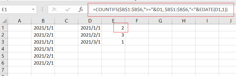
Assuming you have a list of data in range B1:B6 that contain date values, and you want to get a total count per month in your summary table(D1:D3) in your worksheet, and you can use a formula based on the COUNTIFS function to generate a total count per month. Like this:

=COUNTIFS($B$1:$B$6,">="&D1, $B$1:$B$6,"<"&EDATE(D1,1))

Let’s See How This Formula works:

The COUNTIFS function can be used to count the number of cells that meet multiple conditions or criteria. And the Cell D1 is a date for the first of each month in 2021. And if you want to generate a total count per month, and you need to provide criteria that will filter all the date values that appear in each month in range B1:B6.

You still need to build criteria that is a second date can be created with the EDATE function. It means that dates must be greater than or equal to the data in cell D1 or less than the data in D1 plus one month (get it with EDATE function).

---

• Excel COUNTIFS function
  The Excel COUNTIFS function returns the count of cells in a range that meet one or more criteria. The syntax of the COUNTIFS function is as below:= COUNTIFS(criteria_range1, criteria1, [criteria_range2, criteria2]…)…
• Excel COUNTIF function
  The Excel COUNTIF function will count the number of cells in a range that meet a given criteria. This function can be used to count the different kinds of cells with number, date, text values, blank, non-blanks, or containing specific characters.etc.= COUNTIF (range, criteria)…
• Excel EDATE function
  TThe Excel EDATE function returns the serial number that represents the date that is a specified number of months before or after a specified date.The syntax of the EDATE function is as below:=EDATE (start_date, months)…

In this article, we will learn how to count birth dates from range by month Excel.

While working with dates, we may get the need to count the birth days which belong to the same month. In that case, this excel formula will easily let you know the count of birthdays, in a specific month.

How to solve the problem?

For this article we will use the SUMPRODUCT function. Here we are given birth dates in a range of data and specific monthly values. We need to count the date values where the formula includes all the date values of the given month.

Generic formula:

range : birth date values given in as range

m_value : month number.

Example:

All of these might be confusing to understand. So, let’s test this formula via running it on the example shown below.

Here we have the birth date records and we need to find the date values lying in a specific month or return the count rows where the date value lies within a given month number.

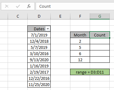
Firstly, we need to define the named range for birthdates range as range. Just select the date values and type the name (range) for the range in the top left corner.

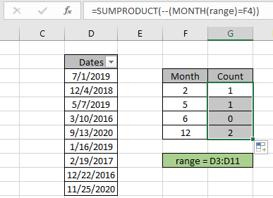
Now we will use the following formula to get a count of the dates which lay in the 2nd month which is February.
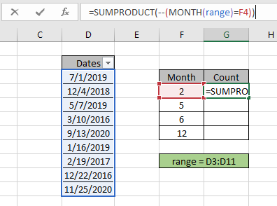
Use the Formula:

= SUMPRODUCT ( — ( MONTH ( range ) = F4 ) )

range : named range used for birth date values D3:D11.

F4 : month value given as cell reference.

= : operator, condition given as equals to sign.

Explanation:

• MONTH ( range ) function extracts the monthly value from the birth date and matches it with the given month number and operator.

= SUMPRODUCT ( — ( { 7 ; 12 ; 5 ; 3 ; 9 ; 1 ; 2 ; 12 ; 11 } = 2 ) )

• = operator matches it with month value 2 and returns an array TRUE and FALSE values depending on the operation.

= SUMPRODUCT ( — { FALSE ; FALSE ; FALSE ; FALSE ; FALSE ; FALSE ; TRUE ; FALSE ; FALSE } )

• — operator used to convert TRUE value to 1 & False value to 0.

= SUMPRODUCT ( { 0 ; 0 ; 0 ;  0 ; 0 ; 0 ; 1 ; 0 ; 0 } )

• SUMPRODUCT function gets the sum of 1s in the returned array, which will be the count of required birth dates.

Here the year value is given as cell reference and range is given as cell reference. Press Enter to get the count.

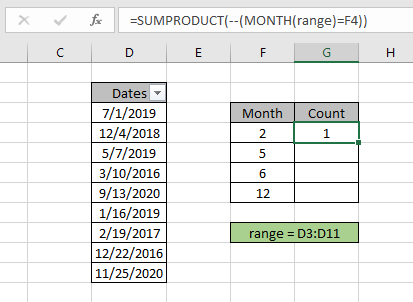
As you can see the total date matches the 2 as month value comes out to be 1. It means there are 1 birthdate in the month of February.
Now copy and paste the formula to other cells using the CTRL + D or drag down option of Excel.

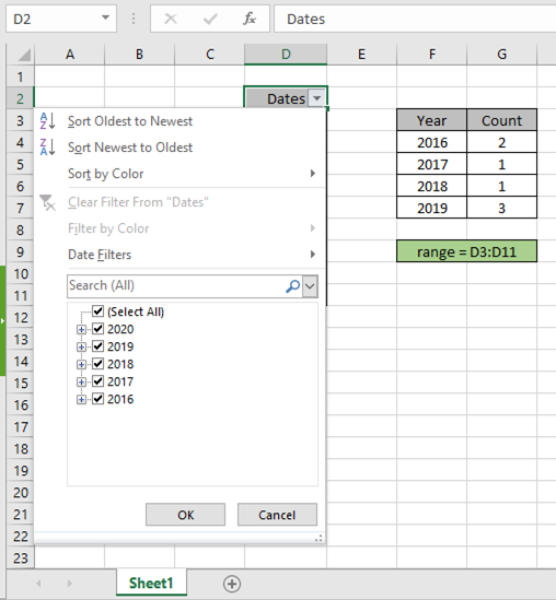
As you can see in the above snapshot we obtain all the date values which lays in a specific year using the Excel formula. You can also obtain check the same using the excel filter option. Apply the filter to the Dates header and deselect the select all option.

For the month of February, select the Date filter option > All dates in this period > February to get the dates as shown below.

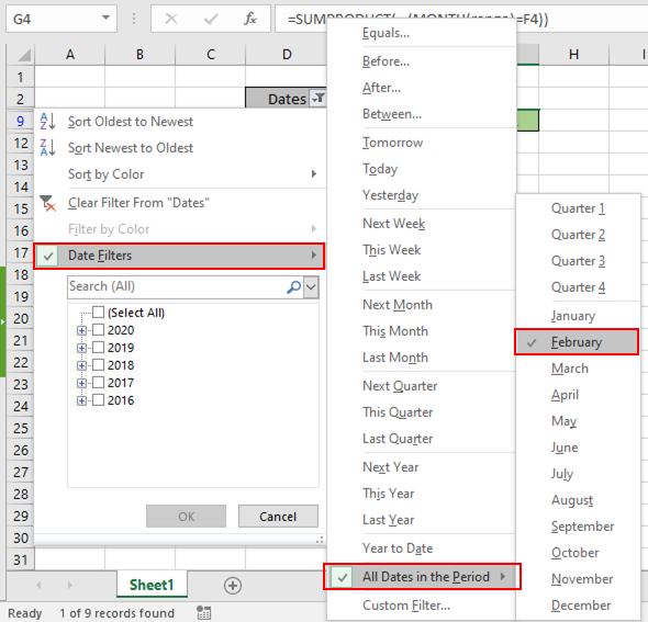
After selecting the filtered dates by month, the dates will be like as shown in the snapshot below.

The filter option returns 1 value as result. Perform the same to other date values to get the count of dates or rows having criteria as given specific year.

Here are some observational notes shown below.
Notes:

1. The formula only works with numbers.
2. The SUMPRODUCT function considers non — numeric values as 0s.
3. The SUMPRODUCT function considers logic value TRUE as 1 and False as 0.
4. The argument array must be of the same length else the function.

Hope this article about how to Return Count if with SUMPRODUCT in Excel is explanatory. Find more articles on SUMPRODUCT functions here.

If you liked our blogs, share it with your friends on Facebook. And also you can follow us on Twitter and Facebook. We would love to hear from you, do let us know how we can improve, complement or innovate our work and make it better for you. Write us at info@exceltip.com

Related Articles

How to use the SUMPRODUCT function in Excel: Returns the SUM after multiplication of values in multiple arrays in excel.

COUNTIFS with Dynamic Criteria Range : Count cells dependent on other cell values in Excel.

COUNTIFS Two Criteria Match : Count cells matching two different criteria on list in excel.

COUNTIFS With OR For Multiple Criteria : Count cells having multiple criteria match using the OR function.

The COUNTIFS Function in Excel : Count cells dependent on other cell values.

How to Use Countif in VBA in Microsoft Excel : Count cells using Visual Basic for Applications code.

How to use wildcards in excel : Count cells matching phrases using the wildcards in excel

Popular Articles

50 Excel Shortcut to Increase Your Productivity

Edit a dropdown list

Absolute reference in Excel

If with conditional formatting

If with wildcards

Vlookup by date

Convert Inches To Feet and Inches in Excel 2016

Join first and last name in excel

Count cells which match either A or B

To count by month has nothing different than How to COUNT values between two dates. However, this article shows you a more dynamic and specialized way with EOMONTH function that you don’t need to guess how many days in a month to count month.

If you only want to calculate the number of days in a month, please refer to this article: How to find number of days in month

Syntax

=COUNTIFS(

  date range,

  «>=» & first day of month,

  date range,

  «<=» & EOMONTH(

    first day of month,

    0

  )

)

Steps

1. Start with =COUNTIFS(
2. Continue with first criteria range – criteria pair with date range and 1^st day of month $B$3:$B$12,»>=»&$D3,
3. Enter second criteria range – criteria pair with date range and EOMONTH function $B$3:$B$12,»<=»&EOMONTH($D3,0)
4. Type ) to close COUNTIFS function and press Enter to complete the formula

How

First of all, the COUNTIFS function counts values that meet single or multiple criteria. Ability to use criteria with logical operators like greater than or equal (>=) and less than or equal (<=) provides the way of counting values between specific values.

To filter dates in a month, we need dates for the first and last days of that specific month. Although the first day of the month is easy to guess. But displaying a particular month like 11/1/2018 is not a preferred approach. Thanks to formatting options in Excel, we can display a full date as month name only. Adding custom format «mmmm» to a date displays it as a long month name without changing its value. To apply a custom format:

1. Select the cell to be formatted and press Ctrl+1 to open the Format Cells dialog. An alternative way to do is by right-clicking the cell and then going to Format Cells > Number Tab.
2. Under Category, select Custom.
3. Type in the format code into the Type
4. Finally, click OK to save your changes.

For detailed information on Number Formatting please visit: Number Formatting in Excel – All You Need to Know.

After adding the first days of months, under a formatting of month names, it is time to enter criteria range-criteria pairs. The first pair is easy: date range and the date of the first day of the month.

$B$3:$B$12,»>=»&$D3,

Next criteria range-criteria pair is the last of the month. We use the EOMONTH function that returns the date for the last day of a month. The EOMONTH gets date and month arguments. The date is the same date we use for first criteria and month argument gets 0 to point exact date in the first argument.

$B$3:$B$12,»<=»&EOMONTH($D3,0)

Now that both criteria range-criteria pairs are set, it is time to use them in the COUNTIFS function to count month.

=COUNTIFS($B$3:$B$12,»>=»&$D3,$B$3:$B$12,»<=»&EOMONTH($D3,0))

В Excel мы можем использовать функцию СЧЁТЕСЛИМН для подсчета ячеек с заданными критериями. В этом руководстве показано, как использовать эту функцию СЧЁТЕСЛИМН вместе с функцией ДАТАФИКАЦИЯ для создания итогового подсчета по месяцам в Excel.

---

Создайте сводный счет по месяцам с помощью функций СЧЁТЕСЛИМН и ДАТА

Чтобы создать итоговый счетчик по месяцам, вы можете использовать формулу, основанную на функциях СЧЁТЕСЛИМН и ДАТАМ, общий синтаксис:

=COUNTIFS(date_range,»>=»&first_day_of_month,date_range,»<«&EDATE(first_day_of_month,1))

• date_range: Список дат, которые вы хотите подсчитать;
• first_day_of_month: Ячейка, содержащая первый день месяца.

Предполагая, что у вас есть список дат в столбце A, теперь вы хотите получить общее количество, основанное на некоторых конкретных месяцах. В этом случае вы должны ввести первые дни месяцев, которые вы хотите посчитать, как показано на скриншоте ниже:

Затем примените следующую формулу в пустую ячейку, чтобы записать результат:

=COUNTIFS($A$2:$A$13,»>=»&C2,$A$2:$A$13,»<«&EDATE(C2,1))

Затем перетащите дескриптор заполнения, чтобы скопировать эту формулу в другие нужные ячейки, и сразу будет возвращено общее количество ячеек, принадлежащих определенному месяцу, см. Снимок экрана:

---

Пояснение к формуле:

=COUNTIFS($A$2:$A$13,»>=»&C2,$A$2:$A$13,»<«&EDATE(C2,1))

• Функция СЧЁТЕСЛИМН используется для подсчета количества ячеек на основе нескольких критериев, в этой формуле C2 — это первый день месяца.
• Чтобы получить общее количество за месяц, вам необходимо указать еще один критерий — первый день следующего месяца. Это можно вернуть с помощью функции EDATE.
• Вся формула означает, что подсчитываемые даты должны быть больше или равны дате в ячейке C2 и меньше первого дня следующего месяца, предоставленного функцией EDATE.

---

Используемая относительная функция:

• COUNTIFS:
• Функция СЧЁТЕСЛИМН возвращает количество ячеек, соответствующих одному или нескольким критериям.

• EDATE:
• Функция СЧЁТЕСЛИМН возвращает серийный номер, который равен n месяцам в будущем или прошлом.

---

Другие статьи:

• Подсчитать количество дат по году, месяцу
• При работе с листом Excel иногда вам может потребоваться подсчитать ячейки, в которых указаны даты за определенный год или месяц, как показано ниже. Чтобы решить эту задачу в Excel, вы можете использовать функции СУММПРОИЗВ, ГОД и МЕСЯЦ для создания формул для подсчета количества дат, принадлежащих определенному году или месяцу, как вам нужно.

• Подсчитать количество ячеек между двумя значениями / датами
• Вы когда-нибудь пытались получить или подсчитать количество ячеек между двумя заданными числами или датами в Excel, как показано на скриншоте ниже? В этой статье мы расскажем о некоторых полезных формулах для решения этой проблемы.

• Количество ячеек, содержащих числовые или нечисловые значения
• Если у вас есть диапазон данных, который содержит как числовые, так и нечисловые значения, и теперь вы можете подсчитать количество числовых или нечисловых ячеек, как показано на скриншоте ниже. В этой статье я расскажу о некоторых формулах решения этой задачи в Excel.

---

Лучшие инструменты для работы в офисе

Kutools for Excel — Помогает вам выделиться из толпы

Хотите быстро и качественно выполнять свою повседневную работу? Kutools for Excel предлагает 300 мощных расширенных функций (объединение книг, суммирование по цвету, разделение содержимого ячеек, преобразование даты и т. д.) и экономит для вас 80 % времени.

• Разработан для 1500 рабочих сценариев, помогает решить 80% проблем с Excel.
• Уменьшите количество нажатий на клавиатуру и мышь каждый день, избавьтесь от усталости глаз и рук.
• Станьте экспертом по Excel за 3 минуты. Больше не нужно запоминать какие-либо болезненные формулы и коды VBA.
• 30-дневная неограниченная бесплатная пробная версия. 60-дневная гарантия возврата денег. Бесплатное обновление и поддержка 2 года.

---

Вкладка Office — включение чтения и редактирования с вкладками в Microsoft Office (включая Excel)

• Одна секунда для переключения между десятками открытых документов!
• Уменьшите количество щелчков мышью на сотни каждый день, попрощайтесь с рукой мыши.
• Повышает вашу продуктивность на 50% при просмотре и редактировании нескольких документов.
• Добавляет эффективные вкладки в Office (включая Excel), точно так же, как Chrome, Firefox и новый Internet Explorer.

Комментарии (0)

Оценок пока нет. Оцените первым!