
Home / Excel Formulas / Count Between Two Numbers (COUNTIFS)
In Excel, you can count between two numbers using the COUNTIFS function. With the COUNTIFS function, you can specify an upper limit of the numbers, and a lower limit to create a range of numbers to count. In the following example, we have a list of names with age. Now we need to count the people of two ages i.e., two numbers.
sample-file

You can use the following steps to create formulas using the COUNTIFS to count numbers between 10 and 25.
- First, enter the “=COUNTIS(“ in cell C1.

- After that, refer to the range from where you want to count the values.

- Next, you need to specify the upper number using greater than and equal sign.

- From here, again you need to refer to the range of numbers in the criteria2.

- In the end, use lower than and equal signs to specify number below than 10 in the counting range.


=COUNTIFS(B2:B26,"<=25",B2:B26,">=10")COUNTIFS can take multiple criteria and count values based on them, and to understand this formula, we need to split it into two parts.

- First, you have specified the range from which you want to count the numbers and the upper number using the greater than and equal signs.
- After that, you specified the lower number and the range of numbers.
sample-file
Using SUMPRODUCT to Count Cells Between Two Numbers
You can also use the SUMPRODUCT function for counting the number of cells between two numbers. In this formula, we need to use the INT function along with the SUMPRODUCT. See the formula below:
=SUMPRODUCT(INT(B2:B26>=10), INT(B2:B26<=25))
To understand the formula, we need to split it:
In the first INT function, we have used the range of cells from where we want to count the numbers. And >= signs to only refer to the numbers greater than or equal to 10. And it returns an array showing all the numbers above 10 using 1.

And in the second INT function, again you have the same range that considers the numbers lower than and equal to 25.

With both INT functions, you have two different arrays. In the first, you have 1 for each number that is greater than or equal to 10, and in the second, 1 for the values which are lower than or equal to 25.

In the end,
- SUMPRODUCT multiplies each value from the first array with the value from the second array, and you will get an array of values that represents numbers that are between 10 and 25.
- And after that return the sum of those values from the array.
sample-file
In this example, the goal is to count numbers that fall within specific ranges. The lower value comes from the «Start» column, and the upper value comes from the «End» column. For each range, we want to include both the lower value and the upper value. For convenience, the numbers being counted are in the named range data (C5:C16). This problem can be solved with both the COUNTIFS function and the SUMPRODUCT function, as explained below.
COUNTIFS function
In the example shown, the formula used to solve this problem is based on the COUNTIFS function, which is designed to count cells that meet multiple criteria. The formula in cell G5, copied down, is:
=COUNTIFS(data,">="&E5,data,"<="&F5)
COUNTIFS accepts criteria in range/criteria pairs. The first range/criteria pair checks for values in data that are greater than or equal to (>=) the «Start» value in column E:
data,">="&E5
The second range/criteria pair checks for values in data that are less than or equal to (<=) the «End» value in column F:
data,"<="&F5
Because we supply the same range (data) for both criteria, each cell in data must meet both conditions in order to be included in the final count. Note in both cases, we need to concatenate the cell reference to the logical operator. This is a quirk of RACON functions in Excel, which use a different syntax than other formulas.
As the formula is copied down column G, it returns the count of numbers that fall in the range defined by columns E and F.
SUMPRODUCT alternative
Another option for solving this problem is the SUMPRODUCT function with a formula like this:
=SUMPRODUCT((data>=E5)*(data<=F5))
This is an example of using Boolean logic. Because there are 12 values in the named range data, each logical expression inside SUMPRODUCT generates an array that contains 12 TRUE and FALSE values. The expression:
data>=E5
returns:
{TRUE;TRUE;TRUE;TRUE;TRUE;TRUE;TRUE;TRUE;TRUE;TRUE;TRUE;TRUE}
And the expression:
data<=F5
returns:
{TRUE;FALSE;FALSE;FALSE;TRUE;FALSE;FALSE;FALSE;TRUE;FALSE;TRUE;FALSE}
When these two arrays are multiplied together, the math operation causes TRUE values to be coerced to 1 and FALSE values to be coerced to zero. The result is a single array of 1s and 0s like this:
=SUMPRODUCT({1;0;0;0;1;0;0;0;1;0;1;0})
Each 1 corresponds to a number in data that meets both conditions and each 0 represents a number that fails at least one condition. With only a single array to process, SUMPRODUCT returns the sum of the numbers in the array, 4, as a final result.
Video: Boolean logic in Excel
Benefits of standard syntax
The nice thing about SUMPRODUCT is that it will handle array operations natively (no need to enter with control + shift + enter) and will accept the more standard syntax for logical expressions seen above. The standard syntax is more useful in other modern formulas. For example you could use the same exact logic with the FILTER function to return the actual numbers that meet these same conditions:
=FILTER(data,(data>=E5)*(data<=F5))
Becomes:
=FILTER(data,{1;0;0;0;1;0;0;0;1;0;1;0})
And FILTER returns the numbers greater than or equal to 70 and less than or equal to 79:
{79;77;75;70}
Video: Basic FILTER function example
When analyzing data in Excel, we sometimes need to know how many numbers appear between two numbers.
For people who work with large datasets, this is a common task.
Manually counting is time-consuming and error-prone.
Excel has a couple of functions that allow us to easily count the number of cells that contain a value between two given numbers.
In this article, you will learn several methods for counting numbers between two numbers in Excel.
Method 1 – Use COUNTIFS Function to Count Between two Numbers in Excel
To count between two numbers in Excel, we can use the COUNTIFS function.
I have the below data set where column A shows the employee names and column B shows the experience of employees in years.
Now I need to find how many employees with 5 to 10 years of experience.

You can use the below function to find the number of employees with 5 to 10 years of experience.
=COUNTIFS(B2:B11,">=5",B2:B11,"<=10")

The syntax of the COUNTIFS function is COUNTIFS(criteria_range1,criteria1,criteria_range2,criteria2,…).
For Criteria_range1, we have to select the range where we need to evaluate the 1st criteria. So, we are selecting cells B2 to B11.
Then, we have to enter the criteria for the 1st range. Our 1st criterion is to have years of experience greater than or equal to 5.
So, enter “>=5”. Here, we have entered the criteria within quotes because we have used a logical operator to define the criteria.
Similarly, we can enter multiple criteria ranges with their respective criteria. So, we select cells B2 to B11 as the 2nd criteria range and enter “<=10” as the criteria for the second range.
Note: When selecting subsequent ranges for criteria, they must have the same number of rows and columns as the 1st criteria range. Otherwise, it will return a #VALUE! Error.

Also read: How to COUNTIF Partial Match in Excel?
Method 2 – Using SUM and IF Functions to Count Between two Numbers in Excel
Another easy way to count between two numbers is to use the combination of SUM and IF functions.
I have the below data set where column A shows the employee names and column B shows the experience of employees in years.
Now I need to find how many employees with 5 to 10 years of experience.

Approach #1 – Multiply two IF functions
You can use the below function to find the number of employees with 5 to 10 years of experience.
=SUM(IF(B2:B11>=5,1,0)*IF(B2:B11<=10,1,0))

The syntax of the IF function is IF(logical_test,[value_if_true],[value_if_false].
Therefore, we are evaluating experience greater than or equal to 5 years with the first IF function.
The value will receive “True” if the experience value is more than or equal to 5, and “False” otherwise. Then, if the logical test result is “True,” we say the function to return 1.
If the logical test returns “False,” we specify that we want to receive “0.”
We are checking the experience of less than or equal to 10 years with the second IF function.
The result will be “True” if the value is less than or equal to 10, and “False” otherwise.
So, if the outcome of the logical test is “True,” we tell the function to return 1. If the logical test returns “False,” we say that we want to receive “0.”
Next, we multiply the corresponding results of two IF functions using the asterisk (*) sign.
This gives an array of numbers where it would be 1 if both corresponding values in both the IF function are 1. Otherwise, we will get 0.
Finally, we use the SUM function to get the total value of the multiplied results.
In this case, the SUM function will help to get the total value of the corresponding multiplied results of the two IF functions.
Approach #2 – Nested IF functions
You can use the below function to find the number of employees with 5 to 10 years of experience.
=SUM(IF(B2:B11>=5,IF(B2:B11<=10,1,0),0))

The syntax of the IF function is IF(logical_test,[value_if_true],[value_if_false].
So, the first IF function is used to test whether the experience is greater than or equal to five years.
It will be “True” if the value is more than or equal to 5, and “False” otherwise.
If the outcome of the logical test is “True,” we then provide the function to assess another IF function. If the logical test returns “False,” we specify to get “0.”
We are evaluating whether the experience is less than or equal to 10 years by using the inner IF function.
If the value is less than or equal to 10, the inner IF function will get “True” and otherwise “False”.
Then, if the outcome of the logical test of the inner IF function is “True,” we tell the function to return 1.
If the logical test of the inner IF function returns “False,” we specify to get “0.”
Therefore, we only receive 1 if the logical tests of both IF functions are True. If not, we shall get 0.
Finally, we use the SUM function to get the total value of the results.
In this case, the SUM function will help to get the total value of the results of the nested IF function.
Method 3 – Using SUMPRODUCT Function to Count Between two Numbers in Excel
You can use the SUMPRODUCT function also to count between two numbers in Excel.
I have the below data set where column A shows the employee names and column B shows the experience of employees in years.
Now I need to find how many employees with 5 to 10 years of experience.

You can use the below function to find the number of employees with 5 to 10 years of experience.
=SUMPRODUCT((B2:B11>=5)*(B2:B11<=10))

The syntax of the SUMPRODUCT function is SUMPRODUCT(array1, [array2], [array3], …).
Now we will check how we have used this function for our calculation.
The first expression (B2:B11>=5) is a logical test. It will check whether or not the values are greater than or equal to 5.
The formula will return “True” if the value is greater than or equal to 5, and “False” otherwise.
The second expression (B2:B11<=10) is also a logical test. It will evaluate whether or not the values are less than or equal to 10.
The formula will return “True” if the value is less than or equal to 10, and “False” otherwise.
The asterisk sign (*) in between the two logical expressions will convert True and False values to 1’s and 0’s and multiply the corresponding values.
When two related numbers are multiplied, the formula returns 1 if both corresponding values are 1, otherwise, it returns 0.
Finally, we use the SUMPRODUCT function to get the sum of the above-multiplied results.
Method 4 – Using SUM Function to Count Between two Numbers in Excel
You can also use the SUM function to count between two numbers in Excel.
I have the below data set where column A shows the employee names and column B shows the experience of employees in years.
Now I need to find how many employees with 5 to 10 years of experience.

You can use the below function to find the number of employees with 5 to 10 years of experience.
=SUM((B2:B11>=5)*(B2:B11<=10))

The syntax of the SUM function is SUM(number1,[number2],…).
Now we will check how we have used this function for our calculation.
The first expression (B2:B11>=5) is a logical test. It will check whether or not the values are greater than or equal to 5.
The formula will return “True” if the value is greater than or equal to 5, and “False” otherwise.
The second expression (B2:B11<=10) is also a logical test.
It will evaluate whether or not the values are less than or equal to 10. The formula will return “True” if the value is less than or equal to 10, and “False” otherwise.
The asterisk sign (*) in between the two logical expressions will convert True and False values to 1’s and 0’s and multiply the corresponding values.
When two related numbers are multiplied, the formula returns 1 if both corresponding values are 1, otherwise, it returns 0.
Finally, we use the SUM function to get the sum of the above-multiplied results.
In this lesson, you learned how to simply count the number of cells that have a value between two provided numbers.
You are free to use any of the techniques that suit your needs.
Using such functions to count numbers between two numbers will make your calculations faster and more accurate.
Other Excel articles you may also like:
- Count Cells that are Not Blank in Excel (Formulas)
- Count Cells Less than a Value in Excel (COUNTIF Less)
- How to Count Cells with Text in Excel?
- How to Count Unique Values in Excel (Formulas)
- COUNTIF Greater Than Zero in Excel
- Count the Number of Yes in Excel (Using COUNTIF)
- How to Count How Many Times a Word Appears in Excel
- How to Count Negative Numbers in Excel
Return to Excel Formulas List
Download Example Workbook
Download the example workbook
In this tutorial, we will demonstrate how to count cells between two numbers.
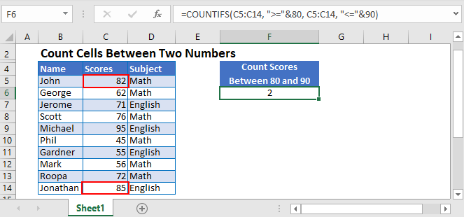
Count Cells Between two Numbers with COUNTIFS
The COUNTIFS Function counts cells that meet multiple conditions. This example will count cells with test scores between 60 and 75:
=COUNTIFS(C3:C12, ">="&60, C3:C12, "<="&75)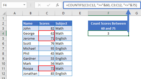
Notice that we must put greater than or equal to and a less than or equal to signs in quotations for the criteria.
The COUNTIFS function also allows you to add further conditions. Using the same example above, let’s say we want to count the number of scores between 60 and 75 in Math.
=COUNTIFS(C3:C12, ">="&60, C3:C12, "<="&75, D3:D12, "Math")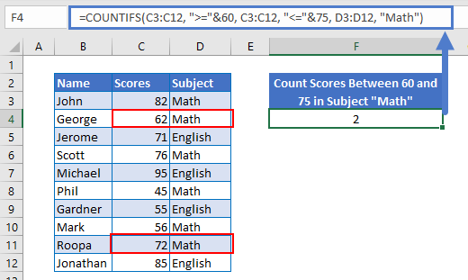
Count Cells Between two Numbers with SUMPRODUCT
You can also use the function SUMPRODUCT to do something similar. The SUMPRODUCT Function is slightly more customizable and is mostly suited for those that are used to Boolean expressions.
Using the same example as above, let’s say we want to count the number of scores between 60 and 75.
=SUMPRODUCT(INT(C3:C12>=60), INT(C3:C12<=75))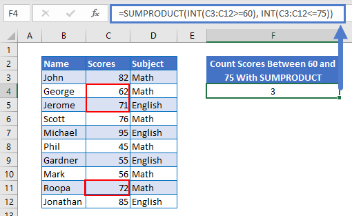
Let’s break this formula down to understand it.
The portion of the formula that says C3:C12>=60 or C3:C12<=75 gives us a TRUE or FALSE result. If the result is TRUE, that means it meets the condition.
The INT Function converts a TRUE value to 1 and a FALSE value to 0.
The SUMPRODUCT function then adds together all the 1 (or TRUE) values which gives us the same result as the COUNTIFS function.
Count cells between two numbers in Google Sheets
These function work the same way in Google Sheets.
=COUNTIFS(C3:C12, ">="&60, C3:C12, "<="&75)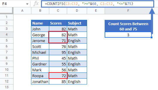
=SUMPRODUCT(INT(C3:C12>=60), INT(C3:C12<=75))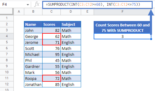
I need a formula to count the number of cells in a range that are between 10 and 10.000:
I have:
=COUNTIF(B2:B292,>10 AND <10.000)
But how do I put the comparison operators in without getting a formula error?
![]()
asked May 2, 2013 at 18:04
![]()
1
If you have Excel 2007 or later use COUNTIFS with an «S» on the end, i.e.
=COUNTIFS(B2:B292,">10",B2:B292,"<10000")
You may need to change commas , to semi-colons ;
In earlier versions of excel use SUMPRODUCT like this
=SUMPRODUCT((B2:B292>10)*(B2:B292<10000))
Note: if you want to include exactly 10 change > to >= — similarly with 10000, change < to <=
answered May 2, 2013 at 18:08
![]()
barry houdinibarry houdini
45.5k8 gold badges63 silver badges80 bronze badges
Example-
For cells containing the values between 21-31, the formula is:
=COUNTIF(M$7:M$83,">21")-COUNTIF(M$7:M$83,">31")
![]()
Shell
6,81010 gold badges39 silver badges70 bronze badges
answered Jun 6, 2014 at 3:13
![]()
=COUNTIFS(H5:H21000,»>=100″, H5:H21000,»<999″)
answered Mar 14, 2018 at 11:44
![]()
1
There has to be someone who it comes down to – to get the clerical work out of the way, fill the administrative shoes, fluff up the white collar. But sitting on the other side of an Excel screen, there’s no need for admin when Excel can be your minion. We’d say that we are counting today but that’s far from the truth; Excel is counting for us the number of cells that carry values between two given numbers.
That promise makes us happy because no one wants to manually count or slave away on any needlessly extensive work on Excel. We’re here to make certain that your Excel life is easy and this is one life you want shortened too. We’re using the COUNTIFS, SUMPRODUCT, COUNT, and FILTER functions in our attempt to count cells whose values match a number range.
We’ll require an example to show you how easy and harmonious this can be and the example is here at the ready.
 1")
Example
See this sample extract we have of some customer orders. Our interest is in column D which enlists the number of items in each order. For now, we are curious about the number of customers who placed an order of between 5 to 10 items.
 2")
No one will stop you if you apply a filter, sort the data according to descending number of ordered items, select the cells and read the Status Bar for the count. But some Excel fairy will be crying bitter tears and she’s more than happy to do the counting for you so we say…..
Let’s get counting!
Using COUNTIFS Function
How about we start by telling Excel to count the cells if they fall between two certain values? That is what the COUNTIFS function will do for us. The ‘S function (see it as a plural of the COUNTIF function) counts the cells that meet the specified conditions.
The two conditions for COUNTIFS will be to find the cells above the lower limit and below the upper limit. The next and final bit will be to count them. Let’s apply the following formula to our case example and see how it works:
=COUNTIFS(D3:D17,"<=10",D3:D17,">=5")
The two conditions we’re passing to the COUNTIFS function are separated by the second comma in the formula. Firstly, the count performed by COUNTIFS should be of cells that carry a value of less than and equal to 10 in the range D3:D17. Then the second condition is applied to the same range but to count cells that are greater than and equal to 5 in value.
This effectively places the counting criteria as greater than, equal to 5 and less than, equal to 10. The COUNTIFS function counts the cells that fulfill these conditions and returns 9.
 3")
This means that there are 9 cells in D3:D17 that have values between 5 to 10. For our case example, that means 9 out of 15 customers placed orders of between 5 to 10 items.
Using SUMPRODUCT Function
Part of understanding the Excel-verse means exploring options and we know another function that can count values between two numbers. This is the SUMPRODUCT function and it multiplies the values in a range with a corresponding range. Then it returns the sum of those values. Used around that concept, SUMPRODUCT makes for a great adding tool to bring together what you need from a range of cells.
Keeping the conditions the same as before, let’s feed it into this formula in a way that will be better accepted by the SUMPRODUCT function:
=SUMPRODUCT((D3:D17>=5)*(D3:D17<=10))
The range given to the SUMPRODUCT function is D3:D17 and the first counting basis is >=5. The second range in the formula is also D3:D17 with the basis for counting as <=10. Both parts in the formula are entered as the same argument (as one array) and have an asterisk in between as the multiplication operator.
Row by row, when every cell in column D is checked to be between 5 to 10, TRUE or FALSE will be returned. But since multiplication requires numbers, the asterisk will force the TRUE and FALSE into 1s and 0s. Then these will be summed by SUMPRODUCT and give us the count again as 9:
 4")
That was one of the many ways to use the SUMPRODUCT function for counting cells. And you can see that we have gotten the desired result from SUMPRODUCT without any Ctrl + Shift + Enter complications of an array formula.
Using COUNT & FILTER Function
We’ll drag your attention back to the start of this tutorial where we were talking about no one stopping you from going the Filter route. Here’s the Excel-seasoned way to do it and it’s going to involve the FILTER function, topped off with the COUNT function – just to make sure it’s not you doing the counting.
The FILTER function filters a range and is like the function version of the Filter feature; you punch in the filtering particulars and the function will filter the data in the range accordingly. The COUNT function counts cells in a range that contains numbers. The formula ahead is an example of how these two functions can work together to count cells with values between two numbers in Excel:
=COUNT(FILTER(D3:D17,(D3:D17>=5)*(D3:D17<=10)))
Beginning with the FILTER function, we’ve supplied the array to be filtered as D3:D17. The logical tests given in the second argument are added with an asterisk (that works like the AND concept) between them and they target column D for values between 5 to 10. Without the COUNT function, the FILTER function will spill its result, returning all the cells matching the given criteria:
=FILTER(D3:D17,{8;7;9;8;9;5;6;8;7})
 5")
Then the COUNT function counts how many cells contain numbers and since there are 9 cells returned by the FILTER function, we get the result as expected:
 6")
By now, you will have learned 3 easy ways of counting cells with values between two numbers with concordant results. For your task, we hope that you can take one of these methods and easily further it if need be. We’ll hurry back with more Excel suggestions that befit or excel the white collar. Are you ready?
This post will guide you how to count cells between two numbers using a formula in Excel 2013/2016. How do I count times between a given range cells based on a condition in Excel. Is there a easy way to count cells between two given numbers in a selected range of cells in Excel.
Table of Contents
- Count Cells between Numbers using COUNTIFS Function
- Count Cells between Numbers using COUNTIF Function
- Related Functions
Count Cells between Numbers using COUNTIFS Function
Assume that you have a list of data in range A1:B6, and you want to count cells between two numbers. In this case, and you can use the COUNTIFS function to achieve the result of counting times between two given numbers in Excel. You should know that the COUNTIFS function will count the number of cells that meet one or more criteria. And the below tutorial will help all levels of Excel users in counting cells between two given numbers in your worksheet.
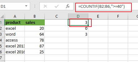
You can use the following formula based on the COUNTIFS function to count cells between 40 and 90.
=COUNTIFS(B2:B6,”>=40″, B2:B6,”<=90″)
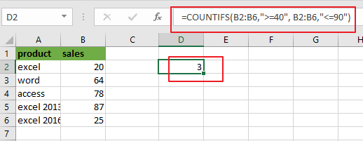
From the above screenshot, and you can see that this formula will count sales number in range B2:B6 that are greater than or equal to 40 and less than or equal to 90. To count cells between two numbers, and you need to provide two criteria in COUNTIFS formula. One is for starting number and one is for the ending number.
Let’s see how this formula works:
The COUNTIFS function can be used to count cells that meet one or more criteria in the given range cells.
This formula has two criteria. It counts the cells in range of cells B2:B6 with values between 40 and 90. The operator “>=” means “greater than or equal to”, and “<=” means “less than or equal to”.
The formula will return the value “3”, which indicates to that there are three cells with values between 40 and 90 in your range of cells.
Count Cells between Numbers using COUNTIF Function
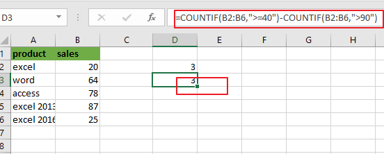
You can also use another function called COUNTIF in an older version of Microsoft Excel to achieve the result of counting cells between two numbers. For the example above you can use the below formula based on the COUNTIF function:
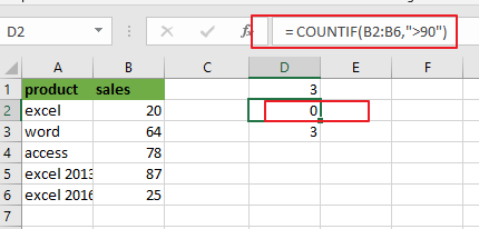
=COUNTIF(B2:B6,”>=40″)-COUNTIF(B2:B6,”>90″)
Let’s see that how this formula works:
The first COUNTIF function will count the number of cells in a range that are greater than or equal to “40”. And the second COUNTIF function will count the number of cells with values that are greater than “90”. And the second number is subtracted from the first result that returned by the first COUNTIF function. Then you should get the number of cells that contain values between 40 and 90.
The First COUNTIF function:
=COUNTIF(B2:B6,”>=40″)
The Second COUNTIF function:
= COUNTIF(B2:B6,”>90″)
- Excel COUNTIF function
The Excel COUNTIF function will count the number of cells in a range that meet a given criteria. This function can be used to count the different kinds of cells with number, date, text values, blank, non-blanks, or containing specific characters.etc.= COUNTIF (range, criteria)… - Excel COUNTIFS function
The Excel COUNTIFS function returns the count of cells in a range that meet one or more criteria. The syntax of the COUNTIFS function is as below:= COUNTIFS(criteria_range1, criteria1, [criteria_range2, criteria2]…)…
While working with Excel, we are able to count cells between two numbers by using the COUNTIFS function. The COUNTIFS function counts the number of cells that meet one or more criteria. This step by step tutorial will assist all levels of Excel users in counting cells between two numbers.
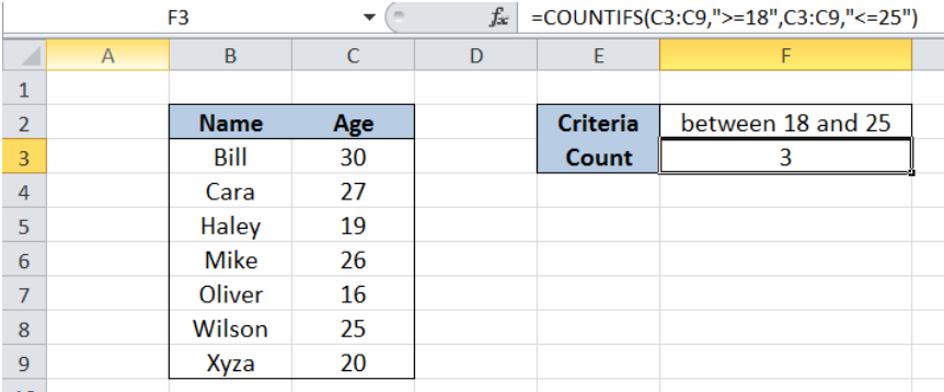 Figure 1. Final result: Count cells between two numbers
Final formula: =COUNTIFS(C3:C9,">=18",C3:C9,"<=25")
Syntax of COUNTIFS Function
=COUNTIFS(criteria_range1, criteria1, [criteria_range2, criteria2]…)
Parameters:
- Criteria_range1: the data range that will be evaluated using the criteria1
- Criteria1: the criteria or condition that determines which cells will be counted
- Criteria_range2 and criteria2 are optional; only applied when there are more than one criteria as specified
Setting up Our Data
Our table contains a list of Names (column B) and Age (column C). Cell F2 contains our criteria which is “between 18 and 25”. The resulting count will be in cell F3.
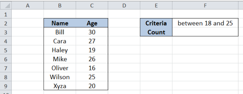 Figure 2. Sample data to count cells between two numbers
Count Cells Between Two Numbers
We want to determine the number of people in the list whose age falls between 18 and 25.
To count the number of cells between two numbers, we will follow these steps:
Step 1. Select cell F3
Step 2. Enter the formula: =COUNTIFS(C3:C9,">=18",C3:C9,"<=25")
Step 3: Press ENTER
The range for our data set is C3:C9. Our formula has two criteria. It counts the cells in column C with values between 18 and 25. The symbol “>=” means “greater than or equal to” while “<=” means “less than or equal to”.
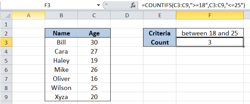 Figure 3. Using the COUNTIFS function to count cells between two numbers
The formula returns the value 3, which corresponds to the three cells with values between 18 and 25 as highlighted below.
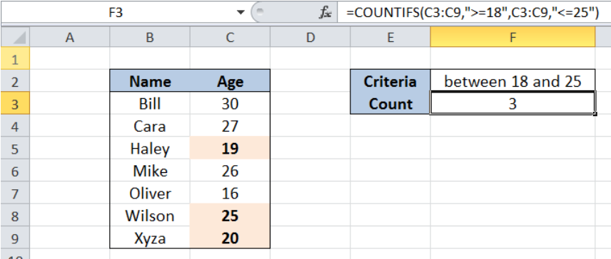 Figure 4. Highlighting the numbers between 18 and 25
Most of the time, the problem you will need to solve will be more complex than a simple application of a formula or function. If you want to save hours of research and frustration, try our live Excelchat service! Our Excel Experts are available 24/7 to answer any Excel question you may have. We guarantee a connection within 30 seconds and a customized solution within 20 minutes.
=COUNTIFS(C8:C12,»>=»&C4,C8:C12,»<=»&C5)
GENERIC FORMULA
=COUNTIFS(range,»>=smallest_num»,range,»<=largest_num»)
ARGUMENTS
range: A range that contains the values from which to count the number of cells that are between two values.
smallest_num: The smallest number from which to count the cells.
largest_num: The largest number from which to count the cells.
GENERIC FORMULA
=COUNTIFS(range,»>=»&smallest_num,range,»<=»&largest_num)
ARGUMENTS
range: A range that contains the values from which to count the number of cells that are between two values.
smallest_num: The smallest number from which to count the cells.
largest_num: The largest number from which to count the cells.
EXPLANATION
This formula uses the COUNTIFS function to count the number of cells that contain values that are between two numbers.
The COUNTIFS function uses two criteria where one states that it must be greater than or equal to the smallest number and the other states that it must be less than or equal to the largest number. The criteria range for both of these criteria is the same, which represents that range that captures the values from which you want to count the cells that fall between the two number. In this example the range from which we are counting the number of cells that fall between the two number is C8 to C12, the smallest number is captured in cell C4 (cell reference) or directly entered into the formula as 50 (hard coded) and the largest number is captured in cell C5 (cell reference) or directly entered into the formula as 100 (hard coded).
Click on either the Hard Coded or Cell Reference button to view the formula that has the smallest and largest number that you want to count between directly entered into the formula or referenced to specific cells.
Last update on August 19 2022 21:50:34 (UTC/GMT +8 hours)
Count cells between numbers
Syntax of used function(s)
COUNTIFS(criteria_range1, criteria1, [criteria_range2, criteria2]…)
Explanation
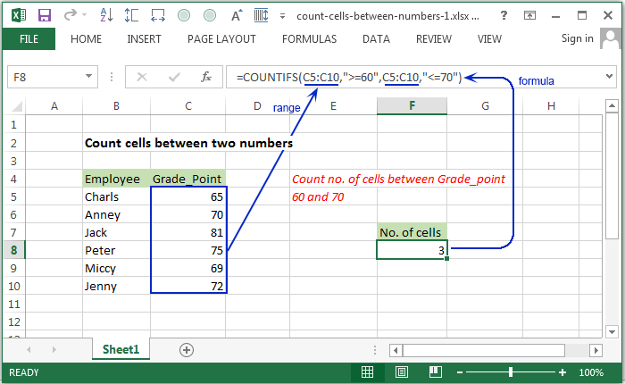
To count the number of cells that contain grade point between two given number, COUNTIFS function can be used.
In the following example, F8 contains this formula:
Formula
=COUNTIFS(C5:C10,">=60",C5:C10,"<=70")
The above fornula contains the grade point of some employees, shown in the range C5:C10.
How this formula works
The COUNTIFS function counts the number of cells that matches one or more criteria.
In this case, two numbers have been provided. The COUNTIFS function will check whether the grade point in the range C5:C10
are in the number range specified in the formula.
Count cells between two numbers using range name
Explanation
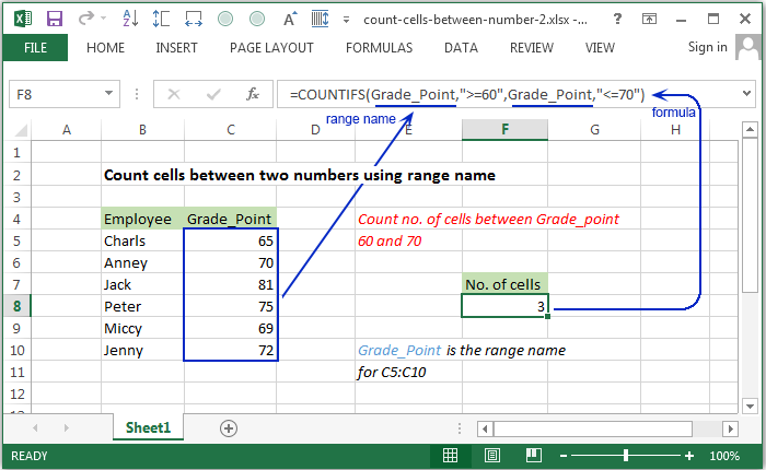
In the following example, F8 contains this formula. A range name «Grade_Point» have been used instead of range C5:C10.
Formula
=COUNTIFS(Grade_Point,">=60",Grade_Point,"<=70")
The above fornula contains the grade point of some employees, shown in the range name «Grade_Point».
How this formula works:
The COUNTIFS function counts cells that matches multiple criteria. Here we use the same range for two criteria.
Each cell in the range must satisfy both criteria in order to be counted.
Grade_Point -> is the range name for the range C5:C10
Count cells between two numbers with criteria
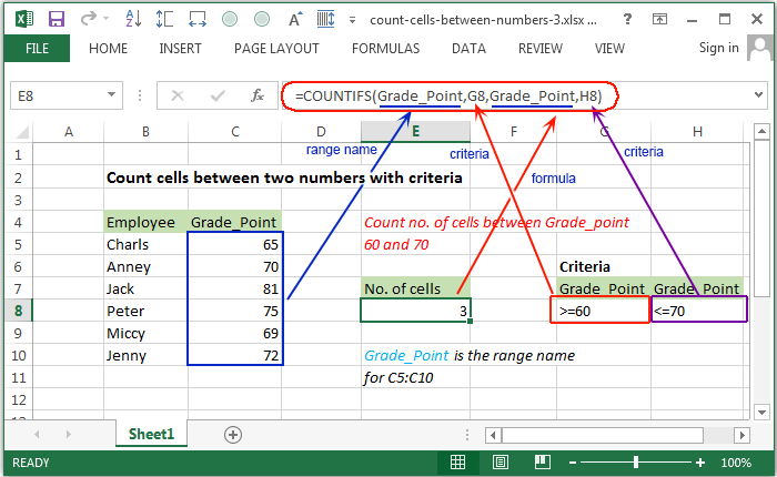
Explanation
In the following example, E8 contains this formula. A range name «Grade_Point» have been used instead of range C5:C10.
And two criteria variable G8 and H8 have been used. G8 contains the value >=60 and H8 contains the value <=70.
Formula
=COUNTIFS(Grade_Point,G8,Grade_Point,H8)
The above formula search each grade point in the range «Grade_Point» between two criteria variables and increase counting
if matches both criteria and produced the result.
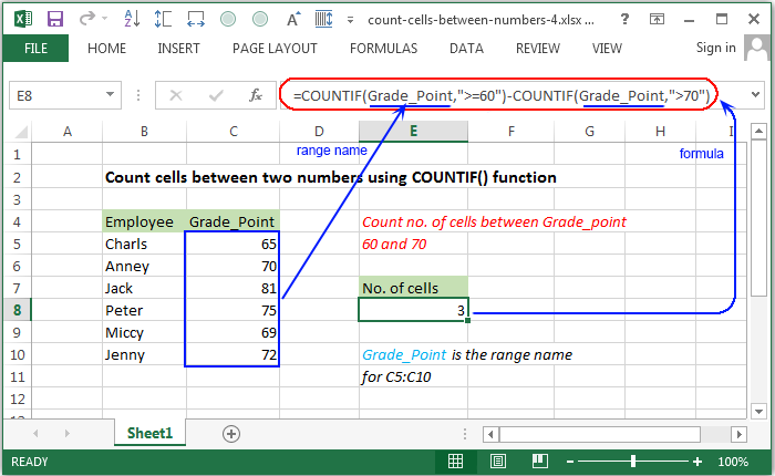
Count cells between two numbers using COUNTIF() function
Syntax of used function(s)
COUNTIF(criteria_range, criteria)
Explanation
In the following example, E8 contains this formula. Two COUNTIF() functions have used in this formula.
A range name «Grade_Point» have used for criteria range and the criterias have used within double inverted quotes.
Formula
=COUNTIF(Grade_Point,">=60")-COUNTIF(Grade_Point,">70")
How this formula works
The first COUNTIF function counts cells that matches the grade point on or above 60 and the second COUNTIF function
matches the grade point above 70. Therefore subtract the result of second criteria from the first criteria.
Count cells using COUNTIF() function with criteria variable
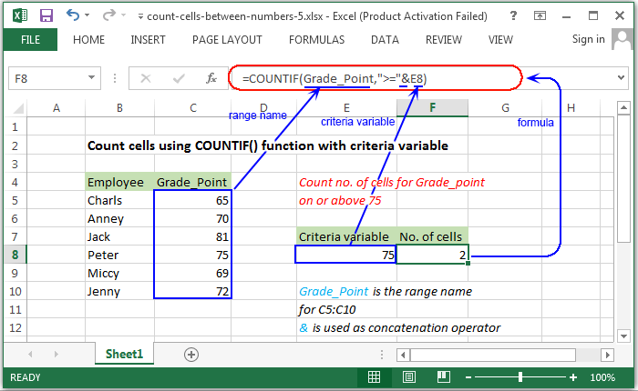
Explanation
In the following example, E8 contains this formula. The COUNTIF() functions have used in this formula.
A range name «Grade_Point» have used for criteria range and a criteria variable have been added with criteria by concatination operator (&).
Formula
=COUNTIF(Grade_Point,">="&E8)
The above example counts number of grade point are on or above the grade point metioned in E8.
Previous: Excel Formulas — Count cells using not equal to operator
Next:
Excel Formulas — Count cells using less than operator