
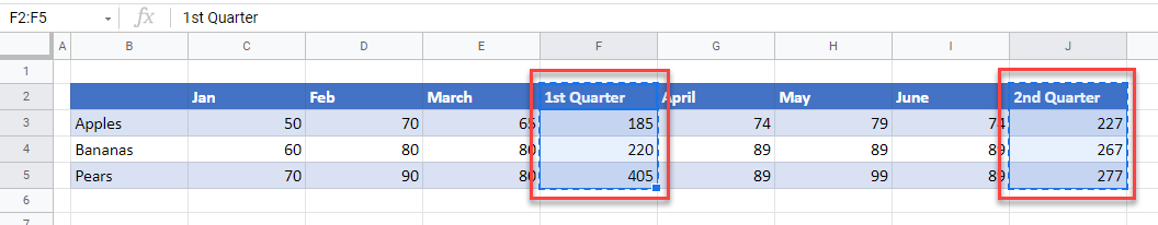
Home / VBA / VBA Copy Range to Another Sheet + Workbook
To copy a cell or a range of cells to another worksheet you need to use the VBA’s “Copy” method. In this method, you need to define the range or the cell using the range object that you wish to copy and then define another worksheet along with the range where you want to paste it.
Copy a Cell or Range to Another Worksheet
Range("A1").Copy Worksheets("Sheet2").Range("A1")- First, define the range or the cell that you want to copy.

- Next, type a dot (.) and select the copy method from the list of properties and methods.

- Here you’ll get an intellisense to define the destination of the cell copied.

- From here, you need to define the worksheet and then the destination range.


Now when you run this code, it will copy cell A1 from the active sheet to the “Sheet2”. There’s one thing that you need to take care that when you copy a cell and paste it to a destination it also pastes the formatting there.
But if you simply want to copy the value from a cell and paste it into the different worksheets, consider the following code.
Worksheets("Sheet2").Range("A1") = Range("A1").ValueThis method doesn’t use the copy method but simply adds value to the destination worksheet using an equal sign and using the value property with the source cell.
Copy Cell from a Different Worksheet
Now let’s say you want to copy a cell from a worksheet that is not active at the time. In this case, you need to define the worksheet with the source cell. Just like the following code.
Worksheets("sheet1").Range("A1").Copy Worksheets("Sheet2").Range("A1")Copy a Range of Cells
Range("A1:A10").Copy Worksheets("Sheet2").Range("A1:A10")
Range("A1:A10").Copy Worksheets("Sheet2").Range("A1")
Copy a Cell to a Worksheet in Another Workbook
When workbooks are open but not saved yet.
Workbooks("Book1").Worksheets("Sheet1").Range("A1").Copy _
Workbooks("Book2").Worksheets("Sheet1").Range("A1")
When workbooks are open and saved.
Workbooks("Book1.xlsx").Worksheets("Sheet1").Range("A1").Copy _
Workbooks("Book2.xlsx").Worksheets("Sheet1").Range("A1")
Copy a Cell to a Worksheet in Another Workbook which is Closed
'to open the workbook that is saved in a folder on your system _
change the path according to the location you have in your _
system
Workbooks.Open "C:UsersDellDesktopmyFile.xlsx"

'copies cell from the book1 workbook and copy and paste _
it to the workbook myFile
Workbooks("Book1").Worksheets("Sheet1").Range("A1").Copy _
Workbooks("myFile").Worksheets("Sheet1").Range("A1")

'close the workbook and after saving
Workbooks("myFile").Close SaveChanges:=True
Related: How to Open a Workbook using VBA in Excel
More Tutorials
- Count Rows using VBA in Excel
- Excel VBA Font (Color, Size, Type, and Bold)
- Excel VBA Hide and Unhide a Column or a Row
- Excel VBA Range – Working with Range and Cells in VBA
- Apply Borders on a Cell using VBA in Excel
- Find Last Row, Column, and Cell using VBA in Excel
- Insert a Row using VBA in Excel
- Merge Cells in Excel using a VBA Code
- Select a Range/Cell using VBA in Excel
- SELECT ALL the Cells in a Worksheet using a VBA Code
- ActiveCell in VBA in Excel
- Special Cells Method in VBA in Excel
- UsedRange Property in VBA in Excel
- VBA AutoFit (Rows, Column, or the Entire Worksheet)
- VBA ClearContents (from a Cell, Range, or Entire Worksheet)
- VBA Enter Value in a Cell (Set, Get and Change)
- VBA Insert Column (Single and Multiple)
- VBA Named Range | (Static + from Selection + Dynamic)
- VBA Range Offset
- VBA Sort Range | (Descending, Multiple Columns, Sort Orientation
- VBA Wrap Text (Cell, Range, and Entire Worksheet)
- VBA Check IF a Cell is Empty + Multiple Cells
⇠ Back to What is VBA in Excel
Helpful Links – Developer Tab – Visual Basic Editor – Run a Macro – Personal Macro Workbook – Excel Macro Recorder – VBA Interview Questions – VBA Codes

This Excel tutorial explains how to copy a range of cells from one location to another in Excel 2016 (with screenshots and step-by-step instructions).
If you want to follow along with this tutorial, download the example spreadsheet.
Download Example
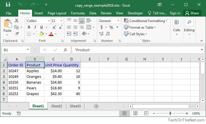
Question: In Microsoft Excel 2016, how do I copy a range of cells along with its formatting to a different location in my spreadsheet?
Answer: By default when you copy and paste and range of cells, it will copy the data as well as formatting such as font, number format, borders, background color, etc.
To copy a range, select the first cell in your range. You will see the cell become active with a black box around it. In this example, we’ve selected cell B1.
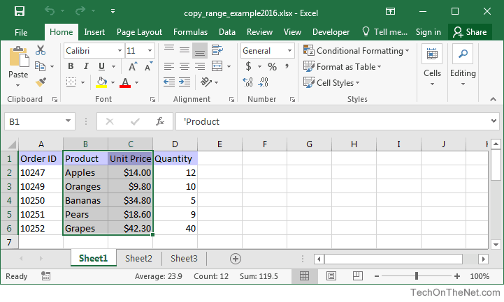
Next, hold down the SHIFT key and click on the last cell in the range. In this example, we have clicked on cell C6. You should see the entire range of cells become highlighted.
TIP: If you want to select an entire column, click on the column letter. If you want to select an entire row, click on the row number.
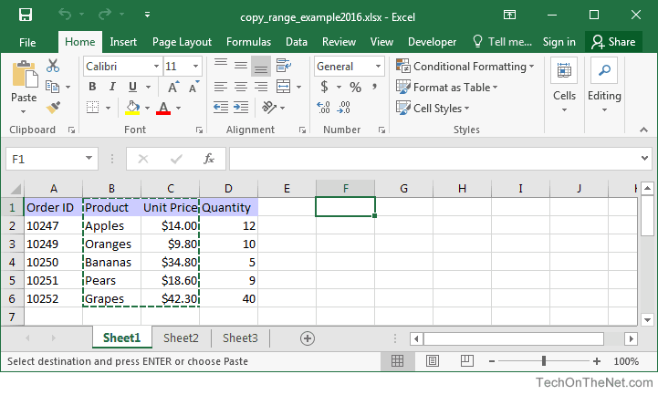
Now to copy the cells, press CTRL + C. You will see a dotted border appear around the range of cells indicating that the cells are in the clipboard and ready to be pasted to another location in your spreadsheet.
Now you will need to select your destination. To do this, select the starting cell where you would like to paste the range. In this example, we have selected cell F1.
To paste the range of cells, press CTRL + V.
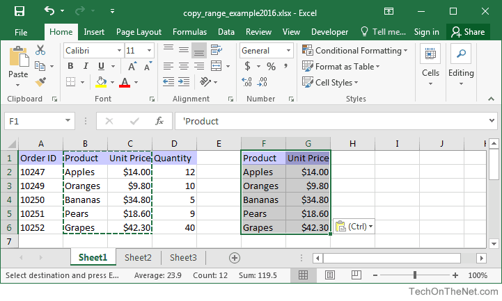
Now you should see the pasted range in the new location in your spreadsheet. In this example, F1:G6 now contains a copy of the data and formatting from the range B1:C6.
Notice that your selected range (B1:C6) still has a dotted border which means that the range is still in your clipboard and you can paste it again to another location in your spreadsheet. When you are done copying and pasting the range, you can press the Escape key. This will clear the clipboard and the range will no longer be highlighted with a dotted border around it.
Вырезание, перемещение, копирование и вставка ячеек (диапазонов) в VBA Excel. Методы Cut, Copy и PasteSpecial объекта Range, метод Paste объекта Worksheet.
Метод Range.Cut
Range.Cut – это метод, который вырезает объект Range (диапазон ячеек) в буфер обмена или перемещает его в указанное место на рабочем листе.
Синтаксис
Параметры
| Параметры | Описание |
|---|---|
| Destination | Необязательный параметр. Диапазон ячеек рабочего листа, в который будет вставлен (перемещен) вырезанный объект Range (достаточно указать верхнюю левую ячейку диапазона). Если этот параметр опущен, объект вырезается в буфер обмена. |
Для вставки на рабочий лист диапазона ячеек, вырезанного в буфер обмена методом Range.Cut, следует использовать метод Worksheet.Paste.
Метод Range.Copy
Range.Copy – это метод, который копирует объект Range (диапазон ячеек) в буфер обмена или в указанное место на рабочем листе.
Синтаксис
Параметры
| Параметры | Описание |
|---|---|
| Destination | Необязательный параметр. Диапазон ячеек рабочего листа, в который будет вставлен скопированный объект Range (достаточно указать верхнюю левую ячейку диапазона). Если этот параметр опущен, объект копируется в буфер обмена. |
Метод Worksheet.Paste
Worksheet.Paste – это метод, который вставляет содержимое буфера обмена на рабочий лист.
Синтаксис
|
Worksheet.Paste (Destination, Link) |
Метод Worksheet.Paste работает как с диапазонами ячеек, вырезанными в буфер обмена методом Range.Cut, так и скопированными в буфер обмена методом Range.Copy.
Параметры
| Параметры | Описание |
|---|---|
| Destination | Необязательный параметр. Диапазон (ячейка), указывающий место вставки содержимого буфера обмена. Если этот параметр не указан, используется текущий выделенный объект. |
| Link | Необязательный параметр. Булево значение, которое указывает, устанавливать ли ссылку на источник вставленных данных: True – устанавливать, False – не устанавливать (значение по умолчанию). |
В выражении с методом Worksheet.Paste можно указать только один из параметров: или Destination, или Link.
Для вставки из буфера обмена отдельных компонентов скопированных ячеек (значения, форматы, примечания и т.д.), а также для проведения транспонирования и вычислений, используйте метод Range.PasteSpecial (специальная вставка).
Примеры
Вырезание и вставка диапазона одной строкой (перемещение):
|
Range(«A1:C3»).Cut Range(«E1») |
Вырезание ячеек в буфер обмена и вставка методом ActiveSheet.Paste:
|
Range(«A1:C3»).Cut ActiveSheet.Paste Range(«E1») |
Копирование и вставка диапазона одной строкой:
|
Range(«A18:C20»).Copy Range(«E18») |
Копирование ячеек в буфер обмена и вставка методом ActiveSheet.Paste:
|
Range(«A18:C20»).Copy ActiveSheet.Paste Range(«E18») |
Копирование одной ячейки и вставка ее данных во все ячейки заданного диапазона:
|
Range(«A1»).Copy Range(«B1:D10») |
Bottom line: Learn 3 different ways to copy and paste cells or ranges in Excel with VBA Macros. This is a 3-part video series and you can also download the file that contains the code.
Skill level: Beginner
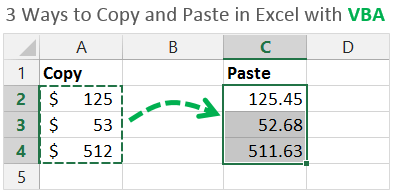
Copy & Paste: The Most Common Excel Action
Copy and paste is probably one of the most common actions you take in Excel. It’s also one of the most common tasks we automate when writing macros.
There are a few different ways to accomplish this task, and the macro recorder doesn’t always give you the most efficient VBA code.
In the following three videos I explain:
- The most efficient method for a simple copy and paste in VBA.
- The easiest way to paste values.
- How to use the PasteSpecial method for other paste types.
You can download the file I use in these videos below. The code is also available at the bottom of the page.
Video #1: The Simple Copy Paste Method
You can watch the playlist that includes all 3 videos at the top of this page.
Video #2: An Easy Way to Paste Values
Video #3: The PasteSpecial Method Explained
VBA Code for the Copy & Paste Methods
Download the workbook that contains the code.
'3 Methods to Copy & Paste with VBA
'Source: https://www.excelcampus.com/vba/copy-paste-cells-vba-macros/
'Author: Jon Acampora

Sub Range_Copy_Examples()
'Use the Range.Copy method for a simple copy/paste

    'The Range.Copy Method - Copy & Paste with 1 line
    Range("A1").Copy Range("C1")
    Range("A1:A3").Copy Range("D1:D3")
    Range("A1:A3").Copy Range("D1")

    'Range.Copy to other worksheets
    Worksheets("Sheet1").Range("A1").Copy Worksheets("Sheet2").Range("A1")

    'Range.Copy to other workbooks
    Workbooks("Book1.xlsx").Worksheets("Sheet1").Range("A1").Copy _
        Workbooks("Book2.xlsx").Worksheets("Sheet1").Range("A1")

End Sub


Sub Paste_Values_Examples()
'Set the cells' values equal to another to paste values

    'Set a cell's value equal to another cell's value
    Range("C1").Value = Range("A1").Value
    Range("D1:D3").Value = Range("A1:A3").Value

    'Set values between worksheets
    Worksheets("Sheet2").Range("A1").Value = Worksheets("Sheet1").Range("A1").Value

    'Set values between workbooks
    Workbooks("Book2.xlsx").Worksheets("Sheet1").Range("A1").Value = _
        Workbooks("Book1.xlsx").Worksheets("Sheet1").Range("A1").Value

End Sub


Sub PasteSpecial_Examples()
'Use the Range.PasteSpecial method for other paste types

    'Copy and PasteSpecial a Range
    Range("A1").Copy
    Range("A3").PasteSpecial Paste:=xlPasteFormats

    'Copy and PasteSpecial a between worksheets
    Worksheets("Sheet1").Range("A2").Copy
    Worksheets("Sheet2").Range("A2").PasteSpecial Paste:=xlPasteFormulas

    'Copy and PasteSpecial between workbooks
    Workbooks("Book1.xlsx").Worksheets("Sheet1").Range("A1").Copy
    Workbooks("Book2.xlsx").Worksheets("Sheet1").Range("A1").PasteSpecial Paste:=xlPasteFormats

    'Disable marching ants around copied range
    Application.CutCopyMode = False

End Sub
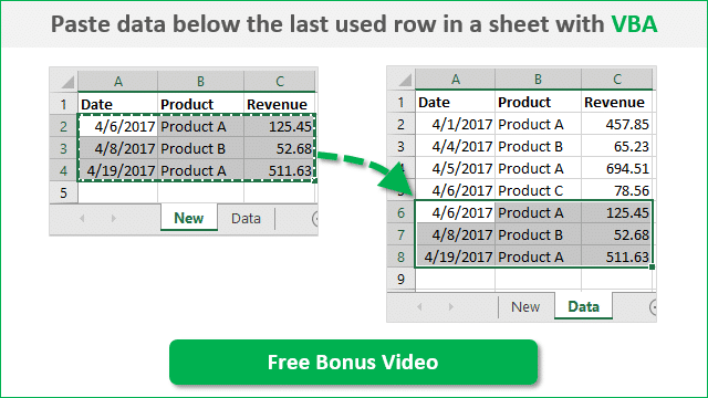
Paste Data Below the Last Used Row
One of the most common questions I get about copying and pasting with VBA is, how do I paste to the bottom of a range that is constantly changing? I first want to find the last row of data, then copy & paste below it.
To answer this question, I created a free training video on how to paste data below the last used row in a sheet with VBA. Can I send you the video? Please click the image below to get the video.
Free Training on Macros & VBA
The 3 videos above are from my VBA Pro Course. If you want to learn more about macros and VBA then checkout my free 3-part video training series.
I will also send you info on the VBA Pro Course, that will take you from beginner to expert. Click the link below to get instant access.
Free Training on Macros & VBA
Please leave a comment below with any questions. Thanks!
I’m looking for a way to copy a range of cells, but to only copy the cells that contain a value.
In my excel sheet I have data running from A1-A18, B is empty and C1-C2. Now I would like to copy all the cells that contain a value.
 With Range("A1")
     Range(.Cells(1, 1), .End(xlDown).Cells(50, 3)).Copy
 End With
This will copy everything from A1-C50, but I only want A1-A18 and C1-C2 to be copied seen as though these contain data. But it needs to be formed in a way that once I have data in B or my range extends, that these get copied too.
'So the range could be 5000 and it only selects the data with a value.
With Range("A1")
Range(.Cells(1, 1), .End(xlDown).Cells(5000, 3)).Copy
End With
Thanks!
Thanks to Jean, Current code:
Sub test()

Dim i As Integer
Sheets("Sheet1").Select
i = 1

With Range("A1")
   If .Cells(1, 1).Value = "" Then
   Else
     Range(.Cells(1, 1), .End(xlDown)).Copy Destination:=Sheets("Sheet2").Range("A" & i)
     x = x + 1
   End If
End With

Sheets("Sheet1").Select

x = 1
With Range("B1")
' Column B may be empty. If so, xlDown will return cell C65536
' and whole empty column will be copied... prevent this.
    If .Cells(1, 1).Value = "" Then
       'Nothing in this column.
       'Do nothing.
    Else
       Range(.Cells(1, 1), .End(xlDown)).Copy Destination:=Sheets("Sheet2").Range("B" & i)
       x = x + 1
    End If
End With

Sheets("Sheet1").Select

x = 1
With Range("C1")
    If .Cells(1, 1).Value = "" Then
    Else
        Range(.Cells(1, 1), .End(xlDown)).Copy Destination:=Sheets("Sheet2").Range("C" & i)
        x = x + 1
    End If
End With

End Sub
A1 — A5 contains data, A6 is blanc, A7 contains data. It stops at A6 and heads over to column B, and continues in the same way.
Copying and Pasting a cell or a range of cells is one of the most common tasks users do in Excel.
A proper understanding of how to copy-paste multiple cells (that are adjacent or non-adjacent) would really help you be a lot more efficient while working with Microsoft Excel.
In this tutorial, I will show you different scenarios where you can copy and paste multiple cells in Excel.
If you have been using Excel for some time now, I’m quite sure you would know some of these already, but there’s a good chance you’d end up learning something new.
So let’s get started!
Copy and Paste Multiple Adjacent Cells
Let’s start with the easy scenario.
Suppose you have a range of cells (that are adjacent) as shown below and you want to copy it to some other location in the same worksheet or some other worksheet/workbook.

Below are the steps to do this:
- Select the range of cells that you want to copy

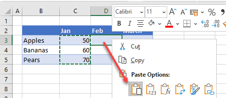
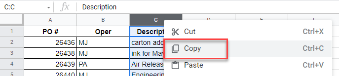
- Right-click on the selection
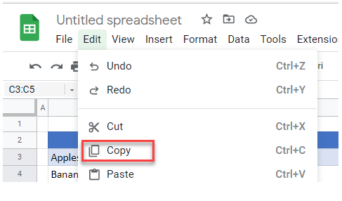
- Click on Copy

- Right-click on the destination cell (E1 in this example)
- Click on the Paste icon
The above steps would copy all the cells in the selected range and paste them into the destination range.

In case you already have something in the destination range, it would be overwritten.
Excel also gives you the flexibility to choose what you want to paste. For example, you can choose to only copy and paste the values, or the formatting, or the formulas, etc.
These options are available to you when you right-click on the destination cell (the icons below the paste special option).
Or you can click on the Paste Special option and then choose what you want to paste using the options in the dialog box.
Useful Keyboard Shortcuts for Copy Paste
In case you prefer using the keyboard while working with Excel, you can use the below shortcut:
- Control + C (Windows) or Command + C (Mac) – to copy range of cells
- Control + V (Windows) or Command + V (Mac) – to paste in the destination cells
And below are some advanced copy-paste shortcuts (using the paste special dialog box).
To use this, first copy the cells, then select the destination cell, and then use the below keyboard shortcuts.
- To paste only the Values – Control + E + S + V + Enter
- To paste only the Formulas – Control + E + S + F + Enter
- To paste only the Formatting – Control + E + S + T + Enter
- To paste only the Column Width – Control + E + S + W + Enter
- To paste only the Comments and notes – Control + E + S + C + Enter
In case you’re using Mac, use Command instead of Control.
Also read: How to Cut a Cell Value in Excel (Keyboard Shortcuts)
Mouse Shortcut for Copy Paste
If you prefer using the mouse instead of the keyboard shortcuts, here is another way you can quickly copy and paste multiple cells in Excel.
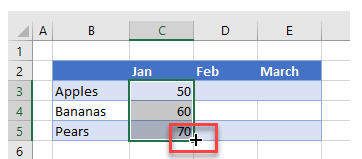
- Select the cells that you want to copy
- Hold the Control key
- Place the mouse cursor at the edge of the selection (you will notice that the cursor changes into an arrow with a plus sign)
- Left-click and then drag the selection where you want the cells to be pasted

This method is also quite fast but is only useful in case you want to copy and paste the range of cells in the same worksheet somewhere nearby.
If the destination cell is a little far off, you’re better off using the keyboard shortcuts.
Copy and Paste Multiple Non-Adjacent Cells
Copy-pasting multiple cells that are nonadjacent is a bit tricky.
If you select multiple cells that are not adjacent to each other, and you copy these cells, you’ll see a prompt as shown below.

This is Excel’s way of telling you that you cannot copy multiple cells that are non-adjacent.
Unfortunately, there’s nothing that you can do about it.
There’s no hack or a workaround, and if you want to copy and paste these nonadjacent cells, you will have to do this one by one.
But there are a few scenarios where you can actually copy and paste non-adjacent cells in Excel.
Let’s have a look at these.
Copy and Paste Multiple Non-Adjacent Cells (that are in the same row/column)
While you can not copy non-adjacent cells in different rows and columns, if you have non-adjacent cells in the same row or column, Excel allows you to copy these.
For example, you can copy cells in the same row (even if these are non-adjacent). Just select the cells and then use Control + C (or Command + C for Mac). You will see the outline (the dancing ants outline).

Once you have copied these cells, go to the destination cell and paste these (Control + V or Command + V)
Excel will paste all the copied cells in the destination cell but make these adjacents.
Similarly, you can select multiple nonadjacent cells in one column, copy them, and then paste it into the destination cells.
Copy and Paste Multiple Non-Adjacent Rows/Columns (but adjacent cells)
Another thing Excel allows is to select non-adjacent rows or non-adjacent columns and then copy them.

Now when you paste these in the destination cell, these would be pasted as adjacent rows or columns.

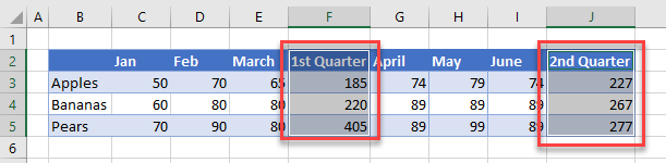
Below is an example where I copied multiple non-adjacent rows from the dataset and pasted these in a different location.
Copy Value From Above in Non-Adjacent Cells
One practical scenario where you may have to copy and paste multiple cells would be when you have gaps in a data set and you want to copy the value from the cell above.
Below I have some dates in column A, and there are some blank cells as well. I want to fill these blank cells with the date in the last filed cell above them.

To do this, I would need to do two things:
- Select all the blank cells
- Copy the date from the above-filled cell and paste it into these blank cells
Let me show you how to do this.
Select All Blank Cells in the Dataset
Below are the steps to select all the blank cells in column A:
- Select the dates in column A, including the blank ones that you want to fill

- Press the F5 key on your keyboard. This will open the Go To dialog box.
- Click the Special button. This will open the Go To Special dialog box.

- In the Go To Special dialog box, select Blanks

- Click OK
The above steps would select all the blank cells in column A.

Now, we want to somehow copy the value in the above field cell in these blank cells. This cannot be done using any copy-paste method so we will have to use a formula (a very simple one).
Fill Blank Cells with Value Above
This part is really easy.
- With the blank cell selected, first hit the equal to key on your keyboard

- Now hit the Up arrow key. This will automatically enter the cell reference of the cell that is above the active cell.

- Hold the Control key and press the Enter key
The above steps would enter the same formula in all the selected blank cells – which is to refer to the cell above it.

While this is a formula, the end result is that you have the blank cells filled with the above-filled date in the data set.
Once you have the desired result, you can convert the formula into values if you want (so that the formula doesn’t update the cells in case you change any value in a cell that is being referenced in the formula).
So these are a couple of methods you can use to copy and paste multiple cells (adjacent and non-adjacent cells) in Excel. I am sure using these methods will help you save tons of time in your day-to-day work.
I hope you found this tutorial useful!
Other Excel tutorials you may also like:
- How to Copy and Paste Column in Excel? 3 Easy Ways!
- How to Copy Excel Table to MS Word (4 Easy Ways)
- How to Copy Conditional Formatting to Another Cell in Excel
- How to Copy and Paste Formulas in Excel without Changing Cell References
- How to Edit Cells in Excel?
This tutorial demonstrates how to copy and paste multiple cells in Excel and Google Sheets.
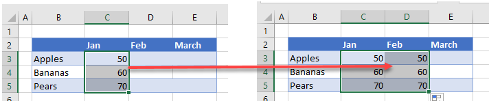
Copy Adjacent Cells
Fill Handle
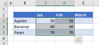
There are several ways that a range of cells can be copied and pasted in Excel. The simplest way to copy multiple or a range of cells across from one column or row to another is use the mouse to drag the values across from one column or row to the next.
- In your worksheet, highlight the cells you wish to copy.
- In the bottom-right corner of your selection, position your mouse so that the mouse pointer changes to a small cross.
- Drag the mouse across to the cells you wish to fill.
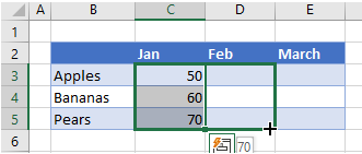
- Release the mouse to copy the information into the blank cells.
‘
This method works well for both copying of cells from column across to an adjacent column on the right, or from a row down to the next row.
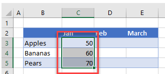
Quick Menu
- In your worksheet, highlight the cells you wish to copy.
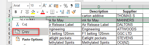
- Right-click on the cells you wish to copy to view the quick menu and click Copy.
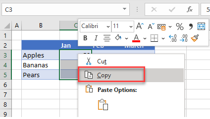
Note that the source cells have small moving lines around them indicating that the information is ready to paste.
- Select the first destination cell and then right-click once again and click Paste.
OR Press the ENTER key on the keyboard to paste the cell data.
Note: You do not have to select the entire destination range where you wish to paste the cell information; you only need to select the first cell.
Copy Nonadjacent Cells
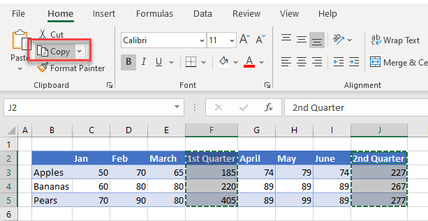
- In your worksheet, highlight the nonadjacent cells you wish to copy by highlighting the first range of cells, and then holding down the CTRL key, highlight the second range of cells.
- Then, in the Ribbon, go to Home > Clipboard > Copy or press CTRL + C on the keyboard. Notice that small little moving lines appear around both selected ranges.
- Select the cell where you wish to paste your data and then, in the Ribbon, go to Home > Clipboard > Paste (or press CTRL + V on the keyboard).
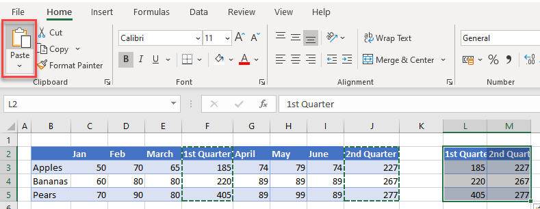
- When you click Paste on the Ribbon, or type CTRL + V on the keyboard, you are left with the small moving lines around your original cells. This is because the information is still on the clipboard and can be pasted as often as you like by using CTRL + V or clicking Paste in the Ribbon. If you wish to exit this mode you can either use ENTER on the keyboard to paste your data, or, if you have already pasted your data, you can press ESC on the keyboard to remove the small moving lines.
Copy Entire Columns and/or Rows
- To copy a column, select the entire column using the column header.
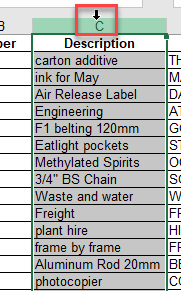
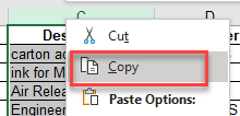
- Right-click to bring up the quick menu and click Copy.
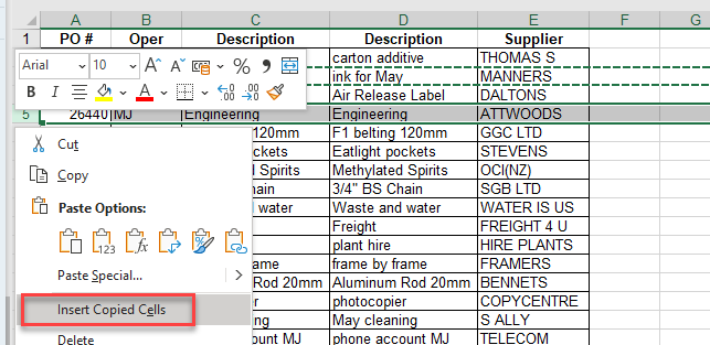
- Select the column where you want to paste the copied cells, and right-click on the column header of the destination column. Click Insert Copied Cells.
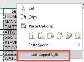
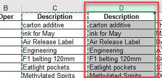
A new column is inserted before the column you selected. This new column will contain the copied cells.
Note: if you have selected a blank column (i.e., no data in any of the cells), you can just press ENTER on the keyboard or choose Paste from the quick menu to paste the copied data into the existing column.
You copy a row in the same way.
- Click in the row header of the row you wish to copy to select the row, and then right-click and click Copy.
- Right-click on the destination row header and to insert a row with the copied data, click Insert Copied Cells, or click Paste to paste the data into an existing row.
Copy Formulas
If you have a cell with a formula in it, and you wish to use that formula in adjacent, or nonadjacent cells, you can copy the formula in the same way as you would copy cells above.
- Select the cell that contains the formula, and then either:
- Right-click, and then click Copy.
OR Press CTRL + C on the keyboard.
OR In the Ribbon, go to Home > Clipboard > Copy.
Small moving lines indicate that the cell has been copied.
- Select the cells where you want to paste the formula.
- Right-click, and then click Paste.
OR Press CTRL + V or ENTER on the keyboard.
OR In the Ribbon, go to Home > Clipboard > Paste.
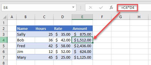
As you look down at the copied formula, you will notice that the formula automatically changes according to the row and column you are copying down or across to.
Note: You can also copy and paste an exact formula so that the row and column information don’t change.
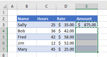
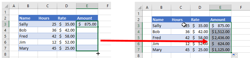
Copy Cell Data or Formula
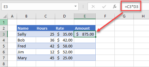
In the picture above, the formatting from cell E3 was pasted into cells E4:E7 along with the formula. The same thing happens when you copy cell data without a formula. To prevent this from happening, use Paste Options to just paste the formulas without the format.
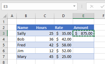
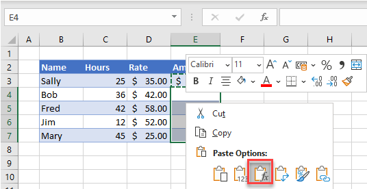
- Copy the cell.
- Then, right-click and choose Paste Options > Paste Formulas.
OR
In the Ribbon, go to Home > Clipboard > Paste > Paste Formulas.
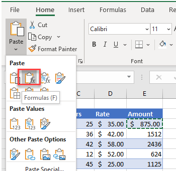
This pastes the formulas into the selected cells without any formatting.
Copy a Formula to Adjacent Cells
You can also drag the formula down to the adjacent cells by using the fill handle.
Notes
- Note that this method will also copy the formatting down to the adjacent cells along with the formula.
- It’s also possible to use Paste Options to paste the formula as text.
Copy-Paste Multiple Cells in Google Sheets
Copying and pasting in Google Sheets works in much the same way as it does in Excel.
- Highlight the cells you wish to copy, and then, on the keyboard press CTRL + C or in the Menu, go to Edit > Copy.
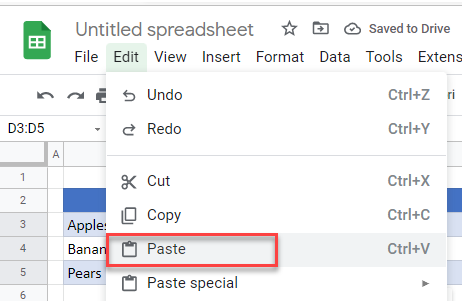
- Select the destination cell and press CTRL + V on the keyboard, or in the Menu, go to Edit > Paste.
You may get a message that you need to install an extension to use Edit > Paste.

You can either dismiss the information message and use CTRL + V to paste the cell data, or you can install the extension into your browser to enable you to use Edit > Paste on the menu.
As with Excel, you can use Paste Special to paste only part of the cell contents: formulas, values, format, etc.
- In the Menu, go to Edit > Paste special and then select the option required.
Adjacent Cells
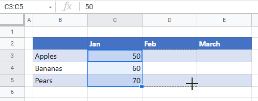
To copy the cell data across to adjacent cells using the mouse, highlight the cells containing the data, and then, drag the mouse pointer across to the desired destination cells.
Nonadjacent Cells
Selecting nonadjacent cell ranges in Google Sheets works the same as in Excel. Select the first range then, holding down the CTRL key, select the second range. Then copy both ranges using CTRL + C or in the Menu, go to Edit > Copy.
Select the destination location and the press CTRL + V or, in the Menu, go to Edit > Paste.
Copy Entire Columns and Rows
- As with Excel, right-click in the header of the column, then click Copy.
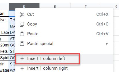
- Right-click in the column header of the destination column. Google will not automatically insert a new column so insert a column first if you do not wish to overwrite the data already in the column. Click Insert 1 column left.
- Right-click in the new column header and click Paste.
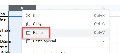
The copied data is pasted into the new column.
Copying an entire row works in the same way; just click the row header instead of the column header!
More Options
For more information on copying and pasting in Excel and Google Sheets, see:
- Copy and Paste Exact Formula
- Copy and Paste Non-Blank Cells (Skip Blanks)
- Copy and Paste Without Borders
- Paste Horizontal Data Vertically
- Rearrange Columns
- Duplicate Rows
- VBA Value Paste & Paste Special
- VBA – Cut, Copy, Paste from a Macro
- VBA Copy / Paste Rows & Columns
- Select Nonadjacent Cells or Columns
- Copy Cell From Another Sheet
") Copy and paste are 2 of the most common Excel operations. Copying and pasting a cell range (usually containing data) is an essential skill you’ll need when working with Excel VBA.
Copy and paste are 2 of the most common Excel operations. Copying and pasting a cell range (usually containing data) is an essential skill you’ll need when working with Excel VBA.
You’ve probably copied and pasted many cell ranges manually. The process itself is quite easy.
Well…
You can also copy and paste cells and ranges of cells when working with Visual Basic for Applications. As you learn in this Excel VBA Tutorial, you can easily copy and paste cell ranges using VBA.
However, for purposes of copying and pasting ranges with Visual Basic for Applications, you have a variety of methods to choose from.
My main objective with this Excel tutorial is to introduce to you the most important VBA methods and properties that you can use for purposes of carrying out these copy and paste activities with Visual Basic for Applications in Excel. In addition to explaining everything you need to know in order to start using these different methods and properties to copy and paste cell ranges, I show you 8 different examples of VBA code that you can easily adjust and use immediately for these purposes.
The following table of contents lists the main topics (and VBA methods) that I cover in this blog post. Use the table of contents to navigate to the topic that interests you at the moment, but make sure to read all sections 😉 .
Let’s start by taking a look at some information that will help you to easily modify the source and destination ranges of the sample macros I provide in the sections below (if you need to).
Scope Of Macro Examples In This Tutorial And How To Modify The Source Or Destination Cells
As you’ve seen in the table of contents above, this Excel tutorial covers several different ways of copying and pasting cells ranges using VBA. Each of these different methods is accompanied by, at least, 1 example of VBA code that you can adjust and use immediately.
All of these macro examples assume that the sample workbook is active and the whole operation takes place on the active workbook. Furthermore, they are designed to copy from a particular source worksheet to another destination worksheet within that sample workbook.
You can easily modify these behaviors by adjusting the way in which the object references are built. You can, for example, copy a cell range to a different worksheet or workbook by qualifying the object reference specifying the destination cell range.
Similar comments apply for purposes of modifying the source and destination cell ranges. More precisely, to (i) copy a different range or (ii) copy to a different destination range, simply modify the range references.
For example, in the VBA code examples that I include throughout this Excel tutorial, the cell range where the source data is located is referred to as follows:
Worksheets("Sample Data").Range("B5:M107")
This reference isn’t a fully qualified object reference. More precisely, it assumes that the copying and pasting operations take place in the active workbook.
The following reference is the equivalent of the above, but is fully qualified:
Workbooks("Book1.xlsm").Worksheets("Sample Data").Range("B5:M107")
This fully qualified reference doesn’t assume that Book1.xlsm is the active workbook. Therefore, the reference works appropriately regardless of which Excel workbook is active.
I explain how to work with object references in detail in The Essential Guide To Excel’s VBA Object Model And Object References. Similarly, I explain how to work with cell ranges in Excel’s VBA Range Object And Range Object References: The Tutorial for Beginners. I suggest you refer to these posts if you feel you need to refresh your knowledge about these topics, or if you’re not familiar with them. They will probably help you to better understand this Excel tutorial and how to modify the sample macros I include here.
You’ll also notice that within the VBA code examples that I include in this Excel tutorial, I always qualify the references up to the level of the worksheet. Strictly speaking, this isn’t always necessary. In fact, when implementing similar code in your VBA macros, you may want to modify the references by, for example:
- Using variables.
- Further simplifying the object references (not qualifying them up to the level of the worksheet).
- Using the With… End With statement.
The reason I’ve decided to keep references qualified up to the level of the worksheet is because the focus of this Excel tutorial is on how to copy and paste using VBA. Not on simplifying references or using variables, which are topics I cover in separate blog posts, such as those I link to above (and which I suggest you take a look at).
The Copy Command In Excel’s Ribbon
Before we go into how to copy a range using Visual Basic for Applications, let’s take a quick look at Excel’s ribbon:
Perhaps one of the most common used buttons in the Ribbon is “Copy”, within the Home tab.

When you think about copying ranges in Excel, you’re probably referring to the action carried out by Excel when you press this button: copying the current active cell or range of cells to the Clipboard.
You may have noticed, however, that the Copy button isn’t just a simple button. It’s actually a split button:
I explain how you can automate the functions of both of these commands in this Excel tutorial. More precisely:
- If you want to work with the regular Copy command, you’ll want to read more about the Range.Copy method, which I explain in the following section.
- If you want to use the Copy as Picture command, you’ll be interested in the Range.CopyPicture method, which I cover below.
Let’s start by taking a look at…
Excel VBA Copy Paste With The Range.Copy Method
The main purpose of the Range.Copy VBA method is to copy a particular range.
When you copy a range of cells manually by, for example, using the “Ctrl + C” keyboard shortcut, the range of cells is copied to the Clipboard. You can use the Range.Copy method to achieve the same thing.
However, the Copy method provides an additional option:
Copying the selected range to another range. You can achieve this by appropriately using the Destination parameter, which I explain in the following section.
In other words, you can use Range.Copy for copying a range to either of the following:
- The Clipboard.
- A certain range.
The Range.Copy VBA Method: Syntax And Parameters
The basic syntax of the Range.Copy method is as follows:
expression.Copy(Destination)
“expression” is the placeholder for the variable representing the Range object that you want to copy.
The only parameter of the Copy VBA method is Destination. This parameter is optional, and allows you to specify the range to which you want to copy the copied range. If you omit the Destination parameter, the copied range is simply copied to the Clipboard.
This means that the appropriate syntax you should use for the Copy method (depending on your purpose) is as follows:
- To copy a Range object to the Clipboard, omit the Destination parameter. In such a case, use the following syntax:
expression.Copy
- To copy the Range object to another (the destination) range, use the Destination parameter to specify the destination range. This means that you should use the following syntax:
expression.Copy(Destination)
Let’s take a look at how you can use the Range.Copy method to copy and paste a range of cells in Excel:
Macro Examples #1 And #2: The VBA Range.Copy Method
This Excel VBA Copy Paste Tutorial is accompanied by an Excel workbook containing the data and macros I use. You can get immediate free access to this workbook by clicking the button below.

For this particular example, I’ve created the following table. This table displays the sales of certain items (A, B, C, D and E) made by 100 different sales managers in terms of units and total Dollar value. The first row (above the main table), displays the unit price for each item. The last column displays the total value of the sales made by each manager.

Macro Example #1: Copy A Cell Range To The Clipboard
First, let’s take a look at how you can copy all of the items within the sample worksheet (table and unit prices) to the Clipboard. The following simple macro (called “Copy_to_Clipboard”) achieves this:

This particular Sub procedure is made out of the following single statement:
Worksheets("Sample Data").Range("B5:M107").Copy
This statement is made up by the following 2 items:
Let’s take a look at this macro in action. Notice how, once I execute the Copy_to_Clipboard macro, the copied range of cells is surrounded by the usual dashed border that indicates that the range is available for pasting.
After executing the macro, I go to another worksheet and paste all manually. As a last step, I autofit the column width to ensure that all the data is visible.

Even though the sample Copy_to_Clipboard macro does what it’s supposed to do and is a good introduction to the Range.Copy method, it isn’t very powerful. It, literally, simply copies the relevant range to the Clipboard. You don’t really need a macro to do only that.
Fortunately, as explained above, the Range.Copy method has a parameter that allows you to specify the destination of the copied range. Let’s use this to improve the power of the sample macro:
Macro Example #2: Copy A Cell Range To A Destination Range
The following sample Sub procedure (named “Copy_to_Range”) takes the basic Copy_to_Clipboard macro used as example #1 above and adds the Destination parameter.

Even though it isn’t the topic of this Excel tutorial, I include an additional statement that uses the Range.AutoFit method.

Let’s take a closer look at each of the lines of code within this sample macro:
Line #1: Worksheets(“Sample Data”).Range(“B5:M107”).Copy
This is, substantially, the sample “Copy_to_Clipboard” macro which I explain in the section above.
More precisely, this particular line uses the Range.Copy method for purposes of copying the range of cells cells B5 and M107 of the worksheet called “Sample Data”.
However, at this point of the tutorial, our focus isn’t in the Copy method itself but rather in the Destination parameter which appears in…
Line #2: Destination:=Worksheets(“Example 2 – Destination”).Range(“B5:M107”)
You use the Destination parameter of the Range.Copy method for purposes of specifying the destination range in which to which the copied range of cells should be copied. In this particular case, the destination range is cells B5 to M107 of the worksheet named “Example 2 – Destination”, as shown in the image below:

As I explain above, you can easily modify this statement for purposes of specifying a different destination. For example, for purposes of specifying a destination range in a different Excel workbook, you just need to qualify the object reference.
Line #3: Worksheets(“Example 2 – Destination”).Columns(“B:M”).AutoFit
As anticipated above, this statement isn’t absolutely necessary for the sample macro to achieve its main purpose of copying the copied range in the destination range. Its purpose is solely to autofit the column width of the destination range.
For these purposes, I use the Range.Autofit method. The syntax of this method is as follows:
expression.AutoFit
In this particular case, “expression” represents a Range object, and must be either (i) a range of 1 or more rows, or (ii) a range of 1 or more columns. In the Copy_to_Range macro example, the Range object is columns B through M of the worksheet titled “Example 2 – Destination”. The following image shows how this range is specified within the VBA code.

The following image shows the results obtained when executing the Copy_to_Range macro. Notice how this worksheet looks substantially the same as the source worksheet displayed above.

If you were to compare the results obtained when copying a range to the Clipboard (example #1) with the results obtained when copying the range to a destination range (example #2), you may conclude that the general rule is that one should always use the Destination parameter of the Copy method.
To a certain extent, this is generally true and some Excel authorities generally discourage using the Clipboard. However, the choice between copying to the Clipboard or copying to a destination range isn’t always so straightforward. Let’s take a look at why this is the case:
The Range.Copy VBA Method: When To Copy To The Clipboard And When To Use The Destination Parameter
In my opinion, if you can achieve your purposes without copying to the Clipboard, you should simply use the Destination parameter of the Range.Copy method.
Using the Destination parameter is, generally, more efficient that copying to the Clipboard and then using the Range.PasteSpecial method or the Worksheet.Paste method (both of which I explain below). Copying to the Clipboard and pasting (with the Range.PasteSpecial or Worksheet.Paste methods) involves 2 steps:
- Copying.
- Pasting.
This 2-step process (usually):
- Increases the procedure’s memory requirements.
- Results in (slightly) less efficient procedures.
I explain this argument further in example #4 below, which introduces the Worksheet.Paste method. The Worksheet.Paste method is one of the VBA methods you’d use for purposes of pasting the data that you’ve copied to the Clipboard with the Range.Copy method.
Avoiding the Clipboard whenever possible may be a good idea to reduce the risks of data loss or leaks of information whenever another application is using the Clipboard at the same time. Some users report unpredictable Clipboard behavior in certain cases.
Considering this arguments, you probably understand why I say that, if you can avoid the Clipboard, you probably should.
However, using the Range.Copy method with the Destination parameter may not be the most appropriate solution always. For purposes of determining when the Destination parameter allows you to achieve the purpose you want, it’s very important that you’re aware of how the Range.Copy method works, particularly what it can (and can’t do). Let’s see an example of what I mean:
If you go back to the screenshots showing the results of executing the sample macros #1 (Copy_to_Clipboard) and #2 (Copy_to_Range), you’ll notice that the end result is that the destination worksheet looks pretty much the same as the source worksheet.
In other words, Excel copies and pastes all (for ex., values, formulas, formats).
In some cases, this is precisely what you want. However:
In other cases, this is precisely what you don’t want. Take a look, for example, at the following Sub procedure:

At first glance, this is the Copy_to_Range macro that I introduce and explain in the section above. Notice, however, that I’ve changed the Destination parameter. More precisely, in this version of the Copy_to_Range macro, the top-left cell of the destination range is cell B1 (instead of B5, as it was originally) of the “Example 2 – Destination” worksheet.

The following GIF shows what happens when I execute this macro. The worksheet shown is the destination “Example 2 – Destination” worksheet, and I’ve enabled iterative calculations (I explain to you below why I did this).

As you can see immediately, there’s something wrong. The total sales for all items are, clearly, inaccurate.

The reason for this is that, in the original table, I used mixed references in order to refer to the unit prices of the items. Notice, for example, the formula used to calculate the total sales of Item A made by Sarah Butler (the first Sales Manager in the table):

These formulas aren’t a problem as long as the destination cells are exactly the same as the source cells. This is the case in both examples #1 and #2 above where, despite the worksheet changing, the destination continues to be cells B5 to M107. That guarantees that the mixed references continue to point to the right cell.
However, once the destination range changes (as in the example above), the original mixed references wreak havoc on the worksheet. Take a look, for example, at the formula used to calculate the total sales of Item B by Sales Manager Walter Perry (second in the table):

The formula doesn’t use the unit price of Item B (which appears in cell F1) to calculate the sales. Instead, it uses cell F5 as a consequence of the mixed references copied from the source worksheet. This results in (i) the wrong result and (ii) a circular reference.
By the way, if you’re downloading the sample workbook that accompanies this Excel tutorial, it will have circular references.
In such (and other similar) cases, you may not want to rely solely on the Range.Copy method with the Destination parameter. In other words: There are cases where you don’t want to copy and paste all the contents of the source cell range. There are, for example, cases where you may want to:
- Copy a cell range containing formulas; and
- Paste values in the destination cell range.
This is precisely what happens in the case of the example above. In such a situation, you may want to paste only the values (no formulas).
For purposes of controlling what is copied in a particular destination range when working with VBA, you must understand the Range.PasteSpecial method. Let’s take a look at it:
Excel VBA Copy Paste With The Range.PasteSpecial Method
Usually, whenever you want to control what Excel copies in a particular destination range, you rely on the Paste Special options. You can access these options, for example, through the Paste Special dialog box.

When working with Visual Basic for Applications, you usually rely on the Range.PasteSpecial method for purposes of controlling what is copied in the destination range.
Generally speaking, the Range.PasteSpecial method allows you to paste a particular Range object from the Clipboard into the relevant destination range. This, by itself, isn’t particularly exciting.
The power of the Range.PasteSpecial method comes from its parameters, and the ways in which they allow you to further determine the way in which Excel carries out the pasting. Therefore, let’s take a look at…
The Range.PasteSpecial VBA Method: Syntax And Parameters
The basic syntax of the Range.PasteSpecial method is as follows:
expression.PasteSpecial(Paste, Operation, SkipBlanks, Transpose)
“expression” represents a Range object. The PasteSpecial method has 4 optional parameters:
- Parameter #1: Paste.
- Parameter #2: Operation.
- Parameter #3: SkipBlanks.
- Parameter #4: Transpose.
Notice how each of these parameters roughly mimics most of the different sections and options of the Paste Special dialog box shown above. The main exception to this general rule is the Paste Link button.

I explain how you can paste a link below.
For the moment, let’s take a closer look at each of these parameters:
Parameter #1: Paste
The Paste parameter of the PasteSpecial method allows you to specify what is actually pasted. This parameter is the one that, for example, allows you specify that only the values (or the formulas) should be pasted in the destination range.
This is, roughly, the equivalent of the Paste section in the Paste Special dialog box shown below:

The Paste parameter can take any of 12 values that are specified in the XlPasteType enumeration:
Parameter #2: Operation
The Operation parameter of the Range.PasteSpecial method allows you to specify whether a mathematical operation is carried out with the destination cells. This parameter is roughly the equivalent of the Operation section of the Paste Special dialog box.

The Operation parameter can take any of the following values from the XlPasteSpecialOperation enumeration:
Parameter #3: SkipBlanks
You can use the SkipBlanks parameter of the Range.PasteSpecial method to specify whether the blank cells in the copied range should be (or not) pasted in the destination range.

SkipBlanks can be set to True or False, as follows:
- If SkipBlanks is True, the blank cells within the copied range aren’t pasted in the destination range.
- If SkipBlanks is False, those blank cells are pasted.
False is the default value of the SkipBlanks parameter. If you omit SkipBlanks, the blank cells are pasted in the destination range.
Parameter #4: Transpose
The Transpose parameter of the Range.PasteSpecial VBA method allows you to specify whether the rows and columns of the copied range should be transposed (their places exchanged) when pasting.

You can set Transpose to either True or False. The consequences are as follows:
- If Transpose is True, rows and columns are transposed when pasting.
- If Transpose is False, Excel doesn’t transpose anything.
The default value of the Transpose parameter is False. Therefore, if you omit it, Excel doesn’t transpose the rows and columns of the copied range.
Macro Example #3: Copy And Paste Special
Let’s go back once more to the sample macros and see how we can use the Range.PasteSpecial method to copy and paste the sample data.
The following sample Sub procedure, called “Copy_PasteSpecial” shows 1 of the many ways in which you can do this:

When using the Range.Copy method to copy to the Clipboard (as in the case above) you can end the macro with the statement “Application.CutCopyMode = False”, which I explain in more detail towards the end of this blog post. This particular statement cancels Cut or Copy mode and removes the moving border.
Let’s take a look at each of the lines of code to understand how this macro achieves its purpose:
Line #1: Worksheets(“Sample Data”).Range(“B5:M107”).Copy
This statement appears in both of the previous examples.
As explained in those previous sections, its purpose is to copy the range between cells B5 and M107 of the worksheet named “Sample Data” to the Clipboard.
Lines #2 Through #6 Worksheets(“Example 3 – PasteSpecial”).Range(“B5”).PasteSpecial Paste:=xlPasteValuesAndNumberFormats, Operation:=xlPasteSpecialOperationNone, SkipBlanks:=False, Transpose:=True
These lines of code make reference to the Range.PasteSpecial method that I explain in the previous section. In order to take a closer look at it, let’s break down this statement into the following 6 items:

And let’s take a look at each of the items separately:
- Item #1: “Worksheets(“Example 3 – PasteSpecial”).Range(“B5″)”.
- This is a Range object. Within the basic syntax of the PasteSpecial method that I introduce above, this item is the “expression”.
- This range is the destination range, where the contents of the Clipboard are pasted. In this particular case, the range is identified by its worksheet (“Example 3 – PasteSpecial” of the active workbook) and the upper-left cell of the cell range (B5).
- To paste the items that you have in the Clipboard in a different workbook, simply qualify this reference as required and explained above.
- Item #2: “PasteSpecial”.
- This item simply makes reference to the Range.PasteSpecial method.
- Item #3: “Paste:=xlPasteValuesAndNumberFormats”.
- This is the Paste parameter of the PasteSpecial method. In this particular case, the argument is set to equal xlPasteValuesAndNumberFormats. The consequence of this, as explained above, is that only values and number formats are pasted. Other items, such as formulas and borders, aren’t pasted in the destination range.
- Item #4: “Operation:=xlPasteSpecialOperationNone”.
- The line sets the Operation parameter of the Range.PasteSpecial method to be equal to xlPasteSpecialOperationNone. As I mention above, this means that Excel carries out no calculation when pasting the contents of the Clipboard.
- Item #5: “SkipBlanks:=False”.
- This line confirms that the value of the SkipBlanks parameter is False (which is its default value anyway). Therefore, if there were blank cells in the range held by the Clipboard, they would be pasted in the destination.
- Item #6: “Transpose:=True”.
- The final parameter of the Range.PasteSpecial method (Transpose) is set to True by this line. As a consequence of this, rows and columns are transposed upon being pasted.
The purpose of this code example is just to show you some of the possibilities that you have when working with the Range.PasteSpecial VBA method. It doesn’t mean it’s how I would arrange the data it in real life. For example, if I were implementing a similar macro for copying similarly organized data, I wouldn’t transpose the rows and columns (you can see how the transposing looks like in this case further below).
In any case, since the code includes all of the parameters of the Range.PasteSpecial method, and I explain all of those parameters above, you shouldn’t have much problem making any adjustments.
Line #7: Worksheets(“Example 3 – PasteSpecial”).Columns(“B:CZ”).AutoFit
This line is substantially the same as the last line of code within example #2 above (Copy_to_Range). Its purpose is exactly the same:
This line uses the Range.AutoFit method for purposes of autofitting the column width.
The only difference between this statement and that in example #2 above is the column range to which it is applied. In example #2 (Copy_to_Range) above, the autofitted columns are B to M (Range(“B5:M107”)). In this example #3 (Copy_PasteSpecial), the relevant columns are B to CZ (Columns(“B:CZ”)).
The reason why I make this adjustment is the layout of the data and, more precisely, the fact that the Copy_PasteSpecial macro transposes the rows and columns. This results in the table extending further horizontally.
The following screenshot shows the results of executing the Copy_PasteSpecial macro. Notice, among others, how (i) no borders have been pasted (a consequence of setting the Paste parameter to xlPasteValuesAndNumberFormats), and (ii) the rows and columns are transposed (a consequence of setting Transpose to equal True).

If you only need to copy values (the equivalent of setting the Paste parameter to xlPasteValues) or formulas (the equivalent of setting the Paste parameter to xlPasteFormulas), you may prefer to set the values or the formulas of the destination cells to be equal to that of the source cells instead of using the Range.Copy and Range.PasteSpecial methods. I explain how you can do this (alongside an example) below.
As you can see, you can use the PasteSpecial method to replicate all of the options that appear in the Paste Special dialog box, except for the Paste Link button that appears on the lower left corner of the dialog.

Let’s take a look at a VBA method you can use for these purposes:
Excel VBA Copy Paste With The Worksheet.Paste Method
The Worksheet.Paste VBA method (Excel VBA has no Range.Paste method) is, to a certain extent, very similar to the Range.PasteSpecial method that I explain in the previous section. The main purpose of the Paste method is to paste the contents contained by the Clipboard on the relevant worksheet.
However, as the following section makes clear, there are some important differences between both methods, both in terms of syntax and functionality. Let’s take a look at this:
Worksheet.Paste VBA Method: Syntax And Parameters
The basic syntax of the Worksheet.Paste method is:
expression.Paste(Destination, Link)
The first difference between this method and the others that I explain in previous sections is that, in this particular case, “expression” stands for a Worksheet object. In other cases we’ve seen in this Excel tutorial (such as the Range.PasteSpecial method), “expression” is a variable representing a Range object.
The Paste method has the following 2 optional parameters. They have some slightly particular conditions which differ from what we’ve seen previously in this same blog post.
- Destination: Destination is a Range object where the contents of the Clipboard are to be pasted.
- Since the Destination parameter is optional, you can omit it. If you omit Destination, Excel pastes the contents of the Clipboard in the current selection. Therefore, if you omit the argument, you must select the destination range before using the Worksheet.Paste method.
- You can only use the Destination argument if 2 conditions are met: (i) the contents of the Clipboard can be pasted into a range, and (ii) you’re not using the Link parameter.
- Link: You use the Link parameter for purposes of establishing a link to the source of the pasted data. To do this, you set the value to True. The default value of the parameter is False, meaning that no link to the source data is established.
- If you’re using the Destination parameter when working with the Worksheet.Paste method, you can’t use the Link parameter. Macro example #5 below shows how one way in which you can specify the destination for pasting links.
Let’s take a look at 2 examples that show the Worksheet.Paste method working in practice:
Macro Example #4: Copy And Paste
The following sample macro (named “Copy_Paste”) works with exactly the same data as the previous examples. It shows how you can use the Worksheet.Paste method for purposes of copying and pasting data.

Just as with the previous example macro #3, since this particular macro uses the Clipboard, you can add the statement “Application.CutCopyMode = False” at the end of the macro for purposes of cancelling the Cut or Copy mode. I explain this statement in more detail below.
Let’s take a look at each of the lines of code to understand how this sample macro proceeds:
Line #1: Worksheets(“Sample Data”).Range(“B5:M107”).Copy
This statement is the same as the first statement of all the other sample macros that I’ve introduced in this blog post. I explain its different items the first time is used.
Its purpose is to copy the contents within cells B5 to M107 of the “Sample Data” worksheet to the Clipboard.
Lines #2 And #3: Worksheets(“Example 4 – Paste”).Paste Destination:=Worksheets(“Example 4 – Paste”).Range(“B5:M107”)
This statement uses the Worksheet.Paste method for purposes of pasting the contents of the Clipboard (determined by line #1 above) in the destination range of cells.
To be more precise, let’s break down the statement into the following 3 items:

- Item #1: “Worksheets(“Example 4 – Paste”)”.
- This item represents the worksheet named “Example 4 – Paste”. Within the basic syntax of the Worksheet.Paste method that I explain above, this is the expression variable representing a Worksheet object.
- You can easily modify this object reference by, for example, qualifying it as I introduce above. This allows you to, for example, paste the items that are in the Clipboard in a different workbook.
- Item #2: “Paste”.
- This is the Paste method.
- Item #3: “Destination:=Worksheets(“Example 4 – Paste”).Range(“B5:M107″)”.
- The last item within the statement we’re looking at is the Destination parameter of the Worksheet.Paste method. In this particular case, the destination is the range of cells B5 to M107 within the worksheet named “Example 4 – Paste”.
Line #4: Worksheets(“Example 4 – Paste”).Columns(“B:M”).AutoFit
This is an additional line that I’ve added to most of the sample macros within this Excel tutorial for presentation purposes. Its purpose is to autofit the width of the columns within the destination range.
I explain this statement it in more detail above.
The end result of executing the sample macro above (Copy_Paste) is as follows:

These results are substantially the same as those obtained when executing the macro in example #2 above (Copy_to_Range), which only used the Range.Copy method with a Destination parameter. Therefore, you may not find this particular application of the Worksheet.Paste method particularly interesting.
In fact, in such cases, you’re probably better off by using the Range.Copy method with a Destination parameter instead of using the Worksheet.Paste method (as in this example). The main reason for this is that the Range.Copy method is more efficient and faster.
The Worksheet.Paste method pastes the Clipboard contents to a worksheet. You must (therefore) carry out a 2-step process (to copy and paste a cell range):
- Copy a cell range’s contents to the Clipboard.
- Paste the Clipboard’s contents to a worksheet.
If you use the macro recorder for purposes of creating a macro that copies and pastes a range of cells, the recorded code generally uses the Worksheet.Paste method. Recorded code (usually) follows a 3-step process:
- Copy a cell range’s contents to the Clipboard.
- Select the destination cell range.
- Paste the Clipboard’s contents to the selected (destination) cell range.
You can (usually) achieve the same result in a single step by working with the Range.Copy method and its Destination parameter. As a general rule, directly copying to the destination cell range (by using the Range.Copy method with a Destination parameter) is more efficient than both of the following:
- Copying to the Clipboard and pasting from the Clipboard.
- Copying to the Clipboard, selecting the destination cell range, and pasting from the Clipboard.
I provide further reasons why, when possible, you should try to avoid copying to the Clipboard near the beginning of this blog post when answering the question of whether, when working with the Range.Copy method, you should copy to the Clipboard or a Destination. Overall, there seems to be little controversy around the suggestion that (when possible) you should avoid the multi-step process of copying and pasting.
The next example uses the Worksheet.Paste method again, but for purposes of setting up links to the source data.
Macro Example #5: Copy And Paste Links
The following sample macro (Copy_Paste_Link) uses, once more, the Worksheet.Paste method that appears in the previous example. The purpose of using this method is, however, different.
More precisely, this sample macro #5 uses the Worksheet.Paste method for purposes of pasting links to the source data.

As with the other macro examples within this tutorial that use the Clipboard, you may want to use the Application.CutCopyMode property for purposes of cancelling Cut or Copy mode. To do this, add the statement “Application.CutCopyMode = False” at the end of the Sub procedure. I explain this particular topic below.
Let’s take a closer look at each of the lines of code to understand the structure of this macro, which differs from others we’ve previously seen in this Excel tutorial.
Line #1: Worksheets(“Sample Data”).Range(“B5:M107”).Copy
This statement, used in all of the previous sample macros and explained above, copies the range of cells B5 to M107 within the “Sample Data” worksheet to the Clipboard.
Line #2: Worksheets(“Example 4 – Paste”).Activate
This statement uses the Worksheet.Activate method. The main purpose of the Worksheet.Activate VBA method is to activate the relevant worksheet. As explained in the Microsoft Dev Center, it’s “the equivalent to clicking the sheet’s tab”.
The basic syntax of the Worksheet.Activate method is:
expression.Activate[/code]
“expression” is a variable representing a Worksheet object. In this particular macro example, “expression” is “Worksheets(“Example 5 – Paste Link”)”.
You can also activate a worksheet in a different workbook by qualifying the object reference, as I introduce above.
Line #3: ActiveSheet.Range(“B5”).Select
This particular statement uses the Range.Select VBA method. The purpose of this method is to select the relevant range.
The syntax of the Range.Select method is:
expression.Select
In this particular case, “expression” is a variable representing a Range object. In the example we’re looking at, this expression is “ActiveSheet.Range(“B5″)”.
The first item within this expression (“ActiveSheet”) is the Application.ActiveSheet property. This property returns the active sheet in the active workbook. The second item (“Range (“B5″)”) makes reference to cell B5.
As a consequence of the above, this statement selects cell B5 of the “Example 5 – Paste Link” worksheet. This worksheet was activated by the previous line of code.
Lines #4 And #5: ActiveSheet.Paste Link:=True
The use of the Worksheet.Activate method in line #2 and the Range.Select method in line #3 is an important difference between this macro sample #5 and the previous sample macros we’ve seen in this tutorial.
The reason why this particular Sub procedure (Copy_Paste_Link) uses the Worksheet.Activate and Range.Select method is that you can’t use the Destination parameter of the Paste method when using the Link parameter. In the absence of the Destination parameter, the Worksheet.Paste method pastes the contents of the Clipboard on the current selection. That current selection is (in this case) determined by the Worksheet.Activate and Range.Select methods as shown above.
In other words, since cell B5 of the “Example 5 – Paste Link” worksheet is the current selection, this is where the items within the Clipboard are pasted.

This particular statement uses the Worksheet.Paste method alongside with its Link parameter for purposes of only pasting links to the data sources. This is done by setting the Link parameter to True.

Line #5: Worksheets(“Example 5 – Paste Link”).Columns(“B:M”).AutoFit
This line isn’t absolutely necessary for purposes of copying and pasting links. I include it, mainly, for purposes of improving the readability of the destination worksheet (Example 5 – Paste Link).
Since this line repeats itself in other sample macros within this blog post, I explain it in more detail above. For purposes of this section, is enough to know that its purpose is to autofit the width of the destination columns (B through M) of the worksheet where the links are pasted (Example 5 – Paste Link).
The following image shows the results of executing the sample Copy_Paste_Link macro. Notice the effects this has in comparison with other methods used by previous sample macros. In particular, notice how (i) no borders or number formatting has been pasted, and (ii) cells that are blank in the source range result in a 0 being displayed when the link is established.

Excel VBA Copy Paste With The Range.CopyPicture Method
As anticipated above, the Range.CopyPicture VBA method allows you to copy a Range object as a picture.
The object is always copied to the Clipboard. In other words, there’s no Destination parameter that allows you to specify the destination of the copied range.
Range.CopyPicture Method: Syntax And Parameters
The basic syntax of the Range.CopyPicture method is the following:
expression.CopyPicture(Appearance, Format)
“expression” stands for the Range object you want to copy.
The CopyPicture method has 2 optional parameters: Appearance and Format. Notice that these 2 parameters are exactly the same as those that Excel displays in the Copy Picture dialog box.

This Copy Picture dialog box is displayed when you manually execute the Copy as Picture command.
The purpose and values that each of the parameters (Appearance and Format) can take within Visual Basic for Applications reflect the Copy Picture dialog box. Let’s take a look at what this means more precisely:
The Appearance parameter specifies how the copied range is actually copied as a picture. Within VBA, you specify this by using the appropriate value from the XlPictureAppearance enumeration. More precisely:
- xlScreen (or 1) means that the appearance should resemble that displayed on screen as close as possible.
- xlPrinter (or 2) means that the picture is copied as it is shown when printed.
The Format parameter allows you to specify the format of the picture. The enumeration you use to specify the formats is the XlCopyPictureFormat enumeration, which is as follows:
- xlBitmap (or 2) stands for bitmap (.bmp, .jpg or .gif formats).
- xlPicture (or -4147) represents drawn picture (.png, .wmf or .mix) formats.
Let’s take a look at an example which uses the Range.CopyPicture VBA method in practice:
Macro Example #6: Copy As Picture
The following Sub procedure (Copy_Picture) works with the same source data as all of the previous examples. However, in this particular case, the data is copied as a picture thanks to the Range.CopyPicture method.

Let’s go through each of the lines of code separately to understand how the macro works:
Lines #1 To #3: Worksheets(“Sample Data”).Range(“B5:M107”).CopyPicture Appearance:=xlScreen, Format:=xlPicture
Lines #1 through #3 use the Range.CopyPicture VBA method for purposes of copying the relevant range of cells as a picture.
Notice how, this line of code is very similar to, but not the same as, the opening statements in all of the previous sample macros. The reason for this is that, this particular macro example #6 uses the Range.CopyPicture method instead of the Range.Copy method used by the previous macro samples.
Let’s break this statement in the following 4 items in order to understand better how it works and how it differs from the previous macro examples:

- Item #1: “Worksheets(“Sample Data”).Range(“B5:M107″)”.
- This item uses the Worksheet.Range property for purposes of returning the range object that is copied as a picture. More precisely, this Range object that is copied as a picture is made up of cells B5 to 107 within the “Sample Data” worksheet.
- Item #2: “CopyPicture”.
- This makes reference to the Range.CopyPicture method that we’re analyzing.
- Item #3: “Appearance:=xlScreen”.
- This item is the Appearance property of the Range.CopyPicture method. You can use this for purposes of specifying how the copied range is copied as a picture. In this particular case, Excel copies the range in such a way that it resembles how it’s displayed on the screen (as much as possible).
- Item #4: “Format:=xlPicture”.
- This is the Format property of the CopyPicture method. You can use this property to determine the format of the copied picture. In this particular example, the value of xlPicture represents drawn picture (.png, .wmf or .mix) formats.
Lines #5 And #6: Worksheets(“Example 6 – Copy Picture”).Paste Destination:=Worksheets(“Example 6 – Copy Picture”).Range(“B5”)
This statement uses the Worksheets.Paste method that I explain above for purposes of pasting the picture copied using the Range.CopyPicture method above. Notice how this statement is very similar to that which I use in macro example #4 above.
In order to understand in more detail how the statement works, let’s break it into the following 3 items:

- Item #1: “Worksheets(“Example 6 – Copy Picture”)”.
- This item uses the Applications.Worksheets VBA property for purposes of returning the worksheet where the picture that’s been copied previously is pasted. In this particular case, that worksheet is “Example 6 – Copy Picture”.
- If you want to paste the picture in a different workbook, you just need to appropriately qualify the object reference as I explain at the beginning of this Excel tutorial.
- Item #2: “Paste”.
- This makes reference to the Worksheet.Paste method.
- Item #3: “Destination:=Worksheets(“Example 6 – Copy Picture”).Range(“B5″)”.
- This is item sets the Destination parameter of the Worksheet.Paste method. This is the destination where the picture within the Clipboard is pasted. In this particular case, this is set by using the Worksheet.Range property to specify cell B5 of the worksheet “Example 6 – Copy Picture”.
The following screenshot shows the results obtained when executing the sample macro #6 (Copy_Picture). Notice how source data is indeed (now) a picture. Check out, for example, the handles that allow you to rotate and resize the image.

Excel VBA Copy Paste With The Range.Value And Range.Formula Properties
These methods don’t, strictly speaking, copy and paste the contents of a cell range. However, you may find them helpful if all you want to do is copy and paste the (i) values or (ii) the formulas of particular source range in another destination range.
In fact, if you’re only copying and pasting values or formulas, you probably should be using this way of carrying out the task with Visual Basic for Applications instead of relying on the Range.PasteSpecial method I introduce above. The main reason for this is performance and speed: This strategy tends to result in faster VBA code (than working with the Range.Copy method).
In order to achieve your purposes of copying and pasting values or formulas using this faster method, you’ll be using the Range.Value VBA property or the Range.Formula property (depending on the case).
- The Range.Value property returns or sets the value of a particular range.
- The Range.Formula property returns or sets the formula in A1-style notation.
The basic syntax of both properties is similar. In the case of the Range.Value property, this is:
expression.Value(RangeValueDataType)
For the Range.Formula property, the syntax is as follows:
expression.Formula
In both cases, “expression” is a variable representing a Range object.
The only optional parameter of the Range.Value property us RangeValueDataType, which specifies the range value data type by using the values within the xlRangeValueDataType enumeration. However, you can understand how to implement the method I describe here for purposes of copying and pasting values from one range to another without focusing too much on this parameter.
Let’s take a look at how you can use these 2 properties for purposes of copying and pasting values and formulas by checking out some practical examples:
Macro Example #7: Set Value Property Of Destination Range
The following macro (Change_Values) sets the values of cells B5 to M107 of the worksheet “Example 7 – Values” to be equal to the values of cells B5 to M107 of the worksheet “Sample Data”.

For this way of copying and pasting values to work, the size of the source and destination ranges must be the same. The macro example above complies with this condition. Alternatively, you may want to check out the adjustment at thespreadsheetguru.com (by following the link above), which helps you guarantee that the 2 ranges are the same size.
Let’s take a closer at the VBA code row-by-row look:
Line #1: Worksheets(“Example 7 – Values”).Range(“B5:M107”).Value = Worksheets(“Sample Data”).Range(“B5:M107”).Value
This statement sets the Value property of a certain range (cells B5 to M107 of the “Example 7 – Values” worksheet) to be equal to the Value property of another range (cells B5 to M107 of the “Sample Data” worksheet).
I explain how you can set and read object properties in detail in this Excel tutorial. In this particular case, this is done as follows:
Line #2: Worksheets(“Example 7 – Values”).Columns(“B:M”).AutoFit
This statement is used several times in previous macro examples. I explain it in more detail above.
Its main purpose is to autofit the width of the columns where the cells whose values are set by the macro (the destination cells) are located. In this particular example, those are columns B to M of the “Example 7 – Values” worksheet.
The following screenshot shows the results I get when executing the Change_Values macro.

The following example, which sets the Formula property of the destination range, is analogous to this one. Let’s take a look at it:
Macro Example #8: Set Formula Property Of Destination Range
As anticipated, the following macro (Change_Formulas) works in a very similar way to the previous example #7. The main difference is that, in this particular case, the purpose of the Sub procedure is to set formulas, instead of values. More precisely, the macro sets the formulas of cells B5 to M107 of the “Example 8 – Formulas” worksheet to be the same as those of cells B5 to M107 of the “Sample Data” worksheet.

The basic structure of this macro is virtually identical to that of the Change_Values Sub procedure that appears in macro example #7 above. Just as in that case, the source and destination ranges must be of the same size.
Let’s take, anyway, a quick look at each of the lines of code to ensure that we understand every detail:
Line #1: Worksheets(“Example 8 – Formulas”).Range(“B5:M107”).Formula = Worksheets(“Sample Data”).Range(“B5:M107”).Formula
This statement sets the Formula property of cells B5 to M107 of the “Example 8 – Formulas” worksheet to be equal to the Formula property of cells B5 to M107 of the “Sample Data” worksheet.
The basic structure of the statement is exactly the same to that in the previous macro example #7, with the difference that (now) we’re using the Range.Formula property instead of the Range.Value property. More precisely:
Line #2: Worksheets(“Example 8 – Formulas”).Columns(“B:M”).AutoFit
The purpose of this statement is to autofit the width of the columns where the cells whose formulas have changed are located.
The following screenshot shows the results obtained when executing this macro:

Notice the following interesting aspects of how the Range.Formula property works:
- When the cell contains a constant, the Formula property returns a constant. This applies, for example, for (i) the columns that hold the number of units sold, and (ii) the unit prices of Items A, B, C, D and E.

- If a cell is empty, Range.Formula returns an empty string. In the example we’re looking at, this explains the result in the blank cells between the row specifying unit prices and the main table.
- Finally, if a cell contains a formula, the Range.Formula property returns the formula as a string, and includes the equal sign (=) at the beginning. In the sample worksheet, this explains the results obtained in the cells containing total sales (per item and the grand total).


How To Cancel Cut or Copy Mode and Remove the Moving Border
Several of the VBA methods and macro examples included in this Excel tutorial use the Clipboard.
If you must (or choose to) use the Clipboard when copying and pasting cells or cell ranges with Visual Basic for Applications, you may want to cancel Cut or Copy mode prior to the end of your macros. This removes the moving border around the copied cell range.
The following screenshot shows how this moving border looks like in the case of the “Sample Data” worksheet that includes the source cell range that I’ve used in all of the macro examples within this blog post. Notice the dotted moving outline around the copied cell range:

The VBA statement you need to cancel Cut or Copy mode and remove the moving outline (that appears above) is as follows:
Application.CutCopyMode = False
This statement simply sets the Application.CutCopyMode VBA property to False. Including this statement at the end of a macro has the following 2 consequences:
- Effect #1: The Cut or Copy mode is cancelled.
- Effect #2: The moving border is removed.
The following image shows the VBA code of macro example #4 above, with this additional final statement for purposes of cancelling Cut or Copy mode.

If I execute this new version of the Copy_Paste sample macro, Excel automatically removes the moving border around the copied cell range in the “Sample Data” worksheet. Notice how, in the following screenshot, the relevant range isn’t surrounded by the moving border:

Excel VBA Copy Paste: Other VBA Methods You May Want To Explore
The focus of this Excel tutorial is in copying and pasting data in ranges of cells.
You may, however, be interested in learning or exploring about other VBA methods that you can use for pasting other objects or achieve different objectives. If that is the case, perhaps one or more of the methods that I list below may be helpful:
- The Chart.CopyPicture method, which pastes the selected chart object as a picture.
- The Chart.Copy method and the Charts.Copy method, whose purpose is to copy chart sheets to another location.
- The Chart.Paste method, which pastes data into a particular chart.
- The ChartArea.Copy VBA method, whose purpose is to copy the chart area of a chart to the Clipboard.
- The ChartObject.Copy method and the ChartObjects.Copy method, which copy embedded charts to the Clipboard.
- The ChartObject.CopyPicture method and the ChartObjects.CopyPicture VBA method, which you can use to copy embedded charts to the Clipboard as a picture.
- The Floor.Paste VBA method, which pastes a picture that is within the Clipboard on the floor of a particular chart.
- The Point.Copy method, which (when a point in a series in a chart has a picture fill), copies the relevant picture to the Clipboard.
- The Point.Paste method, whose purpose is to paste a picture from the Clipboard as the marker of a particular point in a series in a chart.
- The Range.CopyFromRecordset method, which copies the contents of a Data Access Object (DAO) or an ActiveX Data Object (ADO) Recordset object to a worksheet.
- The Series.Copy method, whose purpose is to copy the picture fill of the marker on a series in a chart (if the series has a picture fill).
- The Series.Paste method, which pastes a picture from the Clipboard as the marker on a particular series in a chart.
- The SeriesCollection.Paste VBA method, whose purpose is to paste the data on the Clipboard into a chart series collection.
- The Shape.CopyPicture method, which copies an object to the Clipboard as a picture.
- The Sheets.Copy method, which copies a sheet to another location.
- The Slicer.Copy VBA method, whose purpose is to copy a slicer to the Clipboard.
- The Walls.Paste method, which pastes a picture from the Clipboard on the walls of a chart.
- The Worksheet.Copy method, which you can use to copy a sheet to another location.
- The Worksheet.PasteSpecial VBA method, which pastes the contents that are within the Clipboard on the worksheet using a specified format. This particular method is commonly used for purposes of pasting (i) data from other applications, or (ii) pasting data in a particular format.
This list doesn’t include absolutely all the VBA methods that copy and paste objects. It covers (mostly) the methods that apply to some of the main objects you’re likely to work with on a consistent basis, such as charts and worksheets.
Conclusion
By completing this Excel tutorial, you’ve covered the most important VBA methods that you can use for purposes of copying and pasting cells and cell ranges in Excel. More precisely, you’ve read about:
- The Range.Copy method.
- The Range.PasteSpecial method.
- The Worksheet.Paste method.
- The Range.CopyPicture method.
- The Range.Value and Range.Formula properties, and how you can use them for purposes of copying values and formulas between cells and cell ranges.
You’ve also seen how to use the Application.CutCopyMode property for purposes of cancelling the Cut or Copy mode, if you decide to use it in your copy-pasting macros.
In addition to covering the basics of each method and property, you’ve seen 8 different examples of VBA code that can be easily adjusted to cover other situations you may encounter.
This Excel VBA Copy Paste Tutorial is accompanied by an Excel workbook containing the data and macros I use in the examples above. You can get immediate free access to this workbook by clicking the button below.
Also, remember that you can easily adjust the source and destination cells in any of those macros by adequately qualifying the object references or modifying the range references.
The knowledge and examples you’ve acquired enables you to immediately start creating your own macros for purposes of copying and pasting cells and cell ranges in Excel.
I’m aware that, in some situations, you’ll want to copy and paste other objects (not cell ranges) with VBA. For those purposes, you can refer to the list of similar VBA methods that I’ve not covered in this Excel VBA tutorial.