
Asked
11 years, 4 months ago
Viewed
339k times
I have found similar questions that deal with copying an entire worksheet in one workbook and pasting it to another workbook, but I am interested in simply copying an entire worksheet and pasting it to a new worksheet — in the same workbook.
I’m in the process of converting a 2003 .xls file to 2010 .xlsm and the old method used for copying and pasting between worksheets doesn’t paste with the correct row heights. My initial workaround was to loop through each row and grab the row heights from the worksheet I am copying from, then loop through and insert those values for the row heights in the worksheet I am pasting to, but the problem with this approach is that the sheet contains buttons which generate new rows which changes the row numbering and the format of the sheet is such that all rows cannot just be one width.
What I would really like to be able to do is just simply copy the entire worksheet and paste it. Here is the code from the 2003 version:
ThisWorkbook.Worksheets("Master").Cells.Copy
newWorksheet.Paste
I’m surprised that converting to .xlsm is causing this to break now. Any suggestions or ideas would be great.
![]()
pnuts
58k11 gold badges85 silver badges137 bronze badges
asked Dec 9, 2011 at 0:32
0
It is simpler just to run an exact copy like below to put the copy in as the last sheet
Sub Test()
Dim ws1 As Worksheet
Set ws1 = ThisWorkbook.Worksheets("Master")
ws1.Copy ThisWorkbook.Sheets(Sheets.Count)
End Sub
answered Dec 9, 2011 at 0:49
![]()
brettdjbrettdj
54.6k16 gold badges113 silver badges176 bronze badges
0
ThisWorkbook.Worksheets("Master").Sheet1.Cells.Copy _
    Destination:=newWorksheet.Cells
The above will copy the cells. If you really want to duplicate the entire sheet, then I’d go with @brettdj’s answer.
answered Dec 9, 2011 at 7:19
![]()
1
' Assume that the code name the worksheet is Sheet1

' Copy the sheet using code name and put in the end.
' Note: Using the code name lets the user rename the worksheet without breaking the VBA code
Sheet1.Copy After:=Sheets(Sheets.Count)

' Rename the copied sheet keeping the same name and appending a string " copied"
ActiveSheet.Name = Sheet1.Name & " copied"
answered Mar 31, 2014 at 20:46
![]()
thanos.athanos.a
2,0482 gold badges32 silver badges28 bronze badges
I really liked @brettdj’s code, but then I found that when I added additional code to edit the copy, it overwrote my original sheet instead. I’ve tweaked his answer so that further code pointed at ws1 will affect the new sheet rather than the original.
Sub Test()
    Dim ws1 as Worksheet
    ThisWorkbook.Worksheets("Master").Copy
    Set ws1 = ThisWorkbook.Worksheets("Master (2)")
End Sub
answered Jun 3, 2014 at 19:41
![]()
Kes PerronKes Perron
4555 gold badges10 silver badges24 bronze badges
'Make the excel file that runs the software the active workbook
ThisWorkbook.Activate

'The first sheet used as a temporary place to hold the data
ThisWorkbook.Worksheets(1).Cells.Copy

'Create a new Excel workbook
Dim NewCaseFile As Workbook
Dim strFileName As String

Set NewCaseFile = Workbooks.Add
With NewCaseFile
    Sheets(1).Select
    Cells(1, 1).Select
End With

ActiveSheet.Paste
![]()
Olle Sjögren
5,2653 gold badges31 silver badges51 bronze badges
answered Dec 31, 2012 at 18:11
![]()
1
If anyone has, like I do, an Estimating workbook with a default number of visible pricing sheets, a Summary and a larger number of hidden and ‘protected’ worksheets full of sensitive data but may need to create additional visible worksheets to arrive at a proper price, I have variant of the above responses that creates the said visible worksheets based on a protected hidden «Master». I have used the code provided by @/jean-fran%c3%a7ois-corbett and @thanos-a in combination with simple VBA as shown below.
Sub sbInsertWorksheetAfter()
    'This adds a new visible worksheet after the last visible worksheet

    ThisWorkbook.Sheets.Add After:=Worksheets(Worksheets.Count)

    'This copies the content of the HIDDEN "Master" worksheet to the new VISIBLE ActiveSheet just created

    ThisWorkbook.Sheets("Master").Cells.Copy _
        Destination:=ActiveSheet.Cells

    'This gives the the new ActiveSheet a default name

    With ActiveSheet
        .Name = Sheet12.Name & " copied"
    End With

    'This changes the name of the ActiveSheet to the user's preference

    Dim sheetname As String

    With ActiveSheet
        sheetname = InputBox("Enter name of this Worksheet")
        .Name = sheetname
    End With
End Sub
answered May 11, 2018 at 15:10
![]()
MaccusMaccus
311 silver badge8 bronze badges
Copy Data from one Worksheet to Another in Excel VBA
Description
When we are dealing with many worksheet, it is a routine thing to copy data from one worksheet to another in Excel VBA. For example, we may automate a task which required to get the data from different worksheets (some times different workbooks). In this situation, we need to copy the some part the worksheet and paste it in a target worksheet.
Copy Data from one Worksheet to Another in Excel VBA – Solution(s)
![]() We can use Copy method of a range to copy the data from one worksheet to another worksheet.
We can use Copy method of a range to copy the data from one worksheet to another worksheet.
Copy Data from one Worksheet to Another in Excel VBA – An Example
The following example will show you copying the data from one sheet to another using Excel VBA.
Code:
'In this example I am Copying the Data from Sheet1 (Source) to Sheet2 (Destination)
Sub sbCopyRangeToAnotherSheet()

'Method 1
Sheets("Sheet1").Range("A1:B10").Copy Destination:=Sheets("Sheet2").Range("E1")

'Method 2
'Copy the data
Sheets("Sheet1").Range("A1:B10").Copy
'Activate the destination worksheet
Sheets("Sheet2").Activate
'Select the target range
Range("E1").Select
'Paste in the target destination
ActiveSheet.Paste

Application.CutCopyMode = False

End Sub
Instructions:
- Open an excel workbook
- Enter some data in Sheet1 at A1:B10
- Press Alt+F11 to open VBA Editor
- Insert a Module for Insert Menu
- Copy the above code and Paste in the code window
- Save the file as macro enabled workbook
- Press F5 to run it
Now you should see the required data (from sheet1) is copied to the target sheet (sheet2).
Explanation:
We can use two methods to copy the data:
Method 1: In this method, we do not required to activate worksheet. We have to mention the source and target range. This is the simple method to copy the data.
Method 2: In this method, we have to activate the worksheet and paste in a range of active worksheet.
The main difference between two methods is, we should know the destination worksheet name in the first method, in second method we can just activate any sheet and paste it.
Download the Example Macro Workbook:
Download the Example VBA Macro File and Explore the code example to copy the data from one sheet to another worksheet:
Copy Data Form One Sheet To Another Sheet
Copy from One Sheet And Paste in Another Worksheet
Here is the simple VBA Code to Copy and Paste the Data from one worksheet to another.
Sub VBAMacroToCopyDataFromOneSheetToAnother()

'You can use the below statement to Copy and Paste the Data
'Sheets(Your Source Sheet).Rows(Your Source Range).Copy Destination:=Sheets(Your Target Sheet).Range(Your Target Range)
'For Example:

Sheets("SourceSheet").Range("B4:B5").Copy Destination:=Sheets("TargetSheet").Range("C2")

End Sub
Copy Data into Another Sheet based on Criteria
Most of the times we need VBA code to copy data from one sheet to another based on criteria. The following VBA Code to helps you to Copy and Paste the Data based on certain condition.
Sub CopyDataBasedOnStatusCondtion()
'You can also copy entire row and paste into different sheets based on certain criteria.
'See the below example to copy the rows based on criteria


Dim lRow, cRow As Long
lRow = Sheets("YourMain").Range("A50000").End(xlUp).Row 'Last row in your main sheet
'change the sheet name as per your needs


'Let's find these items in the Main sheet and send to the respective sheet
For j = lRow To 1 Step -1
'Assuming you have the drop-down in the first Column (= Column A)

'looping throu your main sheet and copying the data into respective sheet
    If Sheets("YourMain").Range("A" & j) = "Pending" Then
        cRow = Sheets("Pending").Range("A50000").End(xlUp).Row
        Sheets("YourMain").Rows(j).Copy Destination:=Sheets("Pending").Range("A" & cRow + 1)

        'You can delete the copied rows in the source sheet using below statement
        'Sheets("YourMain").Rows(j).Delete
    ElseIf Sheets("YourMain").Range("A" & j) = "Follow up" Then
        cRow = Sheets("Follow up").Range("A50000").End(xlUp).Row
        Sheets("YourMain").Rows(j).Copy Destination:=Sheets("Follow up").Range("A" & cRow + 1)

        'Sheets("YourMain").Rows(j).Delete

    ElseIf Sheets("YourMain").Range("A" & j) = "Completed" Then
        cRow = Sheets("Completed").Range("A50000").End(xlUp).Row
        Sheets("YourMain").Rows(j).Copy Destination:=Sheets("Completed").Range("A" & cRow + 1)

        'Sheets("YourMain").Rows(j).Delete
    End If
Next


'*NOTE:if this solution is for your clients, -
'You may have to write some validation steps-
'to check if all required sheets are available in the workbook
'to avoid future issue.
End Sub
Macros for Copying Data Using VBA:
- Copy Method Explained
- Copy Data from one Worksheet to Another in Excel VBA
- Copy Data from One Range to Another in Excel VBA
- Copying Moving and Pasting Data in Excel
- Data Entry Userform
- VBA to Append Data from multiple Excel Worksheets into a Single Sheet – By Column
- VBA to Consolidate data from multiple Excel Worksheets into a Single Sheet – By Row
- CopyFromRecordset
- VBA Sort Data with No headers Excel Example Macro Code
- VBA Sort Data with headers Excel Example Macro Code
A Powerful & Multi-purpose Templates for project management. Now seamlessly manage your projects, tasks, meetings, presentations, teams, customers, stakeholders and time. This page describes all the amazing new features and options that come with our premium templates.
Save Up to 85% LIMITED TIME OFFER

All-in-One Pack
120+ Project Management Templates
Essential Pack
50+ Project Management Templates
Excel Pack
50+ Excel PM Templates
PowerPoint Pack
50+ Excel PM Templates
MS Word Pack
25+ Word PM Templates
Ultimate Project Management Template
Ultimate Resource Management Template
Project Portfolio Management Templates
Related Posts
-
- Description
- Copy Data from one Worksheet to Another in Excel VBA – Solution(s)
- Download the Example Macro Workbook:
- Copy from One Sheet And Paste in Another Worksheet
- Copy Data into Another Sheet based on Criteria
- Macros for Copying Data Using VBA:
VBA Reference
Effortlessly
Manage Your Projects
120+ Project Management Templates
Seamlessly manage your projects with our powerful & multi-purpose templates for project management.
120+ PM Templates Includes:
102 Comments
-
I am trying to copy specific ranges from 12 worksheets on from the “Source” workbook to the same specific ranges on 12 worksheets to the “Target” workbook. How can I set up a “loop” to accomplish this in a VBA code? Thanks!
– Ron –
-
PNRao
December 4, 2013 at 11:05 PM — Reply‘If your input files are always same then store them in an Array
mySource=Array(“File1.xlsx”,”File1.xlsx”,…,”File12.xlsx”)‘If they are not same always then read your workbook names and store it in an Array (mySource)
'open each workbookFor iCntr=1 to 12
set sourceWB=Workbooks.Open(mySource(iCntr-1)) ' since array starts from 0
sourceWB.Sheets("YourSheetName").Range("YourRange").copy ThisWorkbook.Sheets("YourTargetSheet").Range("TargetRange")
'Example:sourceWB.Sheets("Sheet1").Range("A1:A10").copy Destination:=ThisWorkbook.Sheets("YourTargetSheet").Range("A" &iCntr*10+1)
nextSearch with a keyword ‘downloads’ in our site, you will get the working file to see the code.
Hope this helps-PNRao!
-
Ping
January 22, 2014 at 6:15 AM — ReplyHow can we select user choice range and paste it in user defined range? Can we give ability to transpose the data if user wants? Do u gave any vba script that can help me with that?
-
PNRao
January 22, 2014 at 11:13 PM — ReplyHi,
We give the user to select a range to copy and range to paste in two different ways.
1. You can use two input boxes: one is to accept the ranges from users and other one is to choose the range to paste.
Please check this link to for advanced input box examples: http://analysistabs.com/excel-vba/inputbox-accept-values/2.The other method is, creating userform and place two RefEdit controls. one is for to select the range to copy and the other one is the for accepting the range to paste.
So, now you know the range to copy and the range to paste the data. Then you can use, pastespecial method to transpose the data
Example: Let’s say you accepted two ranges from user and stored as rngToCopy and rngToPaste
    Range("rngToCopy").Copy

    Range(rngToPaste).Select

    Selection.PasteSpecial Paste:=xlPasteAll, Operation:=xlNone, SkipBlanks:= False, Transpose:=True
Hope this helps.
Thanks-PNRao! -
Matt
May 6, 2014 at 11:36 PM — ReplyHey! I work for a transportation company and have a workbook in which I keep track of trailers parked at a lot daily. Every day I copy the previous day’s sheet and rename to today’s date.
So I have sheet “05-05” and I copy it and rename the new sheet to “05-06”. I have been Googling this for hours now to no avail: I am trying to create a button that runs a macro that creates a copy of the active sheet, and renames it to today’s date. If I have to include the year in my sheet names that is fine. Can anyone help?
-
Aliya
May 8, 2014 at 1:46 PM — ReplyHi there,
Could you please help me with the following:
I have two worksheets named Data and Levels. In Data worksheet I have thousands of rows and three columns ( region, ID, and sum). In Levels worksheet I have only hundreds of rows and two columns (ID and Level). What I need is to put for each row in the first sheet its corresponding level from the second sheet.
I’m only a beginner, so detailed explanation would be much appreciated,
Thank you
-
Josh
August 13, 2014 at 12:16 AM — ReplyI am working on a macro to transfer data from one spreadsheet to another. I would like ot transfer the data to the next open row within the second spreadsheet. Basically I want to take electronic batch sheets, with data entered in them, and transfer that data to a central source for record keeping. Is this doable?
Thanks for any help you can offer.
-
PNRao
August 17, 2014 at 11:34 AM — ReplyHi Josh,
We can do this, every time you need to find the last row in the common file and update the data from that particular row. You can search for the examples provided to find the last row in the excel sheet. Or, you can send me the sample file.Thanks-PNRao!
-
chander shekhar
August 17, 2014 at 3:43 PM — Replyi have one folder named checking master and it contains 4macro enabled excel2010 files and each file has 8 worksheet and i want to copy data from these four macro enabled files specific sheet called”register sheet ” ranging a2to k2 without opening these files into a new file master file in the same folder.further if files becomes more tan 4 macro enabled files then also all files “register sheet’s range a2 to k2 automatically transferred in the master file.please help through vba code and intimate through email and oblige
-
And, as always, if you have questions about this or any other
financial topic, seek the services of a licensed,
responsible financial advisor or other professional.
You might be able to obtain your score at no cost after you have applied for a
loan. For this purpose you will have to limit the credit account as well as the
credit card, make timely repayments of the credit facility availed and enhance your credit transactions. -
SS
September 16, 2014 at 1:10 PM — ReplyHi I am pretty rubbish when it comes to VBA, im trying to put together a stock book where everything in column A, B and C on sheet1 automatically copies on to column A, B and C in sheet2. I want them to appear in exactly the same cell for each column. I dont want to have to click run or a button. Can you help?
-
Ahamed
November 6, 2014 at 5:29 PM — ReplyIn the VB Macro Can you also apply filter conditions from the source workbook to copy (based on filter) and paste it in a destination workbook. please note its a different workbook and NOT sheets.
-
ratna
November 13, 2014 at 2:39 PM — Replyplease give me copy and paste jobs
-
ratna
November 13, 2014 at 2:40 PM — Reply -
syam
November 28, 2014 at 5:22 PM — ReplyHi
for every month, i am using one spreadsheet for each day. so for example for 30 days in a month, 30 spread sheets. the spread sheets contains lot of matter.
what i need is the data of total month details has to come in one spreadsheet with date wise.example: 01.12.2014 02.12.2014…………………………………………………………………..31.12.2014
1 3 7
2 4 7
2 6 2 -
PNRao
November 29, 2014 at 7:39 PM — ReplyHi Syam,
You can do this using formula or VBA, please send an example file, we are happy to help you.Thanks
PNRao! -
Aaron
December 17, 2014 at 10:13 PM — ReplyHello
The code works great but is there away of molding it slightly so instead of “Activatesheet.paste” you can paste only the values?
Thank you
-
K.S. Gill
January 19, 2015 at 3:54 PM — ReplyHello
I want to import data form one workbook to another workbook using VBA form,
the main problem is that import dxata cantain duplicate values I do not import them I want only append new values in column.
Please help.
Thank you -
PNRao
January 19, 2015 at 6:50 PM — ReplyHi K.S.Gill,
You can check the duplicated records while updating it. You can do this in different ways:
1.if your input data having minimal rows and columns then you can use for loop to check the duplicates and update record by record.
2. If you have lot of records in your input file, then import all the records to your target file and then delete the duplicate records in one sheet using Delete Duplicate function available in the Excel.
3. If may not want to disturb your target sheet -then you can duplicate the sheet and import the latest data into this temporary sheet. And run the macro to delete duplicates and then merge the unique records to your actual worksheet.
Hope this helps.
Thanks-PNRao! -
aja
January 21, 2015 at 4:30 AM — ReplyHello all,
I am beginner and I am looking import multiple text files (2200) to excel and make a single excel sheet using VBA
Please help.. I am trying this using this code…
[CODE]
Sub CombineTextFiles()
Dim FilesToOpen
Dim x As Integer
Dim wkbAll As Workbook
Dim wkbTemp As Workbook
Dim sDelimiter As String
‘===================================
On Error GoTo ErrHandler
Application.ScreenUpdating = False‘======================================
sDelimiter = “:”FilesToOpen = Application.GetOpenFilename _
(FileFilter:=”Text Files (*.txt), *.txt”, _
MultiSelect:=True, Title:=”Text Files to Open”)If TypeName(FilesToOpen) = “Boolean” Then
MsgBox “No Files were selected”
GoTo ExitHandler
End Ifx = 1
Set wkbTemp = Workbooks.Open(Filename:=FilesToOpen(x))
wkbTemp.Sheets(1).Copy
Set wkbAll = ActiveWorkbook
wkbTemp.Close (False)
wkbAll.Worksheets(x).Columns(“A:A”).TextToColumns _
Destination:=Range(“A1″), DataType:=xlDelimited, _
TextQualifier:=xlDoubleQuote, _
ConsecutiveDelimiter:=False, _
Tab:=False, Semicolon:=False, _
Comma:=False, Space:=False, _
Other:=True, OtherChar:=”|”
x = x + 1While x Date
Date Sta1Load.Pass Sta1Load.
CodeSta1Load.
VisionProgramSta2Armature.Pass
Sta2Armature.Code
Sta2Armature.
VisionProgram
Sta3Weld.Pass: False
2015-1-19 9:19:55 True 411 0 False 0 0 Flase
Text file2 data
Text fiel 3 data -
tom
February 6, 2015 at 2:22 AM — ReplyHi PNRao, please could you help me with a VBA formula about this matter? I want to copy the data from sheet1 to sheet2 automaticly. In sheet1 there are formulas in the cells, but I want only the text to be copied to sheet2, everytime something changes in sheet1. Is this possible? I hope for a answer, would be very appreciated! Thanks a lot in advance for any help!
-
PNRao
March 2, 2015 at 6:54 PM — ReplyHi Tom,
You can write something like below in Worksheet change event:
Range("rngToCopy").Copy Range(rngToPaste).Select Selection.PasteSpecial Paste:=xlPasteAll, Operation:=xlNone, SkipBlanks:= False, Transpose:=True -
JM
March 4, 2015 at 9:43 AM — ReplyHi,
I have some data in sheet 1 and want to summarize it in sheet 2. Column A has the country names and Column B&C has some data. In most of the cases column B&C are not blank and in some cases either of one is blank or both are blank. I want to copy only the countries which has data in either one of the columns in sheet 2, by avoiding the blank rows. Please assist -
PNRao
March 7, 2015 at 7:44 PM — ReplyHi JM,
Please refer the below macro:
Sub sbCopyCounryDataIfAvialble_OR_NotBlank()
Dim iCntr, jCntr, lRow As Integer

'iCntr is to loop through the Sheet1
'jCntr is for sheet2 last row
'lRow is the last row with data in sheet1


lRow = 226 'if it is dynamic, please refer our most useful macros to find the last row

jCntr = 1 '
For iCntr = 1 To lRow
    If Cells(i, 2) <> " Or Cells(i, 3) <> " Then 'Either of the cell should have data
        Sheet(jCntr, 1) = Cells(i, 1) ' country name
        Sheet(jCntr, 2) = Cells(i, 2) ' Column B
        Sheet(jCntr, 3) = Cells(i, 3) ' Column C
        j = j + 1
    End If
Next

End Sub
Thanks-PNRao!
-
Vamsi
March 10, 2015 at 3:47 PM — ReplyHi Sir,
I am in starting stage of using macros for good effect, here we have a workbook, in which we will have lots of data in sheet1(Data_Source), we have copy data from sheet 1 to sheet2(“Data_Extracted”) with specific headers matching in sheet1 to sheet2
we have to copy only those data which have the specific headings.the data in the sheet1 is dynamic and keeps on changing at the End of each day, and we need only values into sheet2.
in sheet1 we will have formulas in almost all columns,so we require only values to be pasted in sheet2in sheet1 we will be having like for ex 32 columns(headings), we need only 9or 10 columns out of those 32.
please send me the code for this to my mail, your help is highly required.
Many Thanks in advance.
please help ASAP.
-
Rich
March 15, 2015 at 5:00 AM — ReplyI putting together and inventory sheet to track my restaurant inventory. I have figured out how to get the data from my add sheet and my remove sheet to the calculation sheet. The only problem is every time I run the macros it overwrites the data already on they calculation sheet. I have been trying to figure out what code line I need to search for the next available row and then paste my data. Can anyone help me with this? Keep in mind I am a beginner when it comes to this stuff.
-
Yvonne
March 15, 2015 at 8:59 PM — ReplyHi,
could you please help me with a VBA formula about this matter? I have approx 60 files (.xls or .xlsx) saved in a drive c:test. However the number of files varies each time. (maybe less or maybe more)… I want to open the files from the directory and paste to master.xls assigned tabs. (i.e. abc.xls must go to master.xls TAB ABC, efg.xls must go to master.xls TAB EFG tab, and so on). I see a lot of vba that loop through directory if filename xls THEN copy to just master sheet. But since my number of file varies each time, and each file must be paste to assigned TABS. Please assist and thanks in advance. -
Sandeep
March 18, 2015 at 7:30 PM — ReplyHi,
i have got a requirement to copy data from One Excel Workbook to another Workbook(Located locally on the same machine). This will help me consolidate the data am receiving from my peers to a master file. Ideally there should be a VBA button on the source workbook if i click on it, that should trigger copying to the Master Workbook.
Appreciate if someone can help on this. Thanks
-
PNRao
March 21, 2015 at 2:48 PM — Reply -
Dima
March 23, 2015 at 9:22 PM — ReplyHi
I’m working on excel document and I have to find a solution for situation like this. In one of the cells I need to have one word permanently and when I’m putting one click on it to write next to it a name which I will use on other sheet.
For example: cell -> |Patient: (next to him impute name)|
Is exist an solution to do this using VBA or formulas?
Thank you for any help! -
BamaChic
March 23, 2015 at 10:50 PM — ReplyHi,
I have been told in some forums that this isn’t possible, but have been working on figuring this out for weeks! The company I work for is a Gov’t Subcontractor. The owner has a master spreadsheet “Pipeline Data”. There are headers in row 1, data from columns A-S and currently 348 entries. Columns M & N contain years for the solicitation date and award date (these can be the same year or 5 years apart). Is it possible to have a code transfer the data in the rows that have 2015 as the year in either M or N to a worksheet “2015”? The owner wants to be able to click on the worksheet 2015, 2016, 2017 etc. and see all the solicitations and awards that will occur in that year.
The other tricky part is he wants it to automatically update when I enter new data in a row….so for example, if the new data has solicitation year 2015, but awarded in 2018 then it will automatically copy to both sheets 2015 & 2018.
I did find a code in a forum that worked checking column M for the dates, but having no experience with VBA, I have no idea how to rewrite it to check both columns M & N. As I stated, others have told me Excel was not capable of doing this, but I want someone else’s opinion. I know the owner is tired of hearing “I’m still working on it”, but I have yet to find a way for this to work and I am a determined lady. Thank you in advance for any help you can offer me!! -
PNRao
March 24, 2015 at 7:34 PM — ReplyHi Dima,
You can write VBA code for this in Selection_Change() event of the worksheet:
The below example will write current date and time on the B1 when you click on the A1:
Please paste the below code in the required worksheet code module:
Private Sub Worksheet_SelectionChange(ByVal Target As Range)
    If Target.Address = "$A$1" Then

        Target.Offset(0, 1) = Now()
        Target.Offset(0, 1).Select
        'Or Range("B1")= Now()
    End If
End Sub
Thanks-PNRao!
-
Georgios
March 25, 2015 at 10:05 PM — ReplyHi there if its possible to help me with a very complicate issue in vba.
Well the situation is this: i have a set of around 50 files (more less) and there are all in the same format (i have created them). There are answers from a research that i did (with names and values 0,1 or 2). Like the following:
B5 = Question 1
B6 = Question 2
B7 = Question 3
etc
to Question 30from D4 to N4 horizontaly there are names like (Thomson, James, Howard…etc ) where are corresponded values like 0 or 1 or 2 per name and question. The only difference between these 50 files is that not always each cell is fullfiled from (d4 to N4 with names) . Sometimes are less than 11 names and left it blank the coressponded cell but the format is the same for all 50 files.
What i want to do is little complicated. I want to take each response from FILE1,FILE2…to FILE50 and copy the values into another file or sheet. In the new file or sheet i want to organized the answers in lists per answer and per question.For example if someone responded
D5=0 (Thomson responded 0),
E5=0 (James responded 0)
F5=2 (Howard responded 2) in File1,and in File2
D5=0 (Brandley responded 0),
E5=1 (Clarck responded 1)
F5=2 (Nickolson responded 2)I would like to create a list like the following anywhere in a the new sheet or file:
Question1
(answered 0 )
Thomson
James
BrandleyQuestion1
(Answered 1)
ClarckQuestion1
(Answered 2 )
Howard
NickolsonThese lists should be created for every question from Question1 to Question30.
I hope i explain well what i would like to do and i hope even more and i would appreciate any suggestion and advice from anyone for this complicated work. -
vasu
April 1, 2015 at 11:07 AM — ReplyDEAR Matt,
pls explain ur need in detail. i will help you. I am also in Logistic service. Its a favour for me to help anotherf logistics man. Thank u. Vasu -
Zhao Lei
April 1, 2015 at 1:45 PM — ReplyHi,
Now I want to copy 1 column of data to another workbook, but the data need to be separate in different columns which is not continuous column.
-
PNRao
April 1, 2015 at 7:33 PM — ReplyHi Zhao,
you can record a macro and use ‘Text to Columns’ command in the data tab. And change the auto generated code accordingly.
Thanks-PNRao!
-
Krishna Bajaj
May 12, 2015 at 6:07 PM — ReplyHi,
I want to know what i am trying to do is possible or not in excel and if how?
I want to write data in one sheet (e.g.. sheet1 A1 to G1) and that data get copied to sheet two(e.g.. Sheet2 A1 to G1) then again when i write in the same row of sheet1 (A1 to G1) this time the data get copied to sheet2-A2 to G2 and this process goes on.
Basicalyy i want to fix my user input cell in sheet1 and the resultant will be transferred to sheet 2.
Is their any way to do this.
Thanks in advance for your reply. -
PNRao
May 13, 2015 at 8:23 PM — ReplyHi Krishna,
Here is the code to copy the sheet1 data into sheet2. You can place a button in sheet1 and assign this macro. You can ask your users to fill the data in sheet1 and hit the button to update the sheet2.Sub CopyRangeFromSheet1toSheet2() Dim lastRow As Long lastRow = Sheets("Sheet2").Range("A100000").End(xlUp).Row + 1 ' then next free row in sheet2 Sheets("Sheet1").Range("A1:G1").Copy Destination:=Sheets("Sheet2").Range("A" & lastRow) End SubThanks-PNRao!
-
mathew
May 19, 2015 at 7:15 PM — ReplyHello,
we have 100 number of files in a folder which has name like C1.. C2.. C3 to file C100. we have defined name range in all files.
we need output in a different worksheet named “WORKBOOK”, Sheet name “OUTPUT” Continuously starting from cell A1.
we want to import a name range (values with same format) which we defined in file C1 to C100 sheet:Sheet1 Cell:A1 (want to loop till it finds a false named range in any file in sheet1 cell A1)
(Name ranges are either 7 columns or 14 columns, 24 rows as defined.)
we also have a “OUTPUT” sheet in all files where we get in range A1:N24
we can also use that as targetcan anyone please help regarding this..
-
Tom
May 27, 2015 at 3:45 AM — ReplyHi,
I have 4 columns of data in Sheet 2. I need to search a value in column A and a value in column B. Once both column match at row X, I want to copy column C, row X : row X+1 and column D, row X : row X+1 to show in Sheet 1.
Please show me how to do this. Thank you!
-
Woody Ely
June 1, 2015 at 3:13 AM — ReplyI have a simply request, I am constructing a call log for myself, I have a drop box that has started, Pending, Follow up and Completed,
I would like to be able to copy the whole row of data to another worksheet in the same workbook Pending for Pending, Follow up for Follow up and Completed, and also have them removed from the main worksheet when drop box is used to go from started to the other choices, Is the a way to do this
Any and all help is always appreciated
Thanks in advanced -
PNRao
June 1, 2015 at 12:51 PM — ReplyHi Woody Ely,
Hope this example helps to solve your requirement:
Example file to download: http://analysistabs.com/download/copy-data-one-sheet-another/
Sub CopyDataBasedOnStatusCondtion()

Dim lRow, cRow As Long
lRow = Sheets("YourMain").Range("A50000").End(xlUp).Row 'Last row in your main sheet
'change the sheet name as per your needs


'Let's find these items in the Main sheet and send to the respective sheet
For j = lRow To 1 Step -1
'Assuming you have the drop-down in the first Column (= Column A)

'looping throu your main sheet and copying the data into respective sheet
    If Sheets("YourMain").Range("A" & j) = "Pending" Then
        cRow = Sheets("Pending").Range("A50000").End(xlUp).Row
        Sheets("YourMain").Rows(j).Copy Destination:=Sheets("Pending").Range("A" & cRow + 1)
        Sheets("YourMain").Rows(j).Delete
    ElseIf Sheets("YourMain").Range("A" & j) = "Follow up" Then
        cRow = Sheets("Follow up").Range("A50000").End(xlUp).Row
        Sheets("YourMain").Rows(j).Copy Destination:=Sheets("Follow up").Range("A" & cRow + 1)
        Sheets("YourMain").Rows(j).Delete

    ElseIf Sheets("YourMain").Range("A" & j) = "Completed" Then
        cRow = Sheets("Completed").Range("A50000").End(xlUp).Row
        Sheets("YourMain").Rows(j).Copy Destination:=Sheets("Completed").Range("A" & cRow + 1)
        Sheets("YourMain").Rows(j).Delete
    End If
Next


'*NOTE:if this solution is for your clients-
'You may have to write some validation
'steps to check if all required sheets are available in the workbook
'to avoid future isssue
End Sub
Thanks-PNRao!
-
Woody Ely
June 2, 2015 at 6:43 AM — ReplySir,
I appreciate all your hard work, I had my popup in column K but no worries I just started over and used column A and all is working out. I hope I can call on you again.
Thanks
Woody -
MR.GSchnitzler
June 3, 2015 at 12:18 AM — ReplyHi there, I have a ~maybe~ simple request:
I am constructing a sales history. Where I have all the sales of the day recorded on a sheet.
After we close, I copy (using a Macro) all the info to another Sheet.
This sheet have info on Column A to N. (beginning on row 7, rows 1 – 6 are for the header)
Also, I’m trying to filter and copy some rows from that sheet to another.
The “Search” I’ve made using a UserForm, but I’m having some trouble with the “copy & paste” part.
Could you suggest a way to do it ?
If you need, I can also paste the code..
Thanks in advanced! -
PNRao
June 3, 2015 at 12:19 PM — ReplyYour most welcome Woody!
Thanks-PNRao! -
NavneetR
June 24, 2015 at 10:23 AM — ReplyHi,
Kindly help me on the following problem I have a sheet with some names of the products with their company names in two columns respectively & in corresponding the quarter sales is updated in a workbook which need to be copied again to the other workbook which is having same product name in one column & company name in next column in next column & quarter sales (needed to be copied along with values+ cell comments) in other column. The column keeps on changing for each quarter i.e if its A column for this quarter then its B for next quarter.
Kindly help me with a macro for the same ASAP.
Thanks in advance. -
Maratonomak
June 30, 2015 at 11:29 PM — ReplyHi,
I’m looking for a VBA code to export tables from a workbook to another .
Here’s what I have. Workbook1 (“Validation”) has tables exported from access queries. Tables are exported into sheets (F01,F02,F03……F10).
This tables needs to be exported to another workbook (“Validation Update”) to next blank row. So, table from Workbook1/Sheet F01 to be exported to next blank row, Workbook2/Sheet F01.
And repeat the process for sheet F02, F03 to F10. Some of the tables may be empty sometimes. Is there any way to use N/A in that case?Any help would be greatly appreciated !
-
manny
July 6, 2015 at 12:31 PM — ReplyHi,
In my first excel sheet there are around 20 columns but want to copy around 5 of them to the second worksheet using a VBA macro.
Please help -
Valli
July 6, 2015 at 12:57 PM — ReplyHi Manny,
Please find the below macro code.
Sub Move_Data_From()
 Sheets("Sheet2").Columns("A:E").Copy Destination:=Sheets("Sheet3").Range("A1")
End Sub
Where
Sheet2 – Source Sheet Name
Sheet3 – Destination Sheet Name
Columns (“A:E”) – Source Data (Column A to E)
Range(“A1”) – Destnation Cell or rangeThanks-Valli
-
Hella
July 15, 2015 at 1:06 PM — ReplyHi There, I want to copy a specific column from one workbook to another workbook using VBA macros, and both workbooks have merged cells in between the rows , please I need your urgent response
-
PNRao
July 15, 2015 at 8:02 PM — ReplyHi Hella,
The below code will copy Column D of Sheet1 from Book1 to Book2:
'Clear the target Column to avoid Merge Cells Warning
Workbooks("Book2").Sheets("Sheet1").Range("D:D").Cells.Clear

'Now copy the Column D to target Workbook
Workbooks("Book1").Sheets("Sheet1").Range("D:D").Copy _
 Destination:=Workbooks("Book2").Sheets("Sheet1").Range("D1")
Hope this helps!
Thanks-PNRao! -
Yogesh Kumar
July 20, 2015 at 11:22 PM — ReplyPlease request your assistance in Private sub, this is how i want macro to work
if i enter Email id in sheet 1 any cells of the worksheet it should automatically get updated in “Sheet2 – coloumn 1” and also email id’s should be unique in sheet 2 (i.e no duplication should happen) Please assist me… -
Satbir
July 25, 2015 at 1:58 PM — ReplyHi, Want to copy data from various sheets in one, is that possible using Macro?
-
Stacey
August 3, 2015 at 8:05 PM — ReplyHi,
I am new to VBA code and don’t really know anything about coding. I am desperately trying to get my worksheets to:
When yes is entered in a column the macro copies the row the yes is in and transfers it from the waiting list spreadsheet it is in, to the allocated spreadsheet in the next available row, of the same workbook. It would be great if once transfered the data could be deleted from the waiting list spreadsheet and the data below it be moved up.This is what i have put so far (like I said I am not a natural at this):
Sub MoveText()
‘
‘ MoveText Macro
‘ Move text from Waiting List tab to Allocated tab
‘‘
Range(“L8”).Select
Do Until Selection.Value = “yes”
If LCase(Selection.Value) = “yes” Then
Selection.EntireRow.Copy
Loop
End IfSheets(“Allocated”).Select
Range(“A6”).SelectIf IsEmpty(ActiveCell.Offset(1)) Then
ActiveCell.Offset(1).Select
Else
ActiveCell.End(xlDown).Offset(1).Select
End IfSelection.Paste
Sheets(“Waiting list”).Select
Range(“L8”).Select
Do Until Selection.Value = “xxx”
If LCase(Selection.Value) = “yes” Then
Selection.EntireRow
Selection.Delete
Else
Selection.Offset(1, 0).Select
End IfI keep getting error messages and have no idea what I am doing wrong. Can anyone kindly help me?
Stacey
-
Darren
August 5, 2015 at 8:34 PM — ReplyHi All
Not sure whether this is acheiveable but here goes…
I have a workbook with 3 work sheets – Order Form / Stock Level / Order History
When completing the Order Form, a check is carried out agasint the inputted cell to see if it is in stock, if it is then the Stock Level work sheet is updated accordingly. If it is not availble (<=0) then you are prompted on the Order Form sheet that this isnt in stock and the Stock Level sheet is updated to show that stock is required for order. – If you can follow my poor description then grand, if not – not to worry as this is the part I dont need help with!
What I do need help with/ words of advise/ shoulder to cry on etc is with the relationship between Order Form & Order History. Ideally, once you have completed the Order Form all the details will be passed through to the Order History, but I only have one instance of the Order Form and the Order History so when I need to put an order through for another member of staff it over – rides the details in the Order History as opposed to ‘adding’ it to the Order History sheet.
Is there a way, where if you complete Order Form and ‘submit’ it will populate the Order History sheet wit the relevant data and then clear the data out of the Order Form ready for the next entry – whilst keeping this data stored within the Order History Sheet?
Any help would be appreciated
Thanks
Darren -
Preet
August 14, 2015 at 5:26 AM — ReplyI am struggling with copying data from master file to rest of tabs based on filter. Assuming I have master sheet with column name application and my tabs are arranged with column names, I wanted to copy data from master sheet to corresponding tabs of each application, with keeping master data as well. Also if something is present in master tab but not in application tab, that row must be moved to separate tab I created. This tab is common to all application tab. Reason being, this master sheet is going to get updated every day and I want my tabs to have current data but keeping the old one in misc. tab. I will really appreciate the help. Thanks.
-
surendar
August 24, 2015 at 5:25 PM — Replyhow to copy data from one workbook and paste to another workbook.
-
PNRao
August 25, 2015 at 12:13 AM — ReplyHi Surendar,
You can use the Copy command as shown below:Workbooks("Book1").Sheets("Sheet1").Range("A1:B10").Copy _ Destination:=Workbooks("Book2").Sheets("Sheet1").Range("E1")Thanks-PNRao!
-
So…
August 28, 2015 at 4:58 AM — ReplyHow do plan to initiate the script without a button or having to click run?
-
PNRao
August 28, 2015 at 10:10 PM — ReplyWe can assign to short-cut key, like Ctr+Q. Go to Macros list and select the macro, then provide the keyboard short-cut in the Options.
Thanks-PNRao! -
Joseph G
September 15, 2015 at 7:14 PM — ReplyI have a source spreadsheet with number of rows, now I would like to do the following,
# copy entire rows 1, 2.. create a new spreadsheet (new excel file) and transpose paste and save the file with value in cell “B2” of new spreadsheet.
Again
# copy entire rows 1, 3.. create a new spreadsheet (new excel file) and transpose paste and save the file with value in cell “B2” of new spreadsheet.
# copy entire rows 1, 4.. create a new spreadsheet (new excel file) and transpose paste and save the file with value in cell “B2” of new spreadsheet.
And the process go on for 400 rows ans ending up with 400 new Excel spreadsheets with names of values in their corresponding B2 cells.I am a public health researcher and with my knowledge in VB, I couldn’t manage write a code. Could someone please help me with this?
Thanks in advance
-
Karthikai Sankar
September 26, 2015 at 4:19 PM — ReplyIm having Six months data on sheet1.
I Want to Copy one month data from sheet1 to sheet2.
can u plz help me to use loop function in VBA codes???
and how to plot the graphs using macro without gaps..
i want to plot only for activecell which i copied from sheet1 to sheet2!
whats the VBA code for this two ?? -
Navneet Rajwar
October 7, 2015 at 9:30 AM — ReplyHi,
Kindly help me on the following problem I have a sheet with some names of the products with their company names in two columns respectively & in corresponding the quarter sales is updated in a workbook which need to be copied again to the other workbook which is having same product name in one column & company name in next column in next column & quarter sales (needed to be copied along with values+ cell comments) in other column. The column keeps on changing for each quarter i.e if its A column for this quarter then its B for next quarter.
Kindly help me with a macro.
Thanks in advance. -
melissa
November 5, 2015 at 7:40 AM — ReplyI am entering data in a sheet for stock counts which have the week of the count and the outcome of the count, i would like this data to copy to a master sheet and count how many times the row has been counted across 52 weeks
-
shahnas
November 6, 2015 at 2:38 AM — ReplyHI,
I have a master excel sheet for my data entry .I want a VB code for saving this sheet in to other work book,which contain 31 sheets.The master sheet shouild be copied every day in to target work book by date basis.For example if I have finished my data entry in master sheet today, by command button click it should be copied to 6th sheet of target sheet.
pls healp
shahnas
-
Patrick
November 6, 2015 at 6:18 AM — ReplyHi all,
I am trying to develop a code that enables me to copy cells from a variable worksheet and file location and paste them to my “Data” sheet for further analysis, it appears the code i have is copying the cells however getting them to ouptut to the “Data” sheet in my workbook is not happening. my Code is as follows:
Private Sub CommandButton3_Click()Dim fileDialog As fileDialog
Dim strPathFile As String
Dim strFileName As String
Dim strPath As String
Dim dialogTitle As String
Dim wbSource As Workbook
Dim rngToCopy As Range
Dim rngRow As Range
Dim rngDestin As Range
Dim lngRowsCopied As LongdialogTitle = “Navigate to and select required file.”
Set fileDialog = Application.fileDialog(msoFileDialogFilePicker)
With fileDialog
.InitialFileName = “C:UsersUserDocuments”
‘.InitialFileName = ThisWorkbook.Path & ” ‘Alternative to previous line
.AllowMultiSelect = False
.Filters.Clear
.Title = dialogTitleIf .Show = False Then
MsgBox “File not selected to import. Process Terminated”
Exit Sub
End If
strPathFile = .SelectedItems(1)
End WithSet wbSource = Workbooks.Open(Filename:=strPathFile)
Dim myRange As RangeSet myRange = Application.InputBox(prompt:=”Please select the cell you want to copy”, Type:=8)
Dim targetSheet As Worksheet
Set targetSheet = wbSource.ActiveSheet‘get the row of user select
Set myRange = targetSheet.Range(targetSheet.Cells(myRange.Row, 1), targetSheet.Cells(myRange.Row, targetSheet.Columns.Count).End(xlToLeft))‘copy data when there is an not empty cell in the range
If WorksheetFunction.CountA(myRange) 0 Then
Set rngDestin = ThisWorkbook.Sheets(“Data”).Cells(1, “A”)myRange.SpecialCells(xlCellTypeVisible).Copy Destination:=rngDestin
End IfwbSource.Close SaveChanges:=False
Set fileDialog = Nothing
Set rngRow = Nothing
Set rngToCopy = Nothing
Set wbSource = Nothing
Set rngDestin = Nothing‘MsgBox “The data is copied”
End Sub
-
Sarah
November 18, 2015 at 10:04 AM — ReplyHi,
I currently have two separate workbooks that get sent to two different customers with the exact same information. One has heading in Column A and data in Column B, while the other has Headings in Row 1, Data in Row 2. They also have different spacing so I can not directly transpose.
Happy to fill in line by line but NEVER done code before and would really appreciate some help!
This is what I have just from some attempts myself but keep getting errors.
Would love some help!!
Sub sbCopyRangeToAnotherSheet()Sheets(“Practice Details”).Range(“B1”).Copy Destination:=Sheets(“AMAL”).Range(“A2”)
Sheets(“New Practice Setup ACS”).Range(“B2”).Copy Destination:=Sheets(“AMAL Notification_Practice Set Up”).Range(“B2”)
Sheets(“New Practice Setup ACS”).Range(“B5”).Copy Destination:=Sheets(“AMAL Notification_Practice Set Up”).Range(“E2”)
Sheets(“New Practice Setup ACS”).Range(“B6”).Copy Destination:=Sheets(“AMAL Notification_Practice Set Up”).Range(“F2”)
Sheets(“New Practice Setup ACS”).Range(“B14”).Copy Destination:=Sheets(“AMAL Notification_Practice Set Up”).Range(“I2”)
Sheets(“New Practice Setup ACS”).Range(“B15”).Copy Destination:=Sheets(“AMAL Notification_Practice Set Up”).Range(“J2”)
Sheets(“New Practice Setup ACS”).Range(“B16”).Copy Destination:=Sheets(“AMAL Notification_Practice Set Up”).Range(“K2”)
Sheets(“New Practice Setup ACS”).Range(“B17”).Copy Destination:=Sheets(“AMAL Notification_Practice Set Up”).Range(“L2”)
Sheets(“New Practice Setup ACS”).Range(“B18”).Copy Destination:=Sheets(“AMAL Notification_Practice Set Up”).Range(“M2”)
Sheets(“New Practice Setup ACS”).Range(“B21”).Copy Destination:=Sheets(“AMAL Notification_Practice Set Up”).Range(“N2”)
Sheets(“New Practice Setup ACS”).Range(“B22”).Copy Destination:=Sheets(“AMAL Notification_Practice Set Up”).Range(“O2”)
Sheets(“New Practice Setup ACS”).Range(“B23”).Copy Destination:=Sheets(“AMAL Notification_Practice Set Up”).Range(“P2”)
Sheets(“New Practice Setup ACS”).Range(“B24”).Copy Destination:=Sheets(“AMAL Notification_Practice Set Up”).Range(“Q2”)
Sheets(“New Practice Setup ACS”).Range(“B25”).Copy Destination:=Sheets(“AMAL Notification_Practice Set Up”).Range(“R2”)
Sheets(“New Practice Setup ACS”).Range(“B26”).Copy Destination:=Sheets(“AMAL Notification_Practice Set Up”).Range(“S2”)
Sheets(“New Practice Setup ACS”).Range(“B28”).Copy Destination:=Sheets(“AMAL Notification_Practice Set Up”).Range(“T2”)
Sheets(“New Practice Setup ACS”).Range(“B29”).Copy Destination:=Sheets(“AMAL Notification_Practice Set Up”).Range(“U2”)
Sheets(“New Practice Setup ACS”).Range(“B30”).Copy Destination:=Sheets(“AMAL Notification_Practice Set Up”).Range(“V2”)
Sheets(“New Practice Setup ACS”).Range(“B31”).Copy Destination:=Sheets(“AMAL Notification_Practice Set Up”).Range(“W2”)
Sheets(“New Practice Setup ACS”).Range(“B32”).Copy Destination:=Sheets(“AMAL Notification_Practice Set Up”).Range(“X2”)
Sheets(“New Practice Setup ACS”).Range(“B44”).Copy Destination:=Sheets(“AMAL Notification_Practice Set Up”).Range(“Y2”)
Sheets(“New Practice Setup ACS”).Range(“B47”).Copy Destination:=Sheets(“AMAL Notification_Practice Set Up”).Range(“AB2”)
Sheets(“New Practice Setup ACS”).Range(“B50”).Copy Destination:=Sheets(“AMAL Notification_Practice Set Up”).Range(“AC2”)
Sheets(“New Practice Setup ACS”).Range(“B51”).Copy Destination:=Sheets(“AMAL Notification_Practice Set Up”).Range(“AD2”)
Sheets(“New Practice Setup ACS”).Range(“B52”).Copy Destination:=Sheets(“AMAL Notification_Practice Set Up”).Range(“AE2”)End Sub
-
vivek
January 9, 2016 at 8:54 PM — Replyhi
i am school teacher who want to generate students individual marks report from all students general report with column data to be pasted on different row on separate worksheet using vba . Please Help methanks in advance
-
kaviani
January 10, 2016 at 3:04 PM — ReplyYour website helped me a lot today
Thanks so much -
Joey
January 15, 2016 at 1:10 AM — ReplyI have a workbook that I use for my servers that I input their tips on daily. Is there a way to add the total tips from each workbook?
-
Edwin
January 29, 2016 at 8:37 PM — ReplyPNRao, your comments helped me a lot to figure out the mess i was in.
Thanks a lot. Good job guys. -
PNRao
January 30, 2016 at 11:25 PM — ReplyThanks and you are welcome!-PNRao!
-
Jaiprasad
April 20, 2016 at 8:21 PM — ReplyHi PNRao,
This code helped me a lot on simplifying my excel work but have one issue where the updated data on the second sheet needs needs to be the most recent once ( Instead o. How can I do that? Please let me know if you have a code to that. Thank you
-
etusch
May 18, 2016 at 7:26 PM — ReplyHI
For example ı have an excel sheet containing many data. I need to choose all rows containing turkey word and make all these rows yellow. -
Ritam Biswas
June 5, 2016 at 8:52 PM — ReplyHi,
I would you thank you for shearing these useful codes…
I have a query, if you could help me out I would be grateful..
How can I use your copy method on a daily basis..Lets say If same cell value is equal to today’s date then copy within the predefined rang…
Thanks in advance.
Waiting for your expert advise..
Ritam -
vinay
July 13, 2016 at 12:29 AM — ReplyHi,
I have two workbook. X and Y. I want to copy data from closed workbook containing text data X range A1: R53 into Y A1: R53 as number data. X file will keep changing as the data is exported from the web.Thank you.
-
Spencer T
July 26, 2016 at 8:00 PM — ReplyHi all,
Long time since I played with VBA, now trying to write code to copy order requirements from multiple worksheets to a master if someone enters a value in the Order_Qty column.
Have tried several different ways and it falls over!1st sheet in workbook is Order_Sheet. Currently blank from row 11 down.
Only 4 columns in use at the moment, Item_Number, Descriptio, RRP and Order_Qty.2nd sheet (Group_A), same titles in A1:D1
15 Items listed, with description and RRP.
Customer to enter Qty’s required in Column D.3rd sheet (Group_B) as per Group_A.
4th sheet (Group_C) as per Group_A, but only 10 items.
Any Help Appreciated.
-
Rakesh
September 2, 2016 at 3:37 PM — ReplyHi I have n no. Of sheets in my workbook. In this I am using find function with unique value or name once I found I have copy the data of entire row and paste in the previously worked sheet where I started using find.
Eg.i have 30 sheets in a work book…currently I was in sheet 2. I am using find function to find $10000 and I have found the amount in 25th sheet here I have copy the entire row of $10000 and paste it to sheet2. Kindly share macro code for this thanks rakesh -
Khushbu
September 2, 2016 at 9:04 PM — ReplyHi,
I am khushbu. I want to develop VBA code so that it automatically transfer the data from different excel to one master excel file. Master file and other excel has same format. I have to send master file to different centers so that they update their project details in it by filtering their centres. There is total of 20 centres so I always get 20 excel files from different centers. Please help me for it. -
M.Ramesh
September 7, 2016 at 4:42 PM — ReplyHi all ,
I am new to excel VBA. I have a one task. we have a average program running time for several subsystems for each month.each month’s data will be in seperate sheets in a same workbook. what I have to do is I want to copy each month’s data from the workbook and I have to paste it in the different workbook which contains only single worksheet. note that there are 5 columns for each month data. There should be one column left blank between each month’s data. This code should work when I add a next month data in the data worksheet. Can anyone help me in resolving this. -
Shuyun
September 10, 2016 at 9:47 AM — ReplyHey. I am new in VBA code and I need help for the following situation.
I have one Workbook with two worksheets, one is “Source” and another one is “Target”.
I need to copy the data in “Source” and paste into “Target”. However, the problem is I have over 20 part codes with different shipment dates and shipment quantities in “Source” and I need to match the same part code in “Target” and paste the shipment quantity under specified shipment date.
I need to loop this operation for 20 part codes.
Any help would be appreciated. Thanks.
-
Maggy Hoebrechts
September 28, 2016 at 9:13 PM — ReplyI got an excel sheet with data.
Each 93th row I need to insert 4 rows (easy with a macro) an in those four rows I need to copy a set of formulas repeatedly.
How do I do this?Thanks
Maggy
-
Carl Anthony
October 22, 2016 at 1:07 PM — ReplyHi,
I want to copy data from one worksheet to another continuously.
The source data named “Book1” and the target named “Data List” where I want to paste it.
Book1 has 2 worksheets. But only the data on “sheet1” What I want to paste in “Data List”.
In “sheet1” the range I want to copy is from A2:D101 but I want to copy only the active cells in that given range.In “Data List” I have only one active worksheet named “Item List” where I want to paste the data.
The range where I want to paste it is from column A2:D2 continuously.Thanks in advance.
Best Regards,
Carl Anthony Navarro -
Faris
November 23, 2016 at 3:18 AM — ReplyThx for this tutorial … this is work for me … I use the second method
-
gowtham
December 6, 2016 at 3:28 PM — ReplyHi,
Am trying to copy the data from sheet1 to sheet 2 using vb script but what were code i have written it is not capturing and also not getting error.
My question is in the sheet1 i will update the data (ex-100records) the same data should copy to next sheet, also if i did some modification in sheet1 and clicked on copy button it should replace the previous records.
-
mahesh
December 6, 2016 at 9:11 PM — ReplyHi,
I need the same VBA code but you have mentioned for different workbooks but in a single workbook itself i had 12 sheets in that specific columns(B,J,M,U,V) need to selected so pls say the changes to copy and paste in another seperate workbook.Thanks in advance
-
varun
January 6, 2017 at 8:09 AM — Replyi am varun and i want to extract phone number (10-digit number) from multiple text files(1000) to excel one sheet using macro vba
-
George Thomas
January 17, 2017 at 3:40 PM — ReplyI’m new to VBA and when I try to copy from one sheet to another I get error 400 or Object required.
This it he VBA I used
Sub sbCopyRangeToAnotherSheet()Sheets(“Dec-Bills”).Range(“o1”).Copy Destination:=Sheets(“Jan-Bills”).Range(“C1”)
End Sub -
Ramya
February 20, 2017 at 10:10 PM — ReplyHi,
I wanted to copy a name from sheet 2 and search the same in sheet 1 and if there is any match i want the macro to highlight the cell in sheet 2 with green colour, can you please help me with this.
Regards
Ramya -
Mar
February 22, 2017 at 9:54 PM — ReplyHi, I have a workbook where I am building statistics between myself and a colleague.
I would like to be able to pull the full data from our two individual worksheets to a “Full Report/Master Report” sheet that is complete data from both our worksheets. Now, since the labels are identical I would only need the raw data to transfer over, this so we can have a pivot table connected to the “Full report” that shows our full data. Everything is in the same workbook but on diffrent sheets, Is this possible? -
dhruv khabya
March 5, 2017 at 7:50 PM — Replyin one excel workbook I have 5 sheets (office, factory,field, mines,Master_sheet)
In each sheet i have data of visitors with ID, NAME, CONTACT_NO
Every day I have to add data in first 4 sheets..
how to update the data automatically to the master sheet simultaneously while entering data….
please help me…
I have used you code:
Sheets(“Sheet1”).Range(“A1:B10”).Copy Destination:=Sheets(“Sheet2”).Range(“E1”)
but in my case the data must be enter in the new line from all sheets…
in above case the data is getting overlapped -
Nichole Drouin
June 4, 2017 at 5:39 PM — ReplySo I’m trying to transfer data from sheet 2 to sheet 1 but here is the kicker. I need the info from sheet 2 cell B1 to transfer to sheet 1 cell G2. But, cell A1, sheet 2 needs to match sheet 1 cell A2. I have no idea on how to do this and there is a full sheet of this. Can anyone help me? If you need to see the Excel Spreadsheet, let me know so I can send it. Thanks1
-
Vishal Mathur
July 24, 2017 at 1:57 PM — ReplyHi, i have a scenario which i would like to automate. Any help would be appreciated.
So i receive a file daily with several tabs(10), in which i have different fields. Now i have to copy the data from all the tabs of the workbook mostly the A Column(there could be any number of lines in that ranging from 5 to 100) and so on in other tabs.now all the data from this workbook needs to be copied to to a new workbook with(current date will be the name of the file), and copy all the data in that workbook(Sheet1). -
R Krishnan
January 30, 2018 at 10:46 AM — ReplyHai
I am a employee of acompany, I would like to get your help as follows.,I have a work book on which there are sheet1 and sheet2 with our damage items lists.
There is a sheet called ” Bill” which is having a format.
We have to conduct a seconds mela, so that when a customer selects the products from the list, we have to make a bill with customer address and other details including items code and item diescription with price details as per format in Bill.
What I needed is
1. After taking first invoice, (Bill) Address and all items selected are to be stored in another work sheet in a row, as followsCustomer name, address, sl no, items code, decsription, qty, value bill amount, GST etc. then again next item if any
On running the macro button, I have done clear contents of invoice details for entering another customer details.
So i want details of customer as a databse, in another sheet before another bill is taken
I can forward the excel work book so that you can do necessary correction and help
Regards
Krishnan, Trivandrum Kerala -
ajit rikibe
August 13, 2018 at 2:58 PM — ReplyHello,
I want to copy specific cell from one workbook to another workbook.
How to do this with using macro ?? -
Shubh
September 16, 2018 at 8:33 PM — ReplyHii
I have 1 workbook, name of workbook is t.xlsm, data is in “Sheet1” from A1:D10
I need to copy this in multiple workbook’s whenever i want. Plz help me with the code
-
Nur Asleena Binti Alaudin
June 14, 2019 at 11:29 AM — ReplyHi. My name is Leena.
I have a question related this excel VBA Macro. For example i have 10 folders. Inside the 10 folders have many subfolders together with 3 pdf files. Everytime i have to copy one specific pdf file from each of the folder and paste all in one separate folder. The pdf file name will be different for each folder. This will take some time if i have more than 10 or 20 folders. I plan to automate it. Can you guide through the coding of how to create it.
-
Pravin
July 5, 2019 at 12:28 PM — ReplyDear sir, I need to export data from one workbook to another. Source file name should be written in particular cell and destination file name also be written in particular cell. data range is from E4:O (data range will be more or less but column range will be fixed. secondly if column F has value more than zero then data will be exported. please help me. Please ask me if you need more explanation what I need.
-
David Holland
October 28, 2019 at 6:33 PM — ReplyI want change the value of a cell on one sheet depending on the value in a cell of a different sheet. I have the following code:
Worksheets(“Sheet2”).Range(“C5”) = Worksheets(“Sheet2”).Range(“C5”) – Worksheets(“Sheet1”).Range(“A17”)
This works fine but I need to do this for multiple rows ( C%:C32 and A17:A44 )
Can I put this in a loop to avoid repeating the code for each row?
-
Sunil Joshi
November 10, 2020 at 5:11 PM — ReplyI have 1 workbook name abc.xlsm on desktop and another workbook on some drive, placed under folder “Name”. Where folder name is Dynamic. We can change folder name with the help of textbox on abc workbook.
So please tell me the code to copy data fron file placed on Name folder to abc file -
Steve
March 17, 2023 at 10:46 AM — ReplyHi!
Using the Code above, I am trying to change the Criteria, to be based on the value of a drop down box in another sheet (created using an Offset/PivotTable in Data Validation,
I cannot seem to simply reference the cell.
It always fails at the part shown below.
In “Sheet9”, I want it to find the rows which contain the Value of the Dropdown box (E6) from “Sheet12”, then paste them into “Sheet2”
If Sheets(“Sheet9”).Range(“C” & j) = (**Needed to reference, E6 in Sheet12, which is a Dropdown box made**) Then
cRow = Sheets(“Sheet2”).Range(“A500”).End(xlUp).Row
Sheets(“Sheet9”).Rows(j).Copy Destination:=Sheets(“Sheet2”).Range(“A” & cRow + 1)For the life of me I can’t get it to work
Any help greatly appreciated!
-
PNRao
March 18, 2023 at 11:59 AM — ReplyIf Sheets("Sheet9").Range("C" & j) = Sheets("Sheet12").Range("E6") Then cRow = Sheets("Sheet2").Range("A100000").End(xlUp).Row Sheets("Sheet9").Rows(j).Copy Destination:=Sheets("Sheet2").Range("A" & cRow + 1) End If
-
Effectively Manage Your
Projects and Resources
ANALYSISTABS.COM provides free and premium project management tools, templates and dashboards for effectively managing the projects and analyzing the data.
We’re a crew of professionals expertise in Excel VBA, Business Analysis, Project Management. We’re Sharing our map to Project success with innovative tools, templates, tutorials and tips.
Project Management
Excel VBA
Download Free Excel 2007, 2010, 2013 Add-in for Creating Innovative Dashboards, Tools for Data Mining, Analysis, Visualization. Learn VBA for MS Excel, Word, PowerPoint, Access, Outlook to develop applications for retail, insurance, banking, finance, telecom, healthcare domains.
Page load link
Go to Top
This article covers everything you need to know about Excel VBA Copy methods.
By “Excel VBA Copy Methods”, I mean the different methods you can use to copy data from one range or worksheet to another.
In this article, I’m going to show you the fastest and most efficient way to copy and filter data no matter what your task is.
I say “Copy and Filter” because in most cases you will want to filter the data before you copy it. If you just want to copy data from one place to another then I cover that too.
The article is broken down as follows:
-
- Which Excel VBA Copy and Filter method is the fastest(section 6) – What the professionals know and how you can use it to your advantage.
- How to pick the best Excel VBA copy method for each task(section 7) – miss this and you’re wasting countless hours of your time.
- How to ensure your application runs at its optimal speed(section
 – It’s not hard to do once you know the secret.
 - The Copy and Filter methods explained with full code examples(sections 9 and 10) – Learn these methods and watch your macros run like magic.
 – It’s not hard to do once you know the secret.
Useful Links
The following are some related articles with more information about certain topics:
Ranges and Cells
Arrays
Dictionary
For Loop
For Each Loop
The Workbook object
The Worksheet object
Glossary
Range.Value2 – returns the underlying value in the call. Value is similar but slower and may not return the correct value if there is currency or data formatting. See this article for more information.
ADO – stands for ActiveX Database Objects. It is a library that allows us to run queries on databases. We can also use it with Excel spreadsheets.
The Webinar
Members of the Webinar Archives can access the webinar for this article by clicking on the image below.
(Note: Website members have access to the full webinar archive.)

Download the Source Code and Data
In this article I will be using the following dataset:

Unless specified, most examples will use the 2 worksheets:
-
-
-
- Transactions – contains the above data.
- Report – the data will be copied to this worksheet.
-
-
How to use this article
In the next section you can see how the different VBA Copy Methods compare in terms of speed. This is vital when you are determining which one to use.
You can use section 4 to help you determine which method you should use based on your requirements.
Section 5 shows you the basic ground work you should have in your application.
The rest of the article provides a description and code example of each method.
Which Excel VBA Copy Method is the Fastest?
In this section you will see how the different methods compare in terms of speed.
Using the fastest method is vital when dealing with large amounts of data. As you can see from the results, some of the methods are incredibly slow.
I have run speed tests on the different methods to see which methods are the fastest for different types of tasks.
I ran the tests on 20000 , 100000 and 200000 records. You can see the average results for each method in milliseconds in the tables below:
Copying Data By Rows

Average time taken by each method in milliseconds
In this test, I filtered by rows that contain a given first name in the first column. About 1% of the records will match the criteria and will be copied. So for 20000 records, there will be 200 records copied.
You can see that using Autofilter and Advanced filter are the fastest methods for copying and filtering rows.
At the other end you can see that a For Loop with Range.Copy takes almost 215 times longer than using AutoFilter. I didn’t even run the 200,000 test for this as I expected it would take 15 minutes plus!
Copying Data By Individual Cells

Average time taken by each method in milliseconds
In this tests we want to copy some of the cells but not the entire row. In most cases we need to copy the cells individually so this makes it more complicated than copying an entire row. This may seem counter intuitive at first that copying serveral cells requires more work than the copying the entire row.
Using the Advanced Filter is the clear winner here. Autofilter doesn’t have it’s own copy method so after filtering we have to copy the data using some other method.
Advanced Filter automatically copies the data and we can specify the columns we want to be copied. Advanced filter then takes care of the rest.
I have created two different methods of copying using AutoFilter for individual rows. The methods may be faster or slower depending on the number of columns:
-
-
-
- The Copy Columns method would be slower with more columns to copy.
- The Delete Columns method would be slower with more columns to delete.
-
-
Copying Data and Summing Totals

Average time taken by each method in milliseconds
In these tests we are summing data for a particular item. Summing means to get the total amount of a given column for a particular item. For example, getting the total volume for “Laptop Model A”.
There are 3 VBA copy methods that we can use to do this. These are:
-
-
-
- Pivot Tables
- For Loop with a Dictionary
- ADO(ActiveX Database Objects)
-
-
Using a Pivot Table is the fastest method for summing data. There is not much difference between the other two methods.
The downside of the Pivot Table is that the code may be slightly complex for a new user. ADO is very flexible but it does require knowledge of SQL(Structured Query Language).
Copying and Transposing Data

Average time taken by each method in milliseconds
Both methods here are pretty fast. If you are doing a large volume of transpose copies then Application.Transpose tends to be quicker than PasteSpecial Transpose.
Which Excel VBA Copy Method Should I Use?
With so many different methods, you may be feeling overwhelmed. Don’t worry, in this section I will provide a complete guide to selecting the correct Excel VBA copy method to use.
Note that you can download the source code for this post from the start or end of this post. This is an invaluable with of practicing the method shown here.
Straight Copy with no Filter
To copy without any filter use the copy by assignment method like this:
shWrite.Range("F1:G4").Value2 = shRead.Range("A1:B4").Value2

Filter columns(AND Logic) and Copy Rows
Advanced Filter is the fastest and easiest method to use if you want to filter by column values using AND logic:
e.g Item is “Laptop Model A” And Volume is greater than 20

Filter columns(OR Logic) and Copy Rows
Advanced Filter is the fastest method to do an OR filter. It’s not possible to do this with AutoFilter.
e.g Item is “Laptop Model A” Or Volume > 20″

Filter and Copy Individual Columns
Sometimes you will not want to copy the entire row. Instead you may want to copy individual columns. Advanced Filter is fastest VBA Copy method for doing this.
e.g. return the columns Item, Volume and Sales where Item is “Laptop Model A” And Volume > 20″

Sum totals for individual items
If you want to get the total amount for each item then using a Pivot Table is faster than the other two methods. ADO(ActiveX Database Objects) is slightly faster than using the For Loop with the Dictionary.

Using a Pivot Table is very flexible. Once you create the table it pretty easy to display the data in many different ways. The downside is that the code may be a bit complex for a VBA beginner.
ADO is much more flexible but requires some knowledge of SQL(a database query language). It also requires using an external library which may be a bit advanced for a VBA beginner.
Using the For Loop and a Dictionary requires more code and is less flexible. But it is still pretty fast for up to 200,000 records and doesn’t require any SQL or external libraries.
Transpose
Transposing means to copy data so that the rows become columns and the columns become rows

There are two methods of transposing data:
- Range.Copy and Transpose using PasteSpecial.
- Assignment and Transpose using Application.Transpose.
There is not much difference between these in terms of speed. However, if your application is doing multiple transpose operations then Range.Copy tends to be much slower.
Before You Start Copying and Filtering
No matter which Excel VBA Copy method we use there are some tasks we must perform first.
These include getting the range of data, turning off certain Excel functionality etc.
We will look at these tasks in this section.
The first thing we will look at is the mistake that most VBA beginners make – using Select.
Never Use Select
When copying data in Excel VBA, don’t use Select – ever!
A big mistake that new VBA users make is thinking that they need to select the cell or range before they copy it.
For example
shRead.Activate
shRead.Range("A1").Select
shWrite.Activate
Selection.Copy ActiveSheet.Range("H1")
Keep these two important things in mind before you use VBA to copy data:
- You don’t need to select the cell or range of cells.
- You don’t need to select or activate the worksheet.
You will see Select used in many places online. But you don’t need to use it for copying cells – ever!
Speed Up Your Code
If you want your code to run fast then it is important to turn off certain VBA functionality at the start of our code. We then turn it back on, at the end of our code.
We can use the following subs to do this:
' Procedure : TurnOffFunctionality
' Source    : www.ExcelMacroMastery.com
' Author    : Paul Kelly
' Purpose   : Turn off automatic calculations, events and screen updating
' https://excelmacromastery.com/
Public Sub TurnOffFunctionality()
    Application.Calculation = xlCalculationManual
    Application.DisplayStatusBar = False
    Application.EnableEvents = False
    Application.ScreenUpdating = False
End Sub

' Procedure : TurnOnFunctionality
' Source    : www.ExcelMacroMastery.com
' Author    : Paul Kelly
' Purpose   : turn on automatic calculations, events and screen updating
' https://excelmacromastery.com/
Public Sub TurnOnFunctionality()
    Application.Calculation = xlCalculationAutomatic
    Application.DisplayStatusBar = True
    Application.EnableEvents = True
    Application.ScreenUpdating = True
End Sub
We can use them like this
Sub Main()

    ' Turn off at the start
    TurnOffFunctionality

    ' Your code here

    ' Turn back on at the end
    TurnOnFunctionality

End Sub
Sometimes when you run your code, it won’t reach the TurnOnFunctionality code.
This could because of an error or because you stop the code at a certain point and don’t restart.
If this happens you can turn everything on again by clicking in the TurnOnFunctionality sub and pressing F5.
Get the correct worksheet
When copying data, we need to specify the range which we will copy from. When using VBA we need to select the worksheet before we can select the range. There are many ways of selecting the worksheet which can be confusing.
I have broken it down into three scenarios:
- The worksheet is in the same workbook as the code.
- The worksheet is in a different workbook but we only want to read from it.
- The worksheet is in a different workbook but we want to write to it.
You can see the code for each of these scenarios in the next subsections:
The worksheet is in the current workbook
The worksheet is in the current workbook so we can use either:
- The code name of the worksheet.
- The worksheet name: ThisWorkbook.Worksheets(“worksheet name”).

In the screenshot below we have changed the codename and worksheet name:

We would use the following code to reference the sheet
' https://excelmacromastery.com/
Sub WorksheetCodeName()

    Dim shRead As Worksheet

    ' Use the code name
    Set shRead = CodeName

    ' OR

    ' Use the worksheet name
    Set shRead = ThisWorkbook.Worksheets("SheetName")

End Sub
The worksheet is in a different workbook – reading only
If the worksheet is in a different workbook than the code, then we need to open the workbook. In this case we will only be reading from the worksheet so we can simply make it read-only.
Then it doesn’t matter if it’s already open. Making it read-only also prevents us from accidentally changing the data in the workbook.
' WorksheetRead()
'
' HOW TO RUN:
' 1. Place this code in a new workbook and save it as a .xlsm file.
' 2. Create a workbook called Writedata.xlsx and place it in the same
'    folder as the workbook you just created.
' 3. Place any value in cell A1 on sheet1 from Writedata.xlsx.
' 4. Run the code(Press F5).
'
' RESULT: The value in cell A1 on sheet1 from Writedata.xlsx
'         will be displayed in a message box.
' https://excelmacromastery.com/
Sub WorksheetRead()

    ' Get the full filename and path of "WriteData.xlsx"
    Dim sFilename As String
    sFilename = _
         ThisWorkbook.Path & Application.PathSeparator & "WriteData.xlsx"

    ' Open workbook as read-only and store in variable wk
    Dim wk As Workbook
    Set wk = Workbooks.Open(sFilename, ReadOnly:=True)

    ' Store the worksheet Sheet1 in the variable shRead
    Dim shRead As Worksheet
    Set shRead = wk.Worksheets("Sheet1")

    ' Print the value from the worksheet cell A1
    If IsEmpty(shRead.Range("A1").Value2) Then
        MsgBox "No value was found in cell Sheet1:A1 of WriteData.xlsx."
    Else
        MsgBox "The value found in Sheet1:A1 is of WriteData.xlsx is: " _
            & shRead.Range("A1").Value2
    End If

    wk.Close SaveChanges:=False
End Sub
The worksheet is in a different workbook – reading and writing
Just like the last example, the worksheet is in a different workbook than the code. In this case we want to write to the worksheet in the workbook.
We first check if the workbook is already open, and if so we display a message informing the user to close it before running the code again:
' WorksheetWrite()
'
' HOW TO RUN:
' 1. Place this code in a new workbook and save it as a .xlsm file.
' 2. Create a workbook called Writedata.xlsx and place it in the same
'    folder as the workbook you just created.
' 3. Click in the WorksheetWrite sub and press F5 to run the code.
' 4. Open the Writedata.xlsx and check if the value was correctly
'    written to cell A1 in sheet1.
'
' RESULT: If the file is already open then and error message will be
'         displayed to the user asking them to close the file.
'         If the file is not already open then the value 99 will be
'         written to cell A1 on sheet1 of Writedata.xlsx.
' https://excelmacromastery.com/
Sub WorksheetWrite()

    Dim sFilename As String
    sFilename = _
         ThisWorkbook.Path & Application.PathSeparator & "WriteData.xlsx"

    ' Ensure that the workbook is not already open
    If IsWorkBookOpen("WriteData.xlsx") Then
        MsgBox "Please close workbook " & sFilename & " and try again."
        Exit Sub
    End If

    ' Open workbook and store in variable wk
    Dim wk As Workbook
    Set wk = Workbooks.Open(sFilename, ReadOnly:=False)

    ' Store the worksheet Sheet1 in the variable shRead
    Dim shRead As Worksheet
    Set shRead = wk.Worksheets("Sheet1")

    ' Write a value to the worksheet cell A1
    shRead.Range("A1").Value2 = Now

    ' Close the file when finished with it
    wk.Close saveChanges:=True

End Sub

' Helper function to check if workbook is already open
Function IsWorkBookOpen(strBookName As String) As Boolean

    Dim oBk As Workbook

    On Error Resume Next
    Set oBk = Workbooks(strBookName)
    On Error GoTo 0

    If Not oBk Is Nothing Then
        IsWorkBookOpen = True
    End If

End Function
Now that we can get any worksheet we require, we can focus on how to copy the data.
Get the Data Range
In many online Excel VBA Copy examples, you will see a fixed range like Range(“A1:D6”).
When dealing with real-world applications it is rare that the data will be of a fixed size.
For example, imagine you stored student marks for each class in a worksheet. Obviously, each class will have a different number of students. Each time you read a worksheet you cannot be sure in advance what the range will be.
Your code should be able to figure out the full range of data, even if the size changes each time it runs.
There are two types of data:
- Rectangular data where the data is in a list of rows with no blank rows or columns.
- Fragmented data where the data may contain blank rows or columns.
Using CurrentRegion
The CurrentRegion property of Range is very useful for returning the entire range of data. CurrentRegion returns all the adjacent data from a given range.
You can see the CurrentRegion in Excel by selecting a cell and pressing Ctrl + Shift + *.
In the screenshot below you can see two groups of adjacent data. By selecting any cell with data and pressing Ctrl + Shift + *, Excel will select all the data in that group. This is the current region.

We can also use the CurrentRegion in VBA:
The Current region will work as long as there are no blank rows or columns between the data.
' CurrentRegion()
'
' HOW TO RUN:
' 1. Create a worksheet called "CurrentRegion".
' 2. Add data to all cells in the range B3:D14.
' 3. Run this sub(F5).
'
' RESULT: The current region for B3, C9 and D14 will
'         be displayed in the Immediate Window(Ctrl + G).
' https://excelmacromastery.com/
Sub CurrentRegion()

     ' Get the worksheets
    Dim shRead As Worksheet
    Set shRead = ThisWorkbook.Worksheets("CurrentRegion")

    Dim rg1 As Range, rg2 As Range, rg3 As Range

    ' Get the current region
    ' All the below examples with return B3:D14
    Set rg1 = shRead.Range("B3").CurrentRegion
    Set rg2 = shRead.Range("C9").CurrentRegion
    Set rg3 = shRead.Range("D14").CurrentRegion

    ' Display the addresses to the Immediate Window(Ctrl + G)
    Debug.Print "B3 CurrentRegion is: " & rg1.Address
    Debug.Print "C9 CurrentRegion is: " & rg2.Address
    Debug.Print "D14 CurrentRegion is: " & rg3.Address

End Sub
Using End with xlUp and xlToLeft
If there are blank rows and/or blank columns then CurrentRegion will not return all the data.
For example, in the data shown here there are blank rows and a blank column:

We need to get the last row with data and/or the last column with data. We can then use these cells to build our Range.
' UseLastRowCol()
'
' HOW TO RUN:
' 1. Create a worksheet called "Fragmented".
' 2. Add any data to the cells A1:E13 but make sure you
'    have the same blank cells as in the above screenshot.
' 3. Run this sub(F5)
'
' RESULT: The range A1:E13 will be displayed in the
'         Immediate Window(Ctrl + G).
' https://excelmacromastery.com/
Sub UseLastRowCol()

     ' Get the worksheet
    Dim shRead As Worksheet
    Set shRead = ThisWorkbook.Worksheets("Fragmented")

    Dim lastRow As Long, lastCol As Long

    ' Get the last cell with data in column A
    lastRow = shRead.Cells(shRead.Rows.count, 1).End(xlUp).row

    ' Get the last cell with data in row 1
    lastCol = shRead.Cells(1, shRead.Columns.count).End(xlToLeft).column

    Dim rg As Range
    With shRead
        ' Get the full range of data from A1 to last row and column
        Set rg = .Range(.Cells(1, 1), .Cells(lastRow, lastCol))
    End With

    ' Print the rg address(i.e. A1:E13) to the Immediate Window(Ctrl + G)
    Debug.Print "The range of data is: " & rg.Address

End Sub
Excel VBA Copy Methods
In this section we are going to look at the copying methods.
There are three ways of copying data in VBA:
- The Range.Copy function
- The assignment operator(i.e. equals sign)
- The Range.CopyFromRecordset function(ADO only)
In the following sub sections we will look at these in turn. We will be using these Excel VBA copy methods with the different filter methods.
Range.Copy
We can use the Copy method of the Range to copy data.
' https://excelmacromastery.com/
Sub SimpleCopy()

     ' Get the worksheet
    Dim shRead As Worksheet
    Set shRead = ThisWorkbook.Worksheets("Transactions")

    ' Copy the data from A1:D1 to H1:K1
    shRead.Range("A1:D1").Copy Destination:=shRead.Range("H1")

    ' Using Destination is optional
    shRead.Range("A1:D1").Copy shRead.Range("H1")

End Sub
We can copy between worksheets using this Excel VBA method. The only thing that will change in the code is the worksheets that we use.
' UsingRangeCopy()
'
' HOW TO RUN:
' 1. Create a workbook called Data.xlsx and place it in the same
'    folder as the workbook with the code.
' 2. Rename sheet1 to "CustomerData".
' 3. Add data to the range A1:D19.
' 4. Save the file.
' 5. Have a worksheet called "Report" in the current workbook
' 6. Click in this sub and press F5 to run
'
' RESULT: The data in the range A1:D19 from the CustomerData
'          worksheet in Data.xlsx will have been copied to
'         the Report worksheet in the current workbook.
' https://excelmacromastery.com/
Sub UsingRangeCopy()

    Dim sFilename As String
    sFilename = _
            ThisWorkbook.Path & Application.PathSeparator & "Data.xlsx"

    ' Open a workbook called Data.xlsx from the current folder
    Dim wk As Workbook
    Set wk = Workbooks.Open(sFilename, ReadOnly:=True)

    ' shRead stores the worksheet CustomerData
    ' shWrite store the Report sheet
    Dim shRead As Worksheet, shWrite As Worksheet
    Set shRead = wk.Worksheets("CustomerData")
    Set shWrite = ThisWorkbook.Worksheets("Report")

    ' Clear the data from the report worksheet
    shWrite.Cells.Clear

    ' Copy from CustomerData to Report
    shRead.Range("A1:D19").Copy shWrite.Range("A1")

    ' Activate the report worksheet
    shWrite.Activate

    ' Close the "Data.xlsx" workbook
    wk.Close

End Sub
This Range.Copy method copies everything. In other words it will copy values, formulas, formats etc.
If we only want to copy the data we can use the PasteSpecial property of Range.
Using PasteSpecial
We can use PasteSpecial with Range.Copy to paste the values only
' https://excelmacromastery.com/
Sub UsingPasteSpecial()

    ' Get the worksheets
    Dim shRead As Worksheet, shWrite As Worksheet
    Set shRead = ThisWorkbook.Worksheets("Transactions")
    Set shWrite = ThisWorkbook.Worksheets("Report")

    ' Clear any existing data from report
    shWrite.Cells.Clear

    ' This will copy the values only
    shRead.Range("A1:E13").Copy
    shWrite.Range("A1").PasteSpecial xlPasteValues

End Sub
You can also copy formats, formulas and comments using PasteSpecial. You can read more about it here.
Range.Copy and Transpose
Transposing data means that the rows become columns and the columns become rows:
We can use the Range.PasteSpecial function to transpose data:
' https://excelmacromastery.com/
Sub RangeCopy_Transpose()

    ' Get the worksheets
    Dim shRead As Worksheet
    Set shRead = ThisWorkbook.Worksheets("Transpose")

    ' Clear any existing data
    shRead.Range("F1:I2").Clear

    ' This will copy from A1:B4 to F1:I2
    shRead.Range("A1:B4").Copy
    shRead.Range("F1").PasteSpecial Transpose:=True

End Sub
Copying by Assignment
We can assign values using the equals sign in VBA.
We can copy values from one range to another using assignment.
The value to the right of the equals is placed in cell to the left of the equals as you can see in these examples:
' https://excelmacromastery.com/
Sub AssignExamples()"

    ' Copy a value to a cell
    Range("A1").Value2 = 56
    Range("A2").Value2 = "Mary"

    ' Copy cell to cell
    Range("G1").Value2 = Range("F1").Value2
    Range("G2").Value2 = Range("F2").Value2

    ' Copy multiple cells - the source and destination range
    ' must be the same size
    Range("A1:C5").Value2 = Range("D1:F5").Value2

End Sub
The code below shows an example of copying the data from the data shown in the screenshot at the start of this section.
We will copy the range A1:D11 on the worksheet Transactions to the range A1:D11 on worksheet Report.
' UsingAssignment()
'
' Requirements:
' 1. A worksheet "Transactions" containing data from this
' section: "The Dataset for this Article".
' 2. A worksheet for output called "Report".
'
' RESULT: The data will be copied from the Transaction worksheet
'         to the report worksheet
' https://excelmacromastery.com/
Sub UsingAssignment()

    ' Get the worksheets
    Dim shRead As Worksheet, shWrite As Worksheet
    Set shRead = ThisWorkbook.Worksheets("Transactions")
    Set shWrite = ThisWorkbook.Worksheets("Report")

    With shWrite

        ' Clear the data in output worksheet
        .Cells.ClearContents

        ' Set the cell formats
        .Columns(2).NumberFormat = "dd/mm/yyyy"
        .Columns(3).NumberFormat = "$#,##0;[Red]$#,##0"
        .Columns(4).NumberFormat = "0"
        .Columns(5).NumberFormat = "$#,##0;[Red]$#,##0"

    End With

    ' Copy the data
    shWrite.Range("A1:D11").Value2 = shRead.Range("A1:D11").Value2

End Sub
The key thing to remember about assigning values is that the destination must be the same size as the source.
If it is smaller than the source range then not all the data will be written.
If it is bigger than the source then there will be #N/A errors in the extra cells.
Assignment with Transpose
We can use the WorksheetFunction.Transpose function to transpose using the assignment operator(i.e. equals sign) to copy:
' https://excelmacromastery.com/
Sub TransposeAssign()

    ' Get the worksheets
    Dim shRead As Worksheet
    Set shRead = ThisWorkbook.Worksheets("Transpose")

    ' Clear any existing data
    shRead.Range("F1:I2").Clear

    shRead.Range("F1:I2").Value2 = _
            WorksheetFunction.Transpose(shRead.Range("A1:B4").Value2)

End Sub
Using Range.CopyFromRecordset
A Recordset is the collection of data we get when we run a database query.
We can run database queries on worksheet data using ADO (ActiveX Data Objects).
We will look at this Excel VBA Copy method in more detail in the ADO section below.
Excel VBA Filter Methods
Whenever you are copying data in VBA you will almost always apply some type of filter. This could be selection rows based on certain criteria or it could be summing data.
In this section, we are going to look at the various ways of filtering data. If you want working examples using the Filter methods then you can download the source code at the top or bottom of this post.
Filtering using For and If
The most common way of filtering data in VBA is using a For Loop and If Statement.
This is the least flexible and most long-winded method of filtering data in VBA. By long-winded, I mean that it requires lots of code compared to the other methods.
Using For and IF is the method you will see used the most in examples or in legacy VBA code.
We use the For Loop to read through data one row at a time. For each row, we will use the If Statement to check for certain criteria.
Here is a simple outline:
' https://excelmacromastery.com/
Sub ForIf_Basic()

    ' Get the worksheets
    Dim shRead As Worksheet
    Set shRead = ThisWorkbook.Worksheets("Transactions")

    Dim i As Long
    For i = 1 To 13
        If shRead.Range("A" & i).Value2 = "Laptop Model A" Then
            ' Code for copying here
        End If
    Next i

End Sub
We can use both And and Or operators in the if statement.
Here are some examples:
If Item = "Laptop Model A" And Volume > 20 Then

If Item = "Laptop Model A" Or Volume > 20 Then

If Item = "Laptop Model A" Or Item = "Laptop Model B" Then
How to Copy Rows
The following code reads through the data. It checks each line to see if the first cell contains “Laptop Model A” .
If the row with these criteria is found, the row will be copied to the output worksheet.
The first version of the code below will use Range.Copy and the second will use the assign copy method:
' For_RangeCopy()
'
' Requirements:
' 1. A worksheet "Transactions" containing data from this
' section: "The Dataset for this Article".
' 2. A worksheet for output called "Report".
'
' https://excelmacromastery.com/
Sub For_RangeCopy()

    ' Get the worksheets
    Dim shRead As Worksheet
    Set shRead = ThisWorkbook.Worksheets("Transactions")

    Dim shWrite As Worksheet
    Set shWrite = ThisWorkbook.Worksheets("Report")

    ' Get the range
    Dim rg As Range
    Set rg = shRead.Range("A1").CurrentRegion

    With shWrite

        ' Clear the data in output worksheet
        .Cells.ClearContents

        ' Set the cell formats
        .Columns(2).NumberFormat = "dd/mm/yyyy"
        .Columns(3).NumberFormat = "$#,##0;[Red]$#,##0"
        .Columns(4).NumberFormat = "0"
        .Columns(5).NumberFormat = "$#,##0;[Red]$#,##0"

    End With

    ' Read through the data
    Dim i As Long, row As Long
    row = 1
    For i = 1 To rg.Rows.count

        If rg.Cells(i, 1).Value2 = "Laptop Model A" Or i = 1 Then

            ' Copy using Range.Copy
            rg.Rows(i).Copy
            shWrite.Range("A" & row).PasteSpecial xlPasteValues

            ' move to the next output row
            row = row + 1

        End If

    Next i

End Sub
' For_Assign()
'
' Requirements:
' Requirements:
' 1. A worksheet "Transactions" containing data from this
' section: "The Dataset for this Article".
' 2. A worksheet for output called "Report".
'
' https://excelmacromastery.com/
Sub For_Assign()

    ' Get the worksheets
    Dim shRead As Worksheet
    Set shRead = ThisWorkbook.Worksheets("Transactions")

    Dim shWrite As Worksheet
    Set shWrite = ThisWorkbook.Worksheets("Report")

    ' Get the range
    Dim rg As Range
    Set rg = shRead.Range("A1").CurrentRegion
    With shWrite

        ' Clear the data in output worksheet
        .Cells.ClearContents

        ' Set the cell formats
        .Columns(2).NumberFormat = "dd/mm/yyyy"
        .Columns(3).NumberFormat = "$#,##0;[Red]$#,##0"
        .Columns(4).NumberFormat = "0"
        .Columns(5).NumberFormat = "$#,##0;[Red]$#,##0"

    End With

    ' Read through the data
    Dim i As Long, row As Long
    row = 1
    For i = 1 To rg.Rows.count

        If rg.Cells(i, 1).Value2 = "Laptop Model A" Or i = 1 Then

            ' Get the destination range
            Dim rgDest As Range
            Set rgDest = _
                shWrite.Range("A" & row).Resize(1, rg.Columns.count)

            ' Copy using Assignment
            rgDest.Value2 = rg.Rows(i).Value2

            ' move to the next output row
            row = row + 1

        End If

    Next i

End Sub
In the above code, we use Range.Resize when copying by assignment. You can read more about this here.
Using an Array to Read Faster
If you are reading through a lot of data then reading directly from the worksheet range is very slow.
It is much quicker to copy the data to an array and then read through that array. Then when we are finished, we write the array back to the worksheet
We cannot use Range.Copy because it obviously can only be used on an actual range.
Let’s update our last example so it will use an array:
' https://excelmacromastery.com/
Sub ForUsingArray_Assign()

    ' Get the worksheets
    Dim shRead As Worksheet
    Set shRead = ThisWorkbook.Worksheets("Transactions")

    Dim shWrite As Worksheet
    Set shWrite = ThisWorkbook.Worksheets("Report")

    ' Copy the range to an array
    Dim arr As Variant
    arr = shRead.Range("A1").CurrentRegion.Value2

    With shWrite
        ' Clear the data in output worksheet
        .Cells.ClearContents

        ' Set the cell formats
        .Columns(2).NumberFormat = "dd/mm/yyyy"
        .Columns(3).NumberFormat = "$#,##0;[Red]$#,##0"
        .Columns(4).NumberFormat = "0"
        .Columns(5).NumberFormat = "$#,##0;[Red]$#,##0"

    End With

    ' Read through the data
    Dim i As Long, j As Long
    Dim row As Long, Columns As Long
    row = 1
    For i = LBound(arr) To UBound(arr)

        ' If "Laptop Model A" or header row then copy
        If arr(i, 1) = "Laptop Model A" Or i = 1 Then

            ' Copy each column
            For j = LBound(arr, 2) To UBound(arr, 2)
                shWrite.Cells(row, j).Value2 = arr(i, j)
            Next j

            ' move to the next output row
            row = row + 1

        End If

    Next i

End Sub
We could also use the Worksheet Function Index to copy. However, it is incredibly slow. In the speed tests it was over 4000 times slower than using the AutoFilter.
' Copy using Index
Columns = UBound(arr, 2)
shRepAssign.Range("A" & row).Resize(1, Columns).Value2 = _
        Application.WorksheetFunction.Index(arr, i, 0)
Copying Individual Fields
Copying individual items in a row is actually very straightforward.
We simply copy each cell individually:
' For_Assign_Individual()
'
' Requirements:
' 1. A worksheet "Transactions" containing data from this
' section: "The Dataset for this Article".
' 2. A worksheet for output called "Report".
'
' https://excelmacromastery.com
Sub For_Assign_Individual()

    ' Get the worksheets
    Dim shRead As Worksheet
    Set shRead = ThisWorkbook.Worksheets("Transactions")

    Dim shWrite As Worksheet
    Set shWrite = ThisWorkbook.Worksheets("Report")

    ' Get the range
    Dim rg As Range
    Set rg = shRead.Range("A1").CurrentRegion

    With shWrite
        ' Clear the data in output worksheet
        .Cells.ClearContents

        ' Set the cell formats
        .Columns(2).NumberFormat = "$#,##0;[Red]$#,##0"

    End With

    ' Read through the data
    Dim i As Long, rgWrite As Range, row As Long
    row = 1
    For i = 1 To rg.Rows.count

        ' If "Laptop Model A" or the header row
        If rg.Cells(i, 1).Value2 = "Laptop Model A" Or i = 1 Then

            ' Copy from column A to column A
            shWrite.Cells(row, 1).Value2 = rg.Cells(i, 1).Value2

            ' Copy from column E to column B
            shWrite.Cells(row, 2).Value2 = rg.Cells(i, 5).Value2

            ' Move to the next row for writing
            row = row + 1

        End If

    Next i

End Sub
The method below using Range.Copy – it is very slow so it is best to avoid using it.
' WARNING: DON'T USED THIS METHOD - IT IS INCREDIBLY SLOW
' https://excelmacromastery.com/
Sub For_RangeCopy_Individual()

    ' Get the worksheets
    Dim shRead As Worksheet
    Set shRead = ThisWorkbook.Worksheets("Transactions")

    Dim shWrite As Worksheet
    Set shWrite = ThisWorkbook.Worksheets("Report")

    With shWrite

        ' Clear the data in output worksheet
        .Cells.ClearContents

        ' Set the cell formats
        .Columns(2).NumberFormat = "$#,##0;[Red]$#,##0"

    End With

    ' Get the range
    Dim rg As Range
    Set rg = shRead.Range("A1").CurrentRegion

    ' Read through the data
    Dim i As Long, rgWrite As Range, row As Long
    row = 1
    For i = 1 To rg.Rows.count

        ' If "Laptop Model A" or the header row
        If rg.Cells(i, 1).Value2 = "Laptop Model A" Or i = 1 Then

            ' Copy using Range.Copy
            rg.Cells(i, 1).Copy
            shWrite.Range("A" & row).PasteSpecial xlPasteValues

            rg.Cells(i, 5).Copy
            shWrite.Range("B" & row).PasteSpecial xlPasteValues

            ' Move to the next row for writing
            row = row + 1

        End If

    Next i
In this example we use an array with the For loop to copy. It is the fastest way to copy individual columns using the For loop but it is still way slower than using the AutoFilter.
' ForUsingArray_Assign_Individual()
'
' Requirements:
' 1. A worksheet "Transactions" containing data from this
' section: "The Dataset for this Article".
' 2. A worksheet for output called "Report".
'
' https://excelmacromastery.com/
Sub ForUsingArray_Assign_Individual()

    ' Get the worksheets
    Dim shRead As Worksheet
    Set shRead = ThisWorkbook.Worksheets("Transactions")

    Dim shWrite As Worksheet
    Set shWrite = ThisWorkbook.Worksheets("Report")

    With shWrite

        ' Clear the data in output worksheet
        .Cells.ClearContents

        ' Set the cell formats
        .Columns(2).NumberFormat = "$#,##0;[Red]$#,##0"

    End With

    ' Get the range
    Dim arr As Variant
    arr = shRead.Range("A1").CurrentRegion.Value2

    ' Read through the data
    Dim i As Long, rgWrite As Range, row As Long
    row = 1
    For i = LBound(arr) To UBound(arr)

        ' If "Laptop Model A" or the header row
        If arr(i, 1) = "Laptop Model A" Or i = 1 Then

            ' Copy from column A to column A on the report worksheet
            shWrite.Cells(row, 1).Value2 = arr(i, 1)

            ' Copy from column E to column B on the report worksheet
            shWrite.Cells(row, 2).Value2 = arr(i, 5)

            ' Move to the next row for writing
            row = row + 1

        End If

    Next i

End Sub
If the original data has a lot of columns and you only require a few of them, then this method may be as fast as AutoFilter but you will need to test both methods.
Summing Totals
In the data shown below we want to get the total sales for each item:

Our result should look like this:
Summing data like this is much trickier than simply filtering data.
For each item, we need to store a running total somewhere. Each time we read an item we need to either create a new entry or add the current sales amount to the existing entry.
The easiest way to do this is to use a Dictionary.
You can see the code to do this below. You will notice that it is split into two parts:
- In part one we read the values from the worksheet to the dictionary.
- In part two we write the values from the dictionary to the worksheet.
' ForDictionary_Assign_Sum()
'
' Requirements:
' 1. A worksheet "Transactions" containing data from this
' section: "The Dataset for this Article".
' 2. A worksheet for output called "Report".
'
' IMPORTANT: Add the Dictionary reference to use the dictionary
'            Tools->Reference and check "Microsoft Scripting Runtime"
' https://excelmacromastery.com/
Sub ForDictionary_Assign_Sum()

    ' PART 1 - Read the data
    ' Get the worksheets
    Dim shRead As Worksheet
    Set shRead = ThisWorkbook.Worksheets("Transactions")

    ' Get the range
    Dim rg As Range
    Set rg = shRead.Range("A1").CurrentRegion

    ' Create the dictionary
    Dim dict As New Dictionary

    ' Read through the data
    Dim i As Long, Item As String, Sales As Long
    For i = 2 To rg.Rows.count
        ' Store the values in a variable
        Item = rg.Cells(i, 1).Value2
        Sales = rg.Cells(i, 5).Value2

        ' The item will be automatically added if it doesn't exist
        dict(Item) = dict(Item) + Sales
    Next i

    ' PART 2 - Write the data
    Dim shWrite As Worksheet
    Set shWrite = ThisWorkbook.Worksheets("Report")

    With shWrite

        ' Clear the data in output worksheet
        .Cells.ClearContents

        ' Set the cell formats
        .Columns(2).NumberFormat = "$#,##0;[Red]$#,##0"

        ' Write header
        .Cells(1, 1).Value2 = "Item"
        .Cells(1, 2).Value2 = "Sales"

    End With

    Dim key As Variant, row As Long
    row = 2
    ' Read through each item in the Dictionary
    For Each key In dict.Keys

        shWrite.Cells(row, 1) = key
        shWrite.Cells(row, 2) = dict(key)

        row = row + 1
    Next key

End Sub
Summing Multiple Totals
In the previous example we were summing one item. This time we are going to sum the volume and the price fields.
The Dictionary stores a key and a value. If we want to store more than one value then we use a class module.
In the next example, I have split up the code into procedures to make it easier to read and to be more flexible:
' Class Module: clsSales
Public Items As String
Public Volume As Long
Public Sales As Long
' https://excelmacromastery.com/
Sub CreateReport()

    ' Declare a Dictionary variable
    Dim dict As Dictionary

    ' Read the data to the Dictionary
    Set dict = ReadData

    ' Write the Data from the Dictionary to the Worksheet
    WriteData dict

End Sub

' Read the data from the worksheet into a Dictionary
'
' IMPORTANT: Add the Dictionary reference to use the dictionary
' Tools->Reference and check "Microsoft Scripting Runtime"
' https://excelmacromastery.com/
Private Function ReadData() As Dictionary

    ' Create the dictionary
    Dim dict As New Dictionary

    ' Get the worksheets
    Dim shRead As Worksheet
    Set shRead = ThisWorkbook.Worksheets("Transactions")

    ' Get the range
    Dim rg As Range
    Set rg = shRead.Range("A1").CurrentRegion

    ' Read through the data
    Dim i As Long, Item As String, Volume As Long, Sales As Long
    Dim oSales As clsSales, oSalesCurrent As clsSales
    For i = 2 To rg.Rows.count

        Item = rg.Cells(i, 1).Value2
        Volume = rg.Cells(i, 4).Value2
        Sales = rg.Cells(i, 5).Value2

        ' Check if the Item has already been added
        If dict.Exists(Item) = False Then
            ' Add Item and new class module object
            Set oSales = New clsSales
            dict.Add Item, oSales
        End If

        ' Get the current item
        Set oSalesCurrent = dict(Item)

        ' Update the data
        With oSalesCurrent
            .Volume = .Volume + Volume
            .Sales = .Sales + Sales
        End With

    Next i

    Set ReadData = dict

End Function

' Write the summed data to the worksheet
' https://excelmacromastery.com/
Sub WriteData(dict As Dictionary)

    Dim shWrite As Worksheet
    Set shWrite = ThisWorkbook.Worksheets("Report")

    With shWrite

        ' Clear the data in output worksheet
        .Cells.ClearContents

        ' Set the cell formats
        .Columns(2).NumberFormat = "0"
        .Columns(3).NumberFormat = "$#,##0;[Red]$#,##0"

        ' Write header
        .Cells(1, 1).Value2 = "Item"
        .Cells(1, 2).Value2 = "Volume"
        .Cells(1, 3).Value2 = "Sales"

    End With

    Dim key As Variant, oData As clsSales, row As Long
    row = 2

    ' Read through each item in the Dictionary
    For Each key In dict.Keys

        Set oData = dict(key)

        shWrite.Cells(row, 1) = key
        shWrite.Cells(row, 2) = oData.Volume
        shWrite.Cells(row, 3) = oData.Sales

        row = row + 1

    Next key

End Sub
Using AutoFilter
The methods that we have looked at so far require a lot of code.
There is actually a much simpler way of reading and filtering data. We can use the AutoFilter. This is the filter we use in Excel to filter data. Once the data is filtered we can easily copy and paste it.

VBA AutoFilter Excel
In terms of speed, AutoFilter came out on top in the speed tests that I performed. It is the best one to use for selecting or copying either rows or individual columns.
These are some examples of using AutoFilter in VBA:
' Field 1 = "Ipsum Corporation" and field 3 >=50
rg.AutoFilter Field:=1, Criteria1:="Ipsum Corporation" _
       , Operator:=xlAnd, Field:=3, Criteria1:=">=50"

' Field 1 starts with "I"
rg.AutoFilter Field:=1, Criteria1:="I*"

' Field 1 ends with "Ltd"
rg.AutoFilter Field:=1, Criteria1:="*Ltd"

' Field 1 contains "Su"
rg.AutoFilter Field:=1, Criteria1:="*Su*"

' Field 1 does not contain "Su"
rg.AutoFilter Field:=1, Criteria1:="<>*Su*"

' Get the top 10 items based on the value in Field 3
rg.AutoFilter Field:=3, Criteria1:="10", Operator:=xlTop10Items

' Field 3 is in the value list of 100,17 and 2
rg.AutoFilter Field:=3, Criteria1:=Array("100", "17", "2") _
     , Operator:=xlFilterValues
Now that we understand the basics, let’s look at some practical examples of using AutoFilter.
How to Copy Rows
Using AutoFilter is the fastest way to copy filtered rows of data.
Let’s use AutoFilter to copy all the rows that contain “Laptop Model A”.
The following code shows how to do this:
' AutoFilter_RangeCopy_Row()
'
' Requirements:
' 1. A worksheet "Transactions" containing data from this
' section: "The Dataset for this Article".
' 2. A worksheet for output called "Report".
'
' https://excelmacromastery.com/
Sub AutoFilter_RangeCopy_Row()

    ' Get the worksheets
    Dim shRead As Worksheet, shWrite As Worksheet
    Set shRead = ThisWorkbook.Worksheets("Transactions")
    Set shWrite = ThisWorkbook.Worksheets("Report")

    With shWrite
        ' Clear the data in output worksheet
        .Cells.ClearContents

        ' Set the cell formats
        .Columns(2).NumberFormat = "dd/mm/yyyy"
        .Columns(3).NumberFormat = "$#,##0;[Red]$#,##0"
        .Columns(4).NumberFormat = "0"
        .Columns(5).NumberFormat = "$#,##0;[Red]$#,##0"

    End With

    ' Get the range
    Dim rg As Range
    Set rg = shRead.Range("A1").CurrentRegion

    ' Remove any existing filters
    rg.AutoFilter

    ' Apply the Autofilter
    rg.AutoFilter Field:=1, Criteria1:="Laptop Model A"

    ' Copy the data using Range Copy
    shRead.Range("A1").CurrentRegion.SpecialCells(xlCellTypeVisible).Copy
    shWrite.Range("A1").PasteSpecial xlPasteValues

    ' Remove any existing filters
    rg.AutoFilter

    ' Active the output sheet so it is visible
    shWrite.Activate

End Sub
We can also use assign to copy the data. It is almost as fast but requires slightly more complex code.
It is actually not necessary to use this code but I am including it for completeness:
' AutoFilter_Assign_Row()
'
' Requirements:
' 1. A worksheet "Transactions" containing data from this
' section: "The Dataset for this Article".
' 2. A worksheet for output called "Report".
'
' https://excelmacromastery.com/
Sub AutoFilter_Assign_Row()

    ' Get the worksheets
    Dim shRead As Worksheet, shWrite As Worksheet
    Set shRead = ThisWorkbook.Worksheets("Transactions")
    Set shWrite = ThisWorkbook.Worksheets("Report")

    With shWrite

        ' Clear the data in output worksheet
        .Cells.ClearContents

        ' Set the cell formats
        .Columns(2).NumberFormat = "dd/mm/yyyy"
        .Columns(3).NumberFormat = "$#,##0;[Red]$#,##0"
        .Columns(4).NumberFormat = "0"
        .Columns(5).NumberFormat = "$#,##0;[Red]$#,##0"

    End With

    ' Get the range
    Dim rg As Range
    Set rg = shRead.Range("A1").CurrentRegion

    ' Remove any existing filters
    rg.AutoFilter

    ' Apply the Autofilter
    rg.AutoFilter Field:=1, Criteria1:="Laptop Model A"

    ' Get the read range
    Dim rgRead As Range
    Set rgRead = _
        shRead.Range("A1").CurrentRegion.SpecialCells(xlCellTypeVisible)

    Dim rgRow As Range, row As Long
    row = 1
    ' Read through each row
    For Each rgRow In rgRead.Rows

        ' Copy the row
        shWrite.Cells(row, 1).Resize(1, rgRead.Columns.count).Value2 _
                   = rgRow.Value2

        ' move to the next output row
        row = row + 1

    Next rgRow

    ' Remove any existing filters
    rg.AutoFilter

End Sub
Using AutoFilter code is much easier to write because we don’t need a For Loop and an If Statement. We can filter the data in just one line.
Copying Individual Fields
Copy individual cells is more long winded than copying the row.
It may seem counter intuitive at first but we have to specify the cells we are copying. With a row, we can just copy the entire thing.
There are 2 main ways we can do this:
- Copy the individual columns from the filtered data.
- Copy filtered data and delete the columns that are not required.
Copy the Columns
The first method is the most basic way to do this. We simple copy each column that we require
' AutoFilter_CopyColumns()
'
' Requirements:
' 1. A worksheet "Transactions" containing data from this
' section: "The Dataset for this Article".
' 2. A worksheet for output called "Report".
'
' Details: Use AutoFilter with Range.Copy to filter and copy individual
'          column data.
'          The resulting data should contain the columns Items and Sales.
' https://excelmacromastery.com/
Sub AutoFilter_CopyColumns()

    ' Get the worksheets
    Dim shRead As Worksheet, shWrite As Worksheet
    Set shRead = ThisWorkbook.Worksheets("Transactions")
    Set shWrite = ThisWorkbook.Worksheets("Report")

    With shWrite

        ' Clear the data in output worksheet
        .Cells.ClearContents

        ' Set the cell formats
        .Columns(2).NumberFormat = "$#,##0;[Red]$#,##0"

    End With

    ' Get the range
    Dim rg As Range
    Set rg = shRead.Range("A1").CurrentRegion

    ' Remove any existing filters
    rg.AutoFilter

    ' Apply the Autofilter
    rg.AutoFilter Field:=1, Criteria1:="Laptop Model A"

    Dim arr As Variant
    arr = Array(1, 5)

    ' Remove unnecessary columns
    Dim i As Long, column As Long
    column = 1
    For i = LBound(arr) To UBound(arr)
        rg.Cells(1, arr(i)).EntireColumn.Copy
        shWrite.Cells(1, column).PasteSpecial xlPasteValues
        column = column + 1
    Next i

    ' Remove any existing filters
    rg.AutoFilter

End Sub
Copy and Delete Unwanted Columns
The second method is the fastest for data with a reasonable number of columns. We simply copy all the data and delete the columns we don’t need:
' AutoFilter_DeleteColumns()
'
' Requirements:
' 1. A worksheet "Transactions" containing data from this
' section: "The Dataset for this Article".
' 2. A worksheet for output called "Report".
'
' Details: Use AutoFilter with Range.Copy to filter and copy individual
'          column data.
'          Copy the entire data and then delete the unnecessary columns.
'          The result should be Item and Sales columns only.
' https://excelmacromastery.com/
Sub AutoFilter_DeleteColumns()

    ' Get the worksheets
    Dim shRead As Worksheet, shWrite As Worksheet
    Set shRead = ThisWorkbook.Worksheets("Transactions")
    Set shWrite = ThisWorkbook.Worksheets("Report")

    With shWrite

        ' Clear the data in output worksheet
        .Cells.ClearContents

        ' Set the cell formats
        .Columns(2).NumberFormat = "$#,##0;[Red]$#,##0"

    End With

    ' Get the range
    Dim rg As Range
    Set rg = shRead.Range("A1").CurrentRegion

    ' Remove any existing filters
    rg.AutoFilter

    ' Apply the Autofilter
    rg.AutoFilter Field:=1, Criteria1:="Laptop Model A"

    ' Copy the filtered data to the output worksheet
    rg.SpecialCells(xlCellTypeVisible).Copy
    shWrite.Range("A1").PasteSpecial xlPasteValues

    ' Remove unnecessary columns
    Dim rgOut As Range, i As Long
    Set rgOut = shWrite.Range("A1").CurrentRegion
    For i = rgOut.Columns.count To 1 Step -1
        Select Case i
            Case 1, 5
            Case Else
                rgOut.Columns(i).EntireColumn.Delete
        End Select
    Next i

    ' Remove any existing filters
    rg.AutoFilter

End Sub
Summing Totals
We cannot use the Filters to sum data. We need to use either a For Loop with a Dictionary or ADO.
Using Advanced Filter
See the main article on Advanced Filter here
Advanced Filter has 4 major advantages over AutoFilter:
- It has more advanced filtering.
- It can automatically copy the results to another range.
- When copying the results it automatically copies the format.
- You can select specific columns and the order of columns.
The AutoFilter has a drawback when filtering data. We cannot use the logic:
If Value1 is in Column1 OR Value2 is in Column2
For example, we cannot say we want all the records where the Item is “Laptop Model A” or Volume > 6.
We can use the AdvancedFilter to get around this. AdvancedFilter is very similar to AutoFilter. The major difference is that the criteria must be a range on the worksheet.
The screenshot below shows how to use AND. It means item is “Laptop Model A” and Volume > 16. The Criteria Range for this must be G1:K2.

The result of using these criteria is:

The screenshot below shows how to use OR. It means item is “Laptop Model A” OR Volume > 16. The Criteria Range for this must be G1:K3.

The result of using these criteria is

The code below shows how we create an advanced filter for the above and criteria.
Range("A1:D12").AdvancedFilter Action:=xlFilterInPlace _
     , CriteriaRange:=Range("G1:K2")
For OR it would be
Range("A1:D12").AdvancedFilter Action:=xlFilterInPlace _
     , CriteriaRange:=Range("G1:K3")
Important: You will notice here that the Criteria range is different for the two examples. Make sure that you don’t have a blank line in the criteria (e.g. G1:K4 instead of G1:K3). This will result in all records being returned i.e. no filter being applied.
How to Copy Rows
Advanced filter will not only automatically copy the results for us. It is also the fastest VBA method for copying and filter in most scenarios.
We simple set the Action parameter to xlFilterCopy and set the CopyToRange parameter to the output range:
' ----------------------------------------------------------------
' Procedure Name: AdvancedFilterExample
' Purpose: An example of using the Advanced Filter to copy rows
'
' Result: The result depends on the values set in the criteria range
'         G to K columns on the "Transaction Filter" worksheet.
' Website: https://excelmacromastery.com/
' ----------------------------------------------------------------
' https://excelmacromastery.com/
Sub AdvancedFilterExample()

    ' Get the worksheets
    Dim shRead As Worksheet, shWrite As Worksheet
    Set shRead = ThisWorkbook.Worksheets("Transactions Filter")
    Set shWrite = ThisWorkbook.Worksheets("Report")

    ' Clear any existing data
    shWrite.Cells.Clear

    ' Remove the any existing filters
    If shRead.FilterMode = True Then
        shRead.ShowAllData
    End If

    ' Get the source data range
    Dim rgData As Range, rgCriteria As Range
    Set rgData = shRead.Range("A1").CurrentRegion

    ' IMPORTANT: Do not have any blank rows in the criteria range
    Set rgCriteria = shRead.Range("G1:K2")

    ' Apply the filter
    rgData.AdvancedFilter Action:=xlFilterCopy, CriteriaRange:=rgCriteria _
                , CopyToRange:=shWrite.Range("A1")

 End Sub
Copying Individual Fields
To copy specific columns is pretty simple. We place the columns in our output range and Advanced Filter will only write data to this columns.
For example, If we only want the Item and Sales columns then we need to make two changes to Advanced filter example above:
- Set the Headers before we run advanced filter.
- Set the CopyToRange parameter to include the Range of headers.
We can see the updated code here:
' ----------------------------------------------------------------
' Procedure Name: AdvancedFilter_Columns
' Purpose: Uses Advanced Filter to copy individual columns
'
' Result: The result will be the Item and Sales column in the Report
'         worksheet.
' Website: https://excelmacromastery.com/
' ----------------------------------------------------------------
' https://excelmacromastery.com/
Sub AdvancedFilter_Columns()

    ' Get the worksheets
    Dim shRead As Worksheet, shWrite As Worksheet
    Set shRead = ThisWorkbook.Worksheets("Transactions Filter")
    Set shWrite = ThisWorkbook.Worksheets("Report")

    ' Clear any existing data
    shWrite.Cells.Clear

    ' Specify the output columns
    shWrite.Range("A1").Value2 = "Item"
    shWrite.Range("B1").Value2 = "Sales"

    ' Remove the filter
    If shRead.FilterMode = True Then
        shRead.ShowAllData
    End If

    ' Get the source data range
    Dim rgData As Range, rgCriteria As Range
    Set rgData = shRead.Range("A1").CurrentRegion

    ' IMPORTANT: Do not have any blank rows in the criteria range
    Set rgCriteria = shRead.Range("G1:K2")

    ' Apply the filter
    rgData.AdvancedFilter Action:=xlFilterCopy, CriteriaRange:=rgCriteria _
                , CopyToRange:=shWrite.Range("A1:B1")

End Sub
Using ADO and SQL
ADO is an external Library that allows us to perform queries on databases. It stands for ActiveX Database Objects.
ADO can also perform queries on data in worksheets. This means we can do very powerful queries that run very fast.
Just like using AutoFilter and Advanced filter, we can use most of the same VBA code each time. The main difference will be the query line. The disadvantage is that it requires some basic knowledge of SQL.
If you want to see working examples using ADO and SQL then you can download the source code at the top or bottom of this post.
The following code returns all the records where the item is “Laptop Model A”:
' ReadFromWorksheetADO()

'
' Requirements:
' 1. A worksheet "Transactions" containing data from this
' section: "The Dataset for this Article".
' 2. A worksheet for output called "Report".
'
' Details: Returns all the records for item "Laptop Model A".
' https://excelmacromastery.com/
Sub ReadFromWorksheetADO()

    ' Get the worksheets
    Dim shRead As Worksheet, shWrite As Worksheet
    Set shRead = ThisWorkbook.Worksheets("Transactions")
    Set shWrite = ThisWorkbook.Worksheets("Report")

    With shWrite
        ' Clear the data in output worksheet
        .Cells.ClearContents

        ' Set the cell formats
        .Columns(2).NumberFormat = "dd/mm/yyyy"
        .Columns(3).NumberFormat = "$#,##0;[Red]$#,##0"
        .Columns(4).NumberFormat = "0"
        .Columns(5).NumberFormat = "$#,##0;[Red]$#,##0"

    End With

    ' To add ADO reference select Tools->Reference and
    ' check "Microsoft ActiveX Data Objects Objects 6.1 Library"
    Dim conn As New ADODB.Connection
    conn.Open "Provider=Microsoft.ACE.OLEDB.12.0;" & _
        "Data Source=" & ThisWorkbook.FullName & ";" & _
            "Extended Properties=""Excel 12.0;HDR=Yes;"";"

    ' Store the query in a string
    Dim query As String
    query = "Select * from [" & shRead.name _
                    & "$] Where Item='Laptop Model A' "

    ' Run the query and store in a recordset
    Dim rs As New Recordset
    rs.Open query, conn

    ' Write header
    Dim i As Long
    For i = 0 To rs.Fields.count - 1
        shWrite.Cells(1, i + 1).Value2 = rs.Fields(i).name
    Next i

    ' Write data
    shWrite.Range("A2").CopyFromRecordset rs

    ' Close the connection
    conn.Close

End Sub
Here are some examples of ADO queries
' Item is "Laptop Model A" AND the volume is greater than or equal 20
query = "Select Item,Day,Price,Volume,Sales from [Transactions$] " _
         & " Where Item = 'Laptop Model A' and Volume>=20"

' Item is "Laptop Model A" OR the volume is greater than or equal 20
query = "Select Item,Day,Price,Volume,Sales from [Transactions$] " _
         & " Where Item = 'Laptop Model A' or Volume>=20"

' Item starts with "Laptop"
query = "Select Item,Day,Price,Volume,Sales from [Transactions$] " _
         & " Where Item like 'Laptop%' "

' Item Ends with "Model A"
query = "Select Item,Day,Price,Volume,Sales from [Transactions$] " _
         & " Where Item like '%Model A' "

' Item contains "top"
query = "Select Item,Day,Price,Volume,Sales from [Transactions$] " _
         & " Where Item like '%top%' "

 ' Item does not contain "top"
query = "Select Item,Day,Price,Volume,Sales from [Transactions$] " _
         & " Where Item Not like '%top%' "

' Return the total volume for each monitor type
query = "Select Item, Sum(Volume) As [Total Vol] from [Transactions$] " _
         & " Where Item like 'Monitor%' " _
         & " Group by Item"
It is important to note that for multiple queries you don’t need to connect to the workbook each time.
One connection to the workbook is enough. Then you can run all your queries. When your queries are finished you can close the connection.
The following outline shows what I mean:
' Open the connection
Dim conn As New ADODB.Connection
conn.Open "Provider=Microsoft.ACE.OLEDB.12.0;" & _
    "Data Source=" & ThisWorkbook.FullName & ";" & _
        "Extended Properties=""Excel 12.0;HDR=Yes;"";"

' Run all queries
...
...

' When finished close the connection
conn.Close
How to Copy Rows Using ADO
Copying a row is pretty straightforward using ADO.
There is a function Range.CopyFromRecordset which writes out the entire data from the query.
This is very convenient but it doesn’t copy the header and it is slower than many other methods.
In the code below we write out all the items that are “Laptop Model A”:
' ADO_CopyRow()
'
' Requirements:
' 1. A worksheet "Transactions" containing data from this
' section: "The Dataset for this Article".
' 2. A worksheet for output called "Report".
'
' Details: Returns the records for item "Laptop Model A".
' https://excelmacromastery.com/
Sub ADO_CopyRow()

    ' Get the worksheets
    Dim shRead As Worksheet, shWrite As Worksheet
    Set shRead = ThisWorkbook.Worksheets("Transactions Filter")
    Set shWrite = ThisWorkbook.Worksheets("Report")

    With shWrite
        ' Clear the data in output worksheet
        .Cells.ClearContents

        ' Set the cell formats
        .Columns(2).NumberFormat = "dd/mm/yyyy"
        .Columns(3).NumberFormat = "$#,##0;[Red]$#,##0"
        .Columns(4).NumberFormat = "0"
        .Columns(5).NumberFormat = "$#,##0;[Red]$#,##0"

    End With

    ' To add ADO reference select Tools->Reference and
    ' check "Microsoft ActiveX Data Objects Objects 6.1 Library"
    Dim conn As New ADODB.Connection
    conn.Open "Provider=Microsoft.ACE.OLEDB.12.0;" & _
        "Data Source=" & ThisWorkbook.FullName & ";" & _
            "Extended Properties=""Excel 12.0;HDR=Yes;"";"

    ' Store the query in a string
    Dim query As String
    query = "Select Item,Day,Price,Volume,Sales from [" & shRead.name _
            & "$] Where Item='Laptop Model A' "

    Dim rs As New Recordset
    rs.Open query, conn

    ' Write header
    Dim i As Long
    For i = 0 To rs.Fields.count - 1
        shWrite.Cells(1, i + 1).Value2 = rs.Fields(i).name
    Next i

    ' Write data
    shWrite.Range("A2").CopyFromRecordset rs

    conn.Close

End Sub
Copying Individual Fields
Copying individual fields using ADO couldn’t be simpler.
We specify the fields we want in the Select statement:
' Select all the fields
sQuery = "Select Item,Day,Price,Volume,Sales from [Transactions$]"

' Select Item and Sales
sQuery = "Select Item,Sales from [Transactions$]"

 ' Select Volume
sQuery = "Select Volume from [Transactions$]"

 ' Select Price, Item - changes order of fields
sQuery = "Select Item,Price from [Transactions$]"
Summing Totals
Summing totals is also simple. It only requires adding a Group By statement to the query
Let’s get the total volume and sales for each item:
' ADO_SumColums()'
' Requirements:
' 1. A worksheet "Transactions" containing data from this
' section: "The Dataset for this Article".
' 2. A worksheet for output called "Report".
'
' Details: Returns the total sales amount for each item.
' https://excelmacromastery.com/
Sub ADO_SumColums()

    ' Get the worksheets
    Dim shRead As Worksheet, shWrite As Worksheet
    Set shRead = ThisWorkbook.Worksheets("Transactions Filter")
    Set shWrite = ThisWorkbook.Worksheets("Report")

    With shWrite

        ' Clear the data in output worksheet
        .Cells.ClearContents

        ' Set the cell formats
        .Columns(2).NumberFormat = "0"
        .Columns(3).NumberFormat = "$#,##0;[Red]$#,##0"

    End With

    ' To add ADO reference select Tools->Reference and
    ' check "Microsoft ActiveX Data Objects Objects 6.1 Library"
    Dim conn As New ADODB.Connection
    conn.Open "Provider=Microsoft.ACE.OLEDB.12.0;" & _
        "Data Source=" & ThisWorkbook.FullName & ";" & _
            "Extended Properties=""Excel 12.0;HDR=Yes;"";"

    ' Store the query in a string
    Dim query As String
    query = "Select Item,Sum(Volume) As [Total Volume] " _
        & ",Sum(Sales) As [Total Sales] " _
        & "from [" & shRead.name & "$] Group By Item "

    Dim rs As New Recordset
    rs.Open query, conn

    ' Write header
    Dim i As Long
    For i = 0 To rs.Fields.count - 1
        shWrite.Cells(1, i + 1).Value2 = rs.Fields(i).name
    Next i

    ' Write data
    shWrite.Range("A2").CopyFromRecordset rs

    conn.Close

End Sub
Pivot Table
Using a Pivot Table is a very powerful way to sum data. It is faster than using the other summing methods.
It is more flexible than using For with a Dictionary but easier to use than ADO as no knowledge of SQL is necessary.
We don’t actually need a copy method with the Pivot Table. We just need to specify range where the Pivot table will be created.
Summing Data
The Pivot Table automatically sums values.
We have rows and value fields in a Pivot Table. We can use these to sum data.
- The Row field is the thing that we plan to get the total of e.g. Items.
- The Value field is the value that we wish to sum e.g. Volume, Sales.
We can set these fields like this:
' Set the Row fields
.PivotFields("Item").Orientation = xlRowField

' Set the Value fields
.PivotFields("Volume").Orientation = xlDataField
.PivotFields("Sales").Orientation = xlDataField
The full PivotTable code looks like this:
' https://excelmacromastery.com/
Sub PivotTable_Sum()

    ' Get the worksheets
    Dim shRead As Worksheet, shWrite As Worksheet
    Set shRead = ThisWorkbook.Worksheets("Transactions")
    Set shWrite = ThisWorkbook.Worksheets("Report")

    ' Get the range
    Dim rg As Range
    Set rg = shRead.Range("A1").CurrentRegion

    ' Clear any existing pivot tables
    Dim piv As PivotTable
    For Each piv In shWrite.PivotTables
        piv.TableRange2.Clear
    Next piv

    ' Clear the data in output worksheet
    .Cells.ClearContents

    ' Create the cache
    Dim ptCache As PivotCache
    Set ptCache = ThisWorkbook.PivotCaches.Create( _
        SourceType:=xlDatabase _
        , SourceData:=rg _
        , Version:=xlPivotTableVersion15)

    ' Create the table
    Dim ptTable As PivotTable
    Set ptTable = shWrite.PivotTables.Add( _
             PivotCache:=ptCache _
            , TableDestination:=shWrite.Range("A1"))

    ' Set the name and style
    ptTable.name = "pvItems"
    ptTable.TableStyle2 = "PivotStyleDark14"

    ' Set the fields
    Dim ptField As PivotField
    With ptTable

        ' Set the rows fields
        .PivotFields("Item").Orientation = xlRowField

        ' Set the data(value) fields
        .PivotFields("Volume").Orientation = xlDataField
        .PivotFields("Sales").Orientation = xlDataField

    End With

End Sub
If we want to filter with the PivotTable then it is a bit long winded as we have to set each item individually.
To add a filter we can use the code below. Add this code before the “End With” line in the above code.
' Filter items
Dim pvItem As PivotItem
For Each pvItem In .PivotFields("Item").PivotItems
    If pvItem.Caption = "Laptop Model A" Then
        pvItem.Visible = True
    Else
        pvItem.Visible = False
    End If
Next pvItem
Conclusion
That concludes this article on copying and filtering data using the different Excel VBA Copy methods.
If you think something is missing or you have any questions or queries then please leave a comment below.
What’s Next?
Free VBA Tutorial If you are new to VBA or you want to sharpen your existing VBA skills then why not try out the The Ultimate VBA Tutorial.
Related Training: Get full access to the Excel VBA training webinars and all the tutorials.
(NOTE: Planning to build or manage a VBA Application? Learn how to build 10 Excel VBA applications from scratch.)
Home / VBA / VBA Copy Range to Another Sheet + Workbook
To copy a cell or a range of cells to another worksheet you need to use the VBA’s “Copy” method. In this method, you need to define the range or the cell using the range object that you wish to copy and then define another worksheet along with the range where you want to paste it.
Copy a Cell or Range to Another Worksheet
Range("A1").Copy Worksheets("Sheet2").Range("A1")- First, define the range or the cell that you want to copy.

- Next, type a dot (.) and select the copy method from the list of properties and methods.

- Here you’ll get an intellisense to define the destination of the cell copied.

- From here, you need to define the worksheet and then the destination range.


Now when you run this code, it will copy cell A1 from the active sheet to the “Sheet2”. There’s one thing that you need to take care that when you copy a cell and paste it to a destination it also pastes the formatting there.
But if you simply want to copy the value from a cell and paste it into the different worksheets, consider the following code.
Worksheets("Sheet2").Range("A1") = Range("A1").ValueThis method doesn’t use the copy method but simply adds value to the destination worksheet using an equal sign and using the value property with the source cell.
Copy Cell from a Different Worksheet
Now let’s say you want to copy a cell from a worksheet that is not active at the time. In this case, you need to define the worksheet with the source cell. Just like the following code.
Worksheets("sheet1").Range("A1").Copy Worksheets("Sheet2").Range("A1")Copy a Range of Cells
Range("A1:A10").Copy Worksheets("Sheet2").Range("A1:A10")
Range("A1:A10").Copy Worksheets("Sheet2").Range("A1")
Copy a Cell to a Worksheet in Another Workbook
When workbooks are open but not saved yet.
Workbooks("Book1").Worksheets("Sheet1").Range("A1").Copy _
Workbooks("Book2").Worksheets("Sheet1").Range("A1")
When workbooks are open and saved.
Workbooks("Book1.xlsx").Worksheets("Sheet1").Range("A1").Copy _
Workbooks("Book2.xlsx").Worksheets("Sheet1").Range("A1")
Copy a Cell to a Worksheet in Another Workbook which is Closed
'to open the workbook that is saved in a folder on your system _
change the path according to the location you have in your _
system
Workbooks.Open "C:UsersDellDesktopmyFile.xlsx"

'copies cell from the book1 workbook and copy and paste _
it to the workbook myFile
Workbooks("Book1").Worksheets("Sheet1").Range("A1").Copy _
Workbooks("myFile").Worksheets("Sheet1").Range("A1")

'close the workbook and after saving
Workbooks("myFile").Close SaveChanges:=True
Related: How to Open a Workbook using VBA in Excel
More Tutorials
- Count Rows using VBA in Excel
- Excel VBA Font (Color, Size, Type, and Bold)
- Excel VBA Hide and Unhide a Column or a Row
- Excel VBA Range – Working with Range and Cells in VBA
- Apply Borders on a Cell using VBA in Excel
- Find Last Row, Column, and Cell using VBA in Excel
- Insert a Row using VBA in Excel
- Merge Cells in Excel using a VBA Code
- Select a Range/Cell using VBA in Excel
- SELECT ALL the Cells in a Worksheet using a VBA Code
- ActiveCell in VBA in Excel
- Special Cells Method in VBA in Excel
- UsedRange Property in VBA in Excel
- VBA AutoFit (Rows, Column, or the Entire Worksheet)
- VBA ClearContents (from a Cell, Range, or Entire Worksheet)
- VBA Enter Value in a Cell (Set, Get and Change)
- VBA Insert Column (Single and Multiple)
- VBA Named Range | (Static + from Selection + Dynamic)
- VBA Range Offset
- VBA Sort Range | (Descending, Multiple Columns, Sort Orientation
- VBA Wrap Text (Cell, Range, and Entire Worksheet)
- VBA Check IF a Cell is Empty + Multiple Cells
⇠ Back to What is VBA in Excel
Helpful Links – Developer Tab – Visual Basic Editor – Run a Macro – Personal Macro Workbook – Excel Macro Recorder – VBA Interview Questions – VBA Codes
") Copy and paste are 2 of the most common Excel operations. Copying and pasting a cell range (usually containing data) is an essential skill you’ll need when working with Excel VBA.
Copy and paste are 2 of the most common Excel operations. Copying and pasting a cell range (usually containing data) is an essential skill you’ll need when working with Excel VBA.
You’ve probably copied and pasted many cell ranges manually. The process itself is quite easy.
Well…
You can also copy and paste cells and ranges of cells when working with Visual Basic for Applications. As you learn in this Excel VBA Tutorial, you can easily copy and paste cell ranges using VBA.
However, for purposes of copying and pasting ranges with Visual Basic for Applications, you have a variety of methods to choose from.
My main objective with this Excel tutorial is to introduce to you the most important VBA methods and properties that you can use for purposes of carrying out these copy and paste activities with Visual Basic for Applications in Excel. In addition to explaining everything you need to know in order to start using these different methods and properties to copy and paste cell ranges, I show you 8 different examples of VBA code that you can easily adjust and use immediately for these purposes.
The following table of contents lists the main topics (and VBA methods) that I cover in this blog post. Use the table of contents to navigate to the topic that interests you at the moment, but make sure to read all sections 😉 .
Let’s start by taking a look at some information that will help you to easily modify the source and destination ranges of the sample macros I provide in the sections below (if you need to).
Scope Of Macro Examples In This Tutorial And How To Modify The Source Or Destination Cells
As you’ve seen in the table of contents above, this Excel tutorial covers several different ways of copying and pasting cells ranges using VBA. Each of these different methods is accompanied by, at least, 1 example of VBA code that you can adjust and use immediately.
All of these macro examples assume that the sample workbook is active and the whole operation takes place on the active workbook. Furthermore, they are designed to copy from a particular source worksheet to another destination worksheet within that sample workbook.
You can easily modify these behaviors by adjusting the way in which the object references are built. You can, for example, copy a cell range to a different worksheet or workbook by qualifying the object reference specifying the destination cell range.
Similar comments apply for purposes of modifying the source and destination cell ranges. More precisely, to (i) copy a different range or (ii) copy to a different destination range, simply modify the range references.
For example, in the VBA code examples that I include throughout this Excel tutorial, the cell range where the source data is located is referred to as follows:
Worksheets("Sample Data").Range("B5:M107")
This reference isn’t a fully qualified object reference. More precisely, it assumes that the copying and pasting operations take place in the active workbook.
The following reference is the equivalent of the above, but is fully qualified:
Workbooks("Book1.xlsm").Worksheets("Sample Data").Range("B5:M107")
This fully qualified reference doesn’t assume that Book1.xlsm is the active workbook. Therefore, the reference works appropriately regardless of which Excel workbook is active.
I explain how to work with object references in detail in The Essential Guide To Excel’s VBA Object Model And Object References. Similarly, I explain how to work with cell ranges in Excel’s VBA Range Object And Range Object References: The Tutorial for Beginners. I suggest you refer to these posts if you feel you need to refresh your knowledge about these topics, or if you’re not familiar with them. They will probably help you to better understand this Excel tutorial and how to modify the sample macros I include here.
You’ll also notice that within the VBA code examples that I include in this Excel tutorial, I always qualify the references up to the level of the worksheet. Strictly speaking, this isn’t always necessary. In fact, when implementing similar code in your VBA macros, you may want to modify the references by, for example:
- Using variables.
- Further simplifying the object references (not qualifying them up to the level of the worksheet).
- Using the With… End With statement.
The reason I’ve decided to keep references qualified up to the level of the worksheet is because the focus of this Excel tutorial is on how to copy and paste using VBA. Not on simplifying references or using variables, which are topics I cover in separate blog posts, such as those I link to above (and which I suggest you take a look at).
The Copy Command In Excel’s Ribbon
Before we go into how to copy a range using Visual Basic for Applications, let’s take a quick look at Excel’s ribbon:
Perhaps one of the most common used buttons in the Ribbon is “Copy”, within the Home tab.

When you think about copying ranges in Excel, you’re probably referring to the action carried out by Excel when you press this button: copying the current active cell or range of cells to the Clipboard.
You may have noticed, however, that the Copy button isn’t just a simple button. It’s actually a split button:
I explain how you can automate the functions of both of these commands in this Excel tutorial. More precisely:
- If you want to work with the regular Copy command, you’ll want to read more about the Range.Copy method, which I explain in the following section.
- If you want to use the Copy as Picture command, you’ll be interested in the Range.CopyPicture method, which I cover below.
Let’s start by taking a look at…
Excel VBA Copy Paste With The Range.Copy Method
The main purpose of the Range.Copy VBA method is to copy a particular range.
When you copy a range of cells manually by, for example, using the “Ctrl + C” keyboard shortcut, the range of cells is copied to the Clipboard. You can use the Range.Copy method to achieve the same thing.
However, the Copy method provides an additional option:
Copying the selected range to another range. You can achieve this by appropriately using the Destination parameter, which I explain in the following section.
In other words, you can use Range.Copy for copying a range to either of the following:
- The Clipboard.
- A certain range.
The Range.Copy VBA Method: Syntax And Parameters
The basic syntax of the Range.Copy method is as follows:
expression.Copy(Destination)
“expression” is the placeholder for the variable representing the Range object that you want to copy.
The only parameter of the Copy VBA method is Destination. This parameter is optional, and allows you to specify the range to which you want to copy the copied range. If you omit the Destination parameter, the copied range is simply copied to the Clipboard.
This means that the appropriate syntax you should use for the Copy method (depending on your purpose) is as follows:
- To copy a Range object to the Clipboard, omit the Destination parameter. In such a case, use the following syntax:
expression.Copy
- To copy the Range object to another (the destination) range, use the Destination parameter to specify the destination range. This means that you should use the following syntax:
expression.Copy(Destination)
Let’s take a look at how you can use the Range.Copy method to copy and paste a range of cells in Excel:
Macro Examples #1 And #2: The VBA Range.Copy Method
This Excel VBA Copy Paste Tutorial is accompanied by an Excel workbook containing the data and macros I use. You can get immediate free access to this workbook by clicking the button below.

For this particular example, I’ve created the following table. This table displays the sales of certain items (A, B, C, D and E) made by 100 different sales managers in terms of units and total Dollar value. The first row (above the main table), displays the unit price for each item. The last column displays the total value of the sales made by each manager.

Macro Example #1: Copy A Cell Range To The Clipboard
First, let’s take a look at how you can copy all of the items within the sample worksheet (table and unit prices) to the Clipboard. The following simple macro (called “Copy_to_Clipboard”) achieves this:

This particular Sub procedure is made out of the following single statement:
Worksheets("Sample Data").Range("B5:M107").Copy
This statement is made up by the following 2 items:
Let’s take a look at this macro in action. Notice how, once I execute the Copy_to_Clipboard macro, the copied range of cells is surrounded by the usual dashed border that indicates that the range is available for pasting.
After executing the macro, I go to another worksheet and paste all manually. As a last step, I autofit the column width to ensure that all the data is visible.

Even though the sample Copy_to_Clipboard macro does what it’s supposed to do and is a good introduction to the Range.Copy method, it isn’t very powerful. It, literally, simply copies the relevant range to the Clipboard. You don’t really need a macro to do only that.
Fortunately, as explained above, the Range.Copy method has a parameter that allows you to specify the destination of the copied range. Let’s use this to improve the power of the sample macro:
Macro Example #2: Copy A Cell Range To A Destination Range
The following sample Sub procedure (named “Copy_to_Range”) takes the basic Copy_to_Clipboard macro used as example #1 above and adds the Destination parameter.

Even though it isn’t the topic of this Excel tutorial, I include an additional statement that uses the Range.AutoFit method.

Let’s take a closer look at each of the lines of code within this sample macro:
Line #1: Worksheets(“Sample Data”).Range(“B5:M107”).Copy
This is, substantially, the sample “Copy_to_Clipboard” macro which I explain in the section above.
More precisely, this particular line uses the Range.Copy method for purposes of copying the range of cells cells B5 and M107 of the worksheet called “Sample Data”.
However, at this point of the tutorial, our focus isn’t in the Copy method itself but rather in the Destination parameter which appears in…
Line #2: Destination:=Worksheets(“Example 2 – Destination”).Range(“B5:M107”)
You use the Destination parameter of the Range.Copy method for purposes of specifying the destination range in which to which the copied range of cells should be copied. In this particular case, the destination range is cells B5 to M107 of the worksheet named “Example 2 – Destination”, as shown in the image below:

As I explain above, you can easily modify this statement for purposes of specifying a different destination. For example, for purposes of specifying a destination range in a different Excel workbook, you just need to qualify the object reference.
Line #3: Worksheets(“Example 2 – Destination”).Columns(“B:M”).AutoFit
As anticipated above, this statement isn’t absolutely necessary for the sample macro to achieve its main purpose of copying the copied range in the destination range. Its purpose is solely to autofit the column width of the destination range.
For these purposes, I use the Range.Autofit method. The syntax of this method is as follows:
expression.AutoFit
In this particular case, “expression” represents a Range object, and must be either (i) a range of 1 or more rows, or (ii) a range of 1 or more columns. In the Copy_to_Range macro example, the Range object is columns B through M of the worksheet titled “Example 2 – Destination”. The following image shows how this range is specified within the VBA code.

The following image shows the results obtained when executing the Copy_to_Range macro. Notice how this worksheet looks substantially the same as the source worksheet displayed above.

If you were to compare the results obtained when copying a range to the Clipboard (example #1) with the results obtained when copying the range to a destination range (example #2), you may conclude that the general rule is that one should always use the Destination parameter of the Copy method.
To a certain extent, this is generally true and some Excel authorities generally discourage using the Clipboard. However, the choice between copying to the Clipboard or copying to a destination range isn’t always so straightforward. Let’s take a look at why this is the case:
The Range.Copy VBA Method: When To Copy To The Clipboard And When To Use The Destination Parameter
In my opinion, if you can achieve your purposes without copying to the Clipboard, you should simply use the Destination parameter of the Range.Copy method.
Using the Destination parameter is, generally, more efficient that copying to the Clipboard and then using the Range.PasteSpecial method or the Worksheet.Paste method (both of which I explain below). Copying to the Clipboard and pasting (with the Range.PasteSpecial or Worksheet.Paste methods) involves 2 steps:
- Copying.
- Pasting.
This 2-step process (usually):
- Increases the procedure’s memory requirements.
- Results in (slightly) less efficient procedures.
I explain this argument further in example #4 below, which introduces the Worksheet.Paste method. The Worksheet.Paste method is one of the VBA methods you’d use for purposes of pasting the data that you’ve copied to the Clipboard with the Range.Copy method.
Avoiding the Clipboard whenever possible may be a good idea to reduce the risks of data loss or leaks of information whenever another application is using the Clipboard at the same time. Some users report unpredictable Clipboard behavior in certain cases.
Considering this arguments, you probably understand why I say that, if you can avoid the Clipboard, you probably should.
However, using the Range.Copy method with the Destination parameter may not be the most appropriate solution always. For purposes of determining when the Destination parameter allows you to achieve the purpose you want, it’s very important that you’re aware of how the Range.Copy method works, particularly what it can (and can’t do). Let’s see an example of what I mean:
If you go back to the screenshots showing the results of executing the sample macros #1 (Copy_to_Clipboard) and #2 (Copy_to_Range), you’ll notice that the end result is that the destination worksheet looks pretty much the same as the source worksheet.
In other words, Excel copies and pastes all (for ex., values, formulas, formats).
In some cases, this is precisely what you want. However:
In other cases, this is precisely what you don’t want. Take a look, for example, at the following Sub procedure:

At first glance, this is the Copy_to_Range macro that I introduce and explain in the section above. Notice, however, that I’ve changed the Destination parameter. More precisely, in this version of the Copy_to_Range macro, the top-left cell of the destination range is cell B1 (instead of B5, as it was originally) of the “Example 2 – Destination” worksheet.

The following GIF shows what happens when I execute this macro. The worksheet shown is the destination “Example 2 – Destination” worksheet, and I’ve enabled iterative calculations (I explain to you below why I did this).

As you can see immediately, there’s something wrong. The total sales for all items are, clearly, inaccurate.

The reason for this is that, in the original table, I used mixed references in order to refer to the unit prices of the items. Notice, for example, the formula used to calculate the total sales of Item A made by Sarah Butler (the first Sales Manager in the table):

These formulas aren’t a problem as long as the destination cells are exactly the same as the source cells. This is the case in both examples #1 and #2 above where, despite the worksheet changing, the destination continues to be cells B5 to M107. That guarantees that the mixed references continue to point to the right cell.
However, once the destination range changes (as in the example above), the original mixed references wreak havoc on the worksheet. Take a look, for example, at the formula used to calculate the total sales of Item B by Sales Manager Walter Perry (second in the table):

The formula doesn’t use the unit price of Item B (which appears in cell F1) to calculate the sales. Instead, it uses cell F5 as a consequence of the mixed references copied from the source worksheet. This results in (i) the wrong result and (ii) a circular reference.
By the way, if you’re downloading the sample workbook that accompanies this Excel tutorial, it will have circular references.
In such (and other similar) cases, you may not want to rely solely on the Range.Copy method with the Destination parameter. In other words: There are cases where you don’t want to copy and paste all the contents of the source cell range. There are, for example, cases where you may want to:
- Copy a cell range containing formulas; and
- Paste values in the destination cell range.
This is precisely what happens in the case of the example above. In such a situation, you may want to paste only the values (no formulas).
For purposes of controlling what is copied in a particular destination range when working with VBA, you must understand the Range.PasteSpecial method. Let’s take a look at it:
Excel VBA Copy Paste With The Range.PasteSpecial Method
Usually, whenever you want to control what Excel copies in a particular destination range, you rely on the Paste Special options. You can access these options, for example, through the Paste Special dialog box.

When working with Visual Basic for Applications, you usually rely on the Range.PasteSpecial method for purposes of controlling what is copied in the destination range.
Generally speaking, the Range.PasteSpecial method allows you to paste a particular Range object from the Clipboard into the relevant destination range. This, by itself, isn’t particularly exciting.
The power of the Range.PasteSpecial method comes from its parameters, and the ways in which they allow you to further determine the way in which Excel carries out the pasting. Therefore, let’s take a look at…
The Range.PasteSpecial VBA Method: Syntax And Parameters
The basic syntax of the Range.PasteSpecial method is as follows:
expression.PasteSpecial(Paste, Operation, SkipBlanks, Transpose)
“expression” represents a Range object. The PasteSpecial method has 4 optional parameters:
- Parameter #1: Paste.
- Parameter #2: Operation.
- Parameter #3: SkipBlanks.
- Parameter #4: Transpose.
Notice how each of these parameters roughly mimics most of the different sections and options of the Paste Special dialog box shown above. The main exception to this general rule is the Paste Link button.

I explain how you can paste a link below.
For the moment, let’s take a closer look at each of these parameters:
Parameter #1: Paste
The Paste parameter of the PasteSpecial method allows you to specify what is actually pasted. This parameter is the one that, for example, allows you specify that only the values (or the formulas) should be pasted in the destination range.
This is, roughly, the equivalent of the Paste section in the Paste Special dialog box shown below:

The Paste parameter can take any of 12 values that are specified in the XlPasteType enumeration:
Parameter #2: Operation
The Operation parameter of the Range.PasteSpecial method allows you to specify whether a mathematical operation is carried out with the destination cells. This parameter is roughly the equivalent of the Operation section of the Paste Special dialog box.

The Operation parameter can take any of the following values from the XlPasteSpecialOperation enumeration:
Parameter #3: SkipBlanks
You can use the SkipBlanks parameter of the Range.PasteSpecial method to specify whether the blank cells in the copied range should be (or not) pasted in the destination range.

SkipBlanks can be set to True or False, as follows:
- If SkipBlanks is True, the blank cells within the copied range aren’t pasted in the destination range.
- If SkipBlanks is False, those blank cells are pasted.
False is the default value of the SkipBlanks parameter. If you omit SkipBlanks, the blank cells are pasted in the destination range.
Parameter #4: Transpose
The Transpose parameter of the Range.PasteSpecial VBA method allows you to specify whether the rows and columns of the copied range should be transposed (their places exchanged) when pasting.

You can set Transpose to either True or False. The consequences are as follows:
- If Transpose is True, rows and columns are transposed when pasting.
- If Transpose is False, Excel doesn’t transpose anything.
The default value of the Transpose parameter is False. Therefore, if you omit it, Excel doesn’t transpose the rows and columns of the copied range.
Macro Example #3: Copy And Paste Special
Let’s go back once more to the sample macros and see how we can use the Range.PasteSpecial method to copy and paste the sample data.
The following sample Sub procedure, called “Copy_PasteSpecial” shows 1 of the many ways in which you can do this:

When using the Range.Copy method to copy to the Clipboard (as in the case above) you can end the macro with the statement “Application.CutCopyMode = False”, which I explain in more detail towards the end of this blog post. This particular statement cancels Cut or Copy mode and removes the moving border.
Let’s take a look at each of the lines of code to understand how this macro achieves its purpose:
Line #1: Worksheets(“Sample Data”).Range(“B5:M107”).Copy
This statement appears in both of the previous examples.
As explained in those previous sections, its purpose is to copy the range between cells B5 and M107 of the worksheet named “Sample Data” to the Clipboard.
Lines #2 Through #6 Worksheets(“Example 3 – PasteSpecial”).Range(“B5”).PasteSpecial Paste:=xlPasteValuesAndNumberFormats, Operation:=xlPasteSpecialOperationNone, SkipBlanks:=False, Transpose:=True
These lines of code make reference to the Range.PasteSpecial method that I explain in the previous section. In order to take a closer look at it, let’s break down this statement into the following 6 items:

And let’s take a look at each of the items separately:
- Item #1: “Worksheets(“Example 3 – PasteSpecial”).Range(“B5″)”.
- This is a Range object. Within the basic syntax of the PasteSpecial method that I introduce above, this item is the “expression”.
- This range is the destination range, where the contents of the Clipboard are pasted. In this particular case, the range is identified by its worksheet (“Example 3 – PasteSpecial” of the active workbook) and the upper-left cell of the cell range (B5).
- To paste the items that you have in the Clipboard in a different workbook, simply qualify this reference as required and explained above.
- Item #2: “PasteSpecial”.
- This item simply makes reference to the Range.PasteSpecial method.
- Item #3: “Paste:=xlPasteValuesAndNumberFormats”.
- This is the Paste parameter of the PasteSpecial method. In this particular case, the argument is set to equal xlPasteValuesAndNumberFormats. The consequence of this, as explained above, is that only values and number formats are pasted. Other items, such as formulas and borders, aren’t pasted in the destination range.
- Item #4: “Operation:=xlPasteSpecialOperationNone”.
- The line sets the Operation parameter of the Range.PasteSpecial method to be equal to xlPasteSpecialOperationNone. As I mention above, this means that Excel carries out no calculation when pasting the contents of the Clipboard.
- Item #5: “SkipBlanks:=False”.
- This line confirms that the value of the SkipBlanks parameter is False (which is its default value anyway). Therefore, if there were blank cells in the range held by the Clipboard, they would be pasted in the destination.
- Item #6: “Transpose:=True”.
- The final parameter of the Range.PasteSpecial method (Transpose) is set to True by this line. As a consequence of this, rows and columns are transposed upon being pasted.
The purpose of this code example is just to show you some of the possibilities that you have when working with the Range.PasteSpecial VBA method. It doesn’t mean it’s how I would arrange the data it in real life. For example, if I were implementing a similar macro for copying similarly organized data, I wouldn’t transpose the rows and columns (you can see how the transposing looks like in this case further below).
In any case, since the code includes all of the parameters of the Range.PasteSpecial method, and I explain all of those parameters above, you shouldn’t have much problem making any adjustments.
Line #7: Worksheets(“Example 3 – PasteSpecial”).Columns(“B:CZ”).AutoFit
This line is substantially the same as the last line of code within example #2 above (Copy_to_Range). Its purpose is exactly the same:
This line uses the Range.AutoFit method for purposes of autofitting the column width.
The only difference between this statement and that in example #2 above is the column range to which it is applied. In example #2 (Copy_to_Range) above, the autofitted columns are B to M (Range(“B5:M107”)). In this example #3 (Copy_PasteSpecial), the relevant columns are B to CZ (Columns(“B:CZ”)).
The reason why I make this adjustment is the layout of the data and, more precisely, the fact that the Copy_PasteSpecial macro transposes the rows and columns. This results in the table extending further horizontally.
The following screenshot shows the results of executing the Copy_PasteSpecial macro. Notice, among others, how (i) no borders have been pasted (a consequence of setting the Paste parameter to xlPasteValuesAndNumberFormats), and (ii) the rows and columns are transposed (a consequence of setting Transpose to equal True).

If you only need to copy values (the equivalent of setting the Paste parameter to xlPasteValues) or formulas (the equivalent of setting the Paste parameter to xlPasteFormulas), you may prefer to set the values or the formulas of the destination cells to be equal to that of the source cells instead of using the Range.Copy and Range.PasteSpecial methods. I explain how you can do this (alongside an example) below.
As you can see, you can use the PasteSpecial method to replicate all of the options that appear in the Paste Special dialog box, except for the Paste Link button that appears on the lower left corner of the dialog.

Let’s take a look at a VBA method you can use for these purposes:
Excel VBA Copy Paste With The Worksheet.Paste Method
The Worksheet.Paste VBA method (Excel VBA has no Range.Paste method) is, to a certain extent, very similar to the Range.PasteSpecial method that I explain in the previous section. The main purpose of the Paste method is to paste the contents contained by the Clipboard on the relevant worksheet.
However, as the following section makes clear, there are some important differences between both methods, both in terms of syntax and functionality. Let’s take a look at this:
Worksheet.Paste VBA Method: Syntax And Parameters
The basic syntax of the Worksheet.Paste method is:
expression.Paste(Destination, Link)
The first difference between this method and the others that I explain in previous sections is that, in this particular case, “expression” stands for a Worksheet object. In other cases we’ve seen in this Excel tutorial (such as the Range.PasteSpecial method), “expression” is a variable representing a Range object.
The Paste method has the following 2 optional parameters. They have some slightly particular conditions which differ from what we’ve seen previously in this same blog post.
- Destination: Destination is a Range object where the contents of the Clipboard are to be pasted.
- Since the Destination parameter is optional, you can omit it. If you omit Destination, Excel pastes the contents of the Clipboard in the current selection. Therefore, if you omit the argument, you must select the destination range before using the Worksheet.Paste method.
- You can only use the Destination argument if 2 conditions are met: (i) the contents of the Clipboard can be pasted into a range, and (ii) you’re not using the Link parameter.
- Link: You use the Link parameter for purposes of establishing a link to the source of the pasted data. To do this, you set the value to True. The default value of the parameter is False, meaning that no link to the source data is established.
- If you’re using the Destination parameter when working with the Worksheet.Paste method, you can’t use the Link parameter. Macro example #5 below shows how one way in which you can specify the destination for pasting links.
Let’s take a look at 2 examples that show the Worksheet.Paste method working in practice:
Macro Example #4: Copy And Paste
The following sample macro (named “Copy_Paste”) works with exactly the same data as the previous examples. It shows how you can use the Worksheet.Paste method for purposes of copying and pasting data.

Just as with the previous example macro #3, since this particular macro uses the Clipboard, you can add the statement “Application.CutCopyMode = False” at the end of the macro for purposes of cancelling the Cut or Copy mode. I explain this statement in more detail below.
Let’s take a look at each of the lines of code to understand how this sample macro proceeds:
Line #1: Worksheets(“Sample Data”).Range(“B5:M107”).Copy
This statement is the same as the first statement of all the other sample macros that I’ve introduced in this blog post. I explain its different items the first time is used.
Its purpose is to copy the contents within cells B5 to M107 of the “Sample Data” worksheet to the Clipboard.
Lines #2 And #3: Worksheets(“Example 4 – Paste”).Paste Destination:=Worksheets(“Example 4 – Paste”).Range(“B5:M107”)
This statement uses the Worksheet.Paste method for purposes of pasting the contents of the Clipboard (determined by line #1 above) in the destination range of cells.
To be more precise, let’s break down the statement into the following 3 items:

- Item #1: “Worksheets(“Example 4 – Paste”)”.
- This item represents the worksheet named “Example 4 – Paste”. Within the basic syntax of the Worksheet.Paste method that I explain above, this is the expression variable representing a Worksheet object.
- You can easily modify this object reference by, for example, qualifying it as I introduce above. This allows you to, for example, paste the items that are in the Clipboard in a different workbook.
- Item #2: “Paste”.
- This is the Paste method.
- Item #3: “Destination:=Worksheets(“Example 4 – Paste”).Range(“B5:M107″)”.
- The last item within the statement we’re looking at is the Destination parameter of the Worksheet.Paste method. In this particular case, the destination is the range of cells B5 to M107 within the worksheet named “Example 4 – Paste”.
Line #4: Worksheets(“Example 4 – Paste”).Columns(“B:M”).AutoFit
This is an additional line that I’ve added to most of the sample macros within this Excel tutorial for presentation purposes. Its purpose is to autofit the width of the columns within the destination range.
I explain this statement it in more detail above.
The end result of executing the sample macro above (Copy_Paste) is as follows:

These results are substantially the same as those obtained when executing the macro in example #2 above (Copy_to_Range), which only used the Range.Copy method with a Destination parameter. Therefore, you may not find this particular application of the Worksheet.Paste method particularly interesting.
In fact, in such cases, you’re probably better off by using the Range.Copy method with a Destination parameter instead of using the Worksheet.Paste method (as in this example). The main reason for this is that the Range.Copy method is more efficient and faster.
The Worksheet.Paste method pastes the Clipboard contents to a worksheet. You must (therefore) carry out a 2-step process (to copy and paste a cell range):
- Copy a cell range’s contents to the Clipboard.
- Paste the Clipboard’s contents to a worksheet.
If you use the macro recorder for purposes of creating a macro that copies and pastes a range of cells, the recorded code generally uses the Worksheet.Paste method. Recorded code (usually) follows a 3-step process:
- Copy a cell range’s contents to the Clipboard.
- Select the destination cell range.
- Paste the Clipboard’s contents to the selected (destination) cell range.
You can (usually) achieve the same result in a single step by working with the Range.Copy method and its Destination parameter. As a general rule, directly copying to the destination cell range (by using the Range.Copy method with a Destination parameter) is more efficient than both of the following:
- Copying to the Clipboard and pasting from the Clipboard.
- Copying to the Clipboard, selecting the destination cell range, and pasting from the Clipboard.
I provide further reasons why, when possible, you should try to avoid copying to the Clipboard near the beginning of this blog post when answering the question of whether, when working with the Range.Copy method, you should copy to the Clipboard or a Destination. Overall, there seems to be little controversy around the suggestion that (when possible) you should avoid the multi-step process of copying and pasting.
The next example uses the Worksheet.Paste method again, but for purposes of setting up links to the source data.
Macro Example #5: Copy And Paste Links
The following sample macro (Copy_Paste_Link) uses, once more, the Worksheet.Paste method that appears in the previous example. The purpose of using this method is, however, different.
More precisely, this sample macro #5 uses the Worksheet.Paste method for purposes of pasting links to the source data.

As with the other macro examples within this tutorial that use the Clipboard, you may want to use the Application.CutCopyMode property for purposes of cancelling Cut or Copy mode. To do this, add the statement “Application.CutCopyMode = False” at the end of the Sub procedure. I explain this particular topic below.
Let’s take a closer look at each of the lines of code to understand the structure of this macro, which differs from others we’ve previously seen in this Excel tutorial.
Line #1: Worksheets(“Sample Data”).Range(“B5:M107”).Copy
This statement, used in all of the previous sample macros and explained above, copies the range of cells B5 to M107 within the “Sample Data” worksheet to the Clipboard.
Line #2: Worksheets(“Example 4 – Paste”).Activate
This statement uses the Worksheet.Activate method. The main purpose of the Worksheet.Activate VBA method is to activate the relevant worksheet. As explained in the Microsoft Dev Center, it’s “the equivalent to clicking the sheet’s tab”.
The basic syntax of the Worksheet.Activate method is:
expression.Activate[/code]
“expression” is a variable representing a Worksheet object. In this particular macro example, “expression” is “Worksheets(“Example 5 – Paste Link”)”.
You can also activate a worksheet in a different workbook by qualifying the object reference, as I introduce above.
Line #3: ActiveSheet.Range(“B5”).Select
This particular statement uses the Range.Select VBA method. The purpose of this method is to select the relevant range.
The syntax of the Range.Select method is:
expression.Select
In this particular case, “expression” is a variable representing a Range object. In the example we’re looking at, this expression is “ActiveSheet.Range(“B5″)”.
The first item within this expression (“ActiveSheet”) is the Application.ActiveSheet property. This property returns the active sheet in the active workbook. The second item (“Range (“B5″)”) makes reference to cell B5.
As a consequence of the above, this statement selects cell B5 of the “Example 5 – Paste Link” worksheet. This worksheet was activated by the previous line of code.
Lines #4 And #5: ActiveSheet.Paste Link:=True
The use of the Worksheet.Activate method in line #2 and the Range.Select method in line #3 is an important difference between this macro sample #5 and the previous sample macros we’ve seen in this tutorial.
The reason why this particular Sub procedure (Copy_Paste_Link) uses the Worksheet.Activate and Range.Select method is that you can’t use the Destination parameter of the Paste method when using the Link parameter. In the absence of the Destination parameter, the Worksheet.Paste method pastes the contents of the Clipboard on the current selection. That current selection is (in this case) determined by the Worksheet.Activate and Range.Select methods as shown above.
In other words, since cell B5 of the “Example 5 – Paste Link” worksheet is the current selection, this is where the items within the Clipboard are pasted.

This particular statement uses the Worksheet.Paste method alongside with its Link parameter for purposes of only pasting links to the data sources. This is done by setting the Link parameter to True.

Line #5: Worksheets(“Example 5 – Paste Link”).Columns(“B:M”).AutoFit
This line isn’t absolutely necessary for purposes of copying and pasting links. I include it, mainly, for purposes of improving the readability of the destination worksheet (Example 5 – Paste Link).
Since this line repeats itself in other sample macros within this blog post, I explain it in more detail above. For purposes of this section, is enough to know that its purpose is to autofit the width of the destination columns (B through M) of the worksheet where the links are pasted (Example 5 – Paste Link).
The following image shows the results of executing the sample Copy_Paste_Link macro. Notice the effects this has in comparison with other methods used by previous sample macros. In particular, notice how (i) no borders or number formatting has been pasted, and (ii) cells that are blank in the source range result in a 0 being displayed when the link is established.

Excel VBA Copy Paste With The Range.CopyPicture Method
As anticipated above, the Range.CopyPicture VBA method allows you to copy a Range object as a picture.
The object is always copied to the Clipboard. In other words, there’s no Destination parameter that allows you to specify the destination of the copied range.
Range.CopyPicture Method: Syntax And Parameters
The basic syntax of the Range.CopyPicture method is the following:
expression.CopyPicture(Appearance, Format)
“expression” stands for the Range object you want to copy.
The CopyPicture method has 2 optional parameters: Appearance and Format. Notice that these 2 parameters are exactly the same as those that Excel displays in the Copy Picture dialog box.

This Copy Picture dialog box is displayed when you manually execute the Copy as Picture command.
The purpose and values that each of the parameters (Appearance and Format) can take within Visual Basic for Applications reflect the Copy Picture dialog box. Let’s take a look at what this means more precisely:
The Appearance parameter specifies how the copied range is actually copied as a picture. Within VBA, you specify this by using the appropriate value from the XlPictureAppearance enumeration. More precisely:
- xlScreen (or 1) means that the appearance should resemble that displayed on screen as close as possible.
- xlPrinter (or 2) means that the picture is copied as it is shown when printed.
The Format parameter allows you to specify the format of the picture. The enumeration you use to specify the formats is the XlCopyPictureFormat enumeration, which is as follows:
- xlBitmap (or 2) stands for bitmap (.bmp, .jpg or .gif formats).
- xlPicture (or -4147) represents drawn picture (.png, .wmf or .mix) formats.
Let’s take a look at an example which uses the Range.CopyPicture VBA method in practice:
Macro Example #6: Copy As Picture
The following Sub procedure (Copy_Picture) works with the same source data as all of the previous examples. However, in this particular case, the data is copied as a picture thanks to the Range.CopyPicture method.

Let’s go through each of the lines of code separately to understand how the macro works:
Lines #1 To #3: Worksheets(“Sample Data”).Range(“B5:M107”).CopyPicture Appearance:=xlScreen, Format:=xlPicture
Lines #1 through #3 use the Range.CopyPicture VBA method for purposes of copying the relevant range of cells as a picture.
Notice how, this line of code is very similar to, but not the same as, the opening statements in all of the previous sample macros. The reason for this is that, this particular macro example #6 uses the Range.CopyPicture method instead of the Range.Copy method used by the previous macro samples.
Let’s break this statement in the following 4 items in order to understand better how it works and how it differs from the previous macro examples:

- Item #1: “Worksheets(“Sample Data”).Range(“B5:M107″)”.
- This item uses the Worksheet.Range property for purposes of returning the range object that is copied as a picture. More precisely, this Range object that is copied as a picture is made up of cells B5 to 107 within the “Sample Data” worksheet.
- Item #2: “CopyPicture”.
- This makes reference to the Range.CopyPicture method that we’re analyzing.
- Item #3: “Appearance:=xlScreen”.
- This item is the Appearance property of the Range.CopyPicture method. You can use this for purposes of specifying how the copied range is copied as a picture. In this particular case, Excel copies the range in such a way that it resembles how it’s displayed on the screen (as much as possible).
- Item #4: “Format:=xlPicture”.
- This is the Format property of the CopyPicture method. You can use this property to determine the format of the copied picture. In this particular example, the value of xlPicture represents drawn picture (.png, .wmf or .mix) formats.
Lines #5 And #6: Worksheets(“Example 6 – Copy Picture”).Paste Destination:=Worksheets(“Example 6 – Copy Picture”).Range(“B5”)
This statement uses the Worksheets.Paste method that I explain above for purposes of pasting the picture copied using the Range.CopyPicture method above. Notice how this statement is very similar to that which I use in macro example #4 above.
In order to understand in more detail how the statement works, let’s break it into the following 3 items:

- Item #1: “Worksheets(“Example 6 – Copy Picture”)”.
- This item uses the Applications.Worksheets VBA property for purposes of returning the worksheet where the picture that’s been copied previously is pasted. In this particular case, that worksheet is “Example 6 – Copy Picture”.
- If you want to paste the picture in a different workbook, you just need to appropriately qualify the object reference as I explain at the beginning of this Excel tutorial.
- Item #2: “Paste”.
- This makes reference to the Worksheet.Paste method.
- Item #3: “Destination:=Worksheets(“Example 6 – Copy Picture”).Range(“B5″)”.
- This is item sets the Destination parameter of the Worksheet.Paste method. This is the destination where the picture within the Clipboard is pasted. In this particular case, this is set by using the Worksheet.Range property to specify cell B5 of the worksheet “Example 6 – Copy Picture”.
The following screenshot shows the results obtained when executing the sample macro #6 (Copy_Picture). Notice how source data is indeed (now) a picture. Check out, for example, the handles that allow you to rotate and resize the image.

Excel VBA Copy Paste With The Range.Value And Range.Formula Properties
These methods don’t, strictly speaking, copy and paste the contents of a cell range. However, you may find them helpful if all you want to do is copy and paste the (i) values or (ii) the formulas of particular source range in another destination range.
In fact, if you’re only copying and pasting values or formulas, you probably should be using this way of carrying out the task with Visual Basic for Applications instead of relying on the Range.PasteSpecial method I introduce above. The main reason for this is performance and speed: This strategy tends to result in faster VBA code (than working with the Range.Copy method).
In order to achieve your purposes of copying and pasting values or formulas using this faster method, you’ll be using the Range.Value VBA property or the Range.Formula property (depending on the case).
- The Range.Value property returns or sets the value of a particular range.
- The Range.Formula property returns or sets the formula in A1-style notation.
The basic syntax of both properties is similar. In the case of the Range.Value property, this is:
expression.Value(RangeValueDataType)
For the Range.Formula property, the syntax is as follows:
expression.Formula
In both cases, “expression” is a variable representing a Range object.
The only optional parameter of the Range.Value property us RangeValueDataType, which specifies the range value data type by using the values within the xlRangeValueDataType enumeration. However, you can understand how to implement the method I describe here for purposes of copying and pasting values from one range to another without focusing too much on this parameter.
Let’s take a look at how you can use these 2 properties for purposes of copying and pasting values and formulas by checking out some practical examples:
Macro Example #7: Set Value Property Of Destination Range
The following macro (Change_Values) sets the values of cells B5 to M107 of the worksheet “Example 7 – Values” to be equal to the values of cells B5 to M107 of the worksheet “Sample Data”.

For this way of copying and pasting values to work, the size of the source and destination ranges must be the same. The macro example above complies with this condition. Alternatively, you may want to check out the adjustment at thespreadsheetguru.com (by following the link above), which helps you guarantee that the 2 ranges are the same size.
Let’s take a closer at the VBA code row-by-row look:
Line #1: Worksheets(“Example 7 – Values”).Range(“B5:M107”).Value = Worksheets(“Sample Data”).Range(“B5:M107”).Value
This statement sets the Value property of a certain range (cells B5 to M107 of the “Example 7 – Values” worksheet) to be equal to the Value property of another range (cells B5 to M107 of the “Sample Data” worksheet).
I explain how you can set and read object properties in detail in this Excel tutorial. In this particular case, this is done as follows:
Line #2: Worksheets(“Example 7 – Values”).Columns(“B:M”).AutoFit
This statement is used several times in previous macro examples. I explain it in more detail above.
Its main purpose is to autofit the width of the columns where the cells whose values are set by the macro (the destination cells) are located. In this particular example, those are columns B to M of the “Example 7 – Values” worksheet.
The following screenshot shows the results I get when executing the Change_Values macro.

The following example, which sets the Formula property of the destination range, is analogous to this one. Let’s take a look at it:
Macro Example #8: Set Formula Property Of Destination Range
As anticipated, the following macro (Change_Formulas) works in a very similar way to the previous example #7. The main difference is that, in this particular case, the purpose of the Sub procedure is to set formulas, instead of values. More precisely, the macro sets the formulas of cells B5 to M107 of the “Example 8 – Formulas” worksheet to be the same as those of cells B5 to M107 of the “Sample Data” worksheet.

The basic structure of this macro is virtually identical to that of the Change_Values Sub procedure that appears in macro example #7 above. Just as in that case, the source and destination ranges must be of the same size.
Let’s take, anyway, a quick look at each of the lines of code to ensure that we understand every detail:
Line #1: Worksheets(“Example 8 – Formulas”).Range(“B5:M107”).Formula = Worksheets(“Sample Data”).Range(“B5:M107”).Formula
This statement sets the Formula property of cells B5 to M107 of the “Example 8 – Formulas” worksheet to be equal to the Formula property of cells B5 to M107 of the “Sample Data” worksheet.
The basic structure of the statement is exactly the same to that in the previous macro example #7, with the difference that (now) we’re using the Range.Formula property instead of the Range.Value property. More precisely:
Line #2: Worksheets(“Example 8 – Formulas”).Columns(“B:M”).AutoFit
The purpose of this statement is to autofit the width of the columns where the cells whose formulas have changed are located.
The following screenshot shows the results obtained when executing this macro:

Notice the following interesting aspects of how the Range.Formula property works:
- When the cell contains a constant, the Formula property returns a constant. This applies, for example, for (i) the columns that hold the number of units sold, and (ii) the unit prices of Items A, B, C, D and E.

- If a cell is empty, Range.Formula returns an empty string. In the example we’re looking at, this explains the result in the blank cells between the row specifying unit prices and the main table.
- Finally, if a cell contains a formula, the Range.Formula property returns the formula as a string, and includes the equal sign (=) at the beginning. In the sample worksheet, this explains the results obtained in the cells containing total sales (per item and the grand total).


How To Cancel Cut or Copy Mode and Remove the Moving Border
Several of the VBA methods and macro examples included in this Excel tutorial use the Clipboard.
If you must (or choose to) use the Clipboard when copying and pasting cells or cell ranges with Visual Basic for Applications, you may want to cancel Cut or Copy mode prior to the end of your macros. This removes the moving border around the copied cell range.
The following screenshot shows how this moving border looks like in the case of the “Sample Data” worksheet that includes the source cell range that I’ve used in all of the macro examples within this blog post. Notice the dotted moving outline around the copied cell range:

The VBA statement you need to cancel Cut or Copy mode and remove the moving outline (that appears above) is as follows:
Application.CutCopyMode = False
This statement simply sets the Application.CutCopyMode VBA property to False. Including this statement at the end of a macro has the following 2 consequences:
- Effect #1: The Cut or Copy mode is cancelled.
- Effect #2: The moving border is removed.
The following image shows the VBA code of macro example #4 above, with this additional final statement for purposes of cancelling Cut or Copy mode.

If I execute this new version of the Copy_Paste sample macro, Excel automatically removes the moving border around the copied cell range in the “Sample Data” worksheet. Notice how, in the following screenshot, the relevant range isn’t surrounded by the moving border:

Excel VBA Copy Paste: Other VBA Methods You May Want To Explore
The focus of this Excel tutorial is in copying and pasting data in ranges of cells.
You may, however, be interested in learning or exploring about other VBA methods that you can use for pasting other objects or achieve different objectives. If that is the case, perhaps one or more of the methods that I list below may be helpful:
- The Chart.CopyPicture method, which pastes the selected chart object as a picture.
- The Chart.Copy method and the Charts.Copy method, whose purpose is to copy chart sheets to another location.
- The Chart.Paste method, which pastes data into a particular chart.
- The ChartArea.Copy VBA method, whose purpose is to copy the chart area of a chart to the Clipboard.
- The ChartObject.Copy method and the ChartObjects.Copy method, which copy embedded charts to the Clipboard.
- The ChartObject.CopyPicture method and the ChartObjects.CopyPicture VBA method, which you can use to copy embedded charts to the Clipboard as a picture.
- The Floor.Paste VBA method, which pastes a picture that is within the Clipboard on the floor of a particular chart.
- The Point.Copy method, which (when a point in a series in a chart has a picture fill), copies the relevant picture to the Clipboard.
- The Point.Paste method, whose purpose is to paste a picture from the Clipboard as the marker of a particular point in a series in a chart.
- The Range.CopyFromRecordset method, which copies the contents of a Data Access Object (DAO) or an ActiveX Data Object (ADO) Recordset object to a worksheet.
- The Series.Copy method, whose purpose is to copy the picture fill of the marker on a series in a chart (if the series has a picture fill).
- The Series.Paste method, which pastes a picture from the Clipboard as the marker on a particular series in a chart.
- The SeriesCollection.Paste VBA method, whose purpose is to paste the data on the Clipboard into a chart series collection.
- The Shape.CopyPicture method, which copies an object to the Clipboard as a picture.
- The Sheets.Copy method, which copies a sheet to another location.
- The Slicer.Copy VBA method, whose purpose is to copy a slicer to the Clipboard.
- The Walls.Paste method, which pastes a picture from the Clipboard on the walls of a chart.
- The Worksheet.Copy method, which you can use to copy a sheet to another location.
- The Worksheet.PasteSpecial VBA method, which pastes the contents that are within the Clipboard on the worksheet using a specified format. This particular method is commonly used for purposes of pasting (i) data from other applications, or (ii) pasting data in a particular format.
This list doesn’t include absolutely all the VBA methods that copy and paste objects. It covers (mostly) the methods that apply to some of the main objects you’re likely to work with on a consistent basis, such as charts and worksheets.
Conclusion
By completing this Excel tutorial, you’ve covered the most important VBA methods that you can use for purposes of copying and pasting cells and cell ranges in Excel. More precisely, you’ve read about:
- The Range.Copy method.
- The Range.PasteSpecial method.
- The Worksheet.Paste method.
- The Range.CopyPicture method.
- The Range.Value and Range.Formula properties, and how you can use them for purposes of copying values and formulas between cells and cell ranges.
You’ve also seen how to use the Application.CutCopyMode property for purposes of cancelling the Cut or Copy mode, if you decide to use it in your copy-pasting macros.
In addition to covering the basics of each method and property, you’ve seen 8 different examples of VBA code that can be easily adjusted to cover other situations you may encounter.
This Excel VBA Copy Paste Tutorial is accompanied by an Excel workbook containing the data and macros I use in the examples above. You can get immediate free access to this workbook by clicking the button below.
Also, remember that you can easily adjust the source and destination cells in any of those macros by adequately qualifying the object references or modifying the range references.
The knowledge and examples you’ve acquired enables you to immediately start creating your own macros for purposes of copying and pasting cells and cell ranges in Excel.
I’m aware that, in some situations, you’ll want to copy and paste other objects (not cell ranges) with VBA. For those purposes, you can refer to the list of similar VBA methods that I’ve not covered in this Excel VBA tutorial.

Copying data from one worksheet to another is a pretty often and routine scenario. Fortunately, we have a way to VBA Copy Sheet data from one to another using Excel VBA Macro. What is more there are many ways for us to approach this presumably simple problem.
VBA Copy using Range Copy Function
A simple way to copy data between worksheets is using the VBA Range Copy function. We can do this in many ways
Sub CopySpecifcRange()
    Dim sourceWs As Worksheet, dstWs As Worksheet
    Set sourceWs = Sheets("Src")
    Set dstWs = Sheets("Dst")

    Call sourceWs.Range("A1:E5").Copy(dstWs.Range("A1"))
End Sub
Below the simple steps covered above:
- Declare and define your source and destination worksheets (“Src” and “Dst”)
- Use Range Copy function to copy the specific range from source to destination worksheet
This is the view before of the example worksheet:
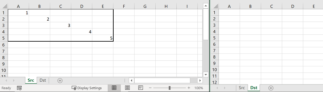
This is after using the VBA Range Copy function:
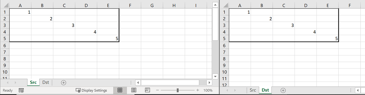
VBA Copy only on the UsedRanged
What to do however when you don’t want to bother with checking the used range of your source worksheet and just want to copy it whole? You can use the UsedRange attribute of the Source Worksheet – see example below.
Sub CopyUsedRange()
    Dim sourceWs As Worksheet, dstWs As Worksheet

    Set sourceWs = Sheets("Src")
    Set dstWs = Sheets("Dst")

    Call sourceWs.UsedRange.Copy(dstWs.Cells(1, 1))
End Sub
What’s the difference? In the above code snippet instead of copying a specific Range, we copy the entire UsedRange of the source Worksheet. The UsedRange is always any rectangle Range of cells that has been modified in any way in the Worksheet i.e. edited, color change, border etc. A UsedRange always has a starting and ending cell i.e. closest and furthest from A1 that have been modified. In my case the result was the same but the code above is much more convenient.
VBA Copy and paste values only
The VBA Copy Range function will copy the entire cell contents including formatting, borders, conditional formatting etc. Sometimes you want however to copy a variety of selected information or only the cell values without formatting. For this we would need to modify the macro above:
Sub CopyValuesOnly()
    Dim sourceWs As Worksheet, dstWs As Worksheet

    Set sourceWs = Sheets("Src")
    Set dstWs = Sheets("Dst")

    sourceWs.Range("A1:E5").Copy

    Call dstWs.Range("A1").PasteSpecial(Paste:=xlPasteValues)
End Sub
This time we modified the last two lines of the previous procedures. We first copy the selected Range from the source Worksheet. Then we use the VBA Range PasteSpecial function to paste the Range from the clipboard with only values to our destination Worksheet. This is the effect:
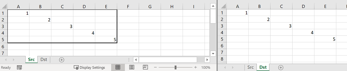
Conclusions
To VBA Copy Sheet data is simple and is regular use case. Do also check out my SQL AddIn for how to use SQL to copy data for one or multiple Worksheets.
Learning VBA unleashes the true potential of Microsoft Excel. This post shows you how to perform one of the more basic VBA tasks that Excel developers use frequently, that is copying a range of data from one worksheet to another worksheet.
Introduction
A common task to perform when developing Excel VBA scripts is copying data from one worksheet to another worksheet. This is used for all sorts of solutions, such as automating a report where you have imported data and want to get that data from the imported worksheet onto a reporting worksheet.
Example
The first step is to make a decision on the following:
- What is the range of data to copy, i.e. cells A1 to B20.
- What is the worksheet name containing the range of data to copy, i.e. “ImportSheet” or “Sheet2”.
- What is the worksheet name where the data will be copied.
- What is the starting location (cell) where the range will be copied, i.e. cell A1
An important part of this process is to make sure that the data you are copying is always in the same location, i.e. the same worksheet name and same range of cells.
For this example the answers to those four points above are:
- A1 to C13
- ImportSheet
- DataTable
- A1
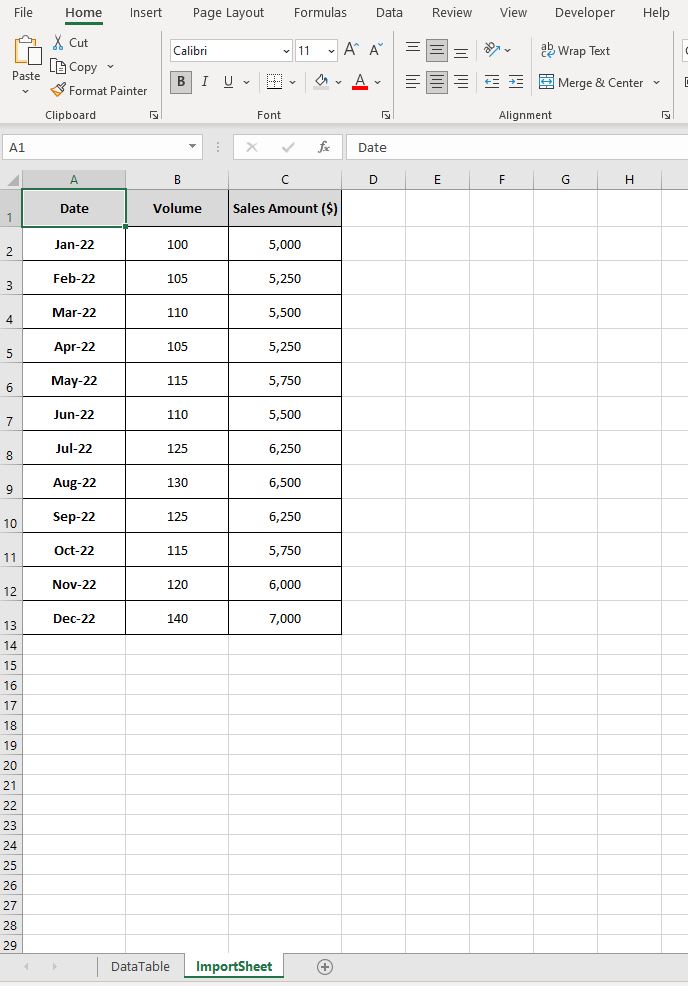
VBA time
The next step is to open the VBA window in Excel so the script can be written. To open the VBA window select the Developer tab from the Excel ribbon followed by clicking on the Visual Basic Icon on the far left, alternatively the shortcut command ALT + F11 will open the VBA window.
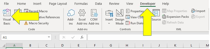
With the VBA window open the next step is to insert a new module, this is where the VBA script will be written. To do this click on Insert > Module on the top menu bar:
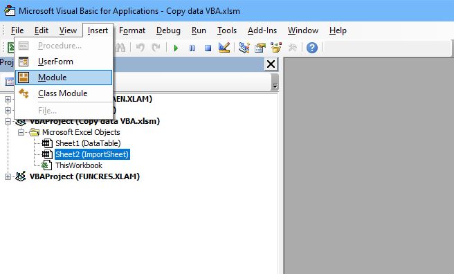
This will open a code window (module1) where the VBA script can be written:
The VBA code to copy the data from one worksheet to another can now be written.
VBA Code
The VBA code for to copy the data from the ImportSheet to the DataTable worksheet is as follows:
Sub CopyData()

Worksheets("ImportSheet").Range("A1:C13").Copy

Worksheets("DataTable").Range("A1").PasteSpecial

End Sub
Breaking down this VBA code line-by-line:
- Sub CopyData() – all VBA scripts need a name, Sub tells Excel this is a sub-procedure and CopyData is the name of this sub-procedure so can be changed to a different name. The brackets must be included at the end of this line of code.
- Worksheets(“ImportSheet”).Range(“A1:C13”).Copy – this line of code tells Excel what data to copy. For this example we want data on the worksheet called ImportSheet in the range A1 to C13 to be copied.
- Worksheets(“DataTable”).Range(“A1”).PasteSpecial – this line of code tells Excel where to copy the data. For this example the data is to be copied to the DataTable worksheet starting in cell A1.
- End Sub – this tells Excel the sub-procedure is finished and must be included.
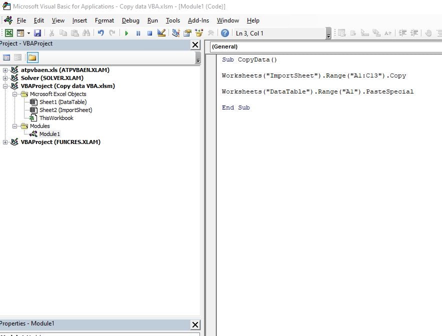
To run the VBA code click on the play button icon in the VBA window, alternatively pressing F5 will also run the code.
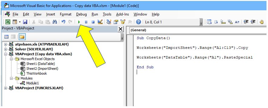
Now the data has been copied from the ImportSheet to the DataTable worksheet:
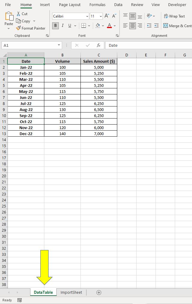
Keep Excelling,

Understanding VBA is the key to becoming an Excel power user and also a great way to have a career in Data Analysis, most companies use Excel in some way but few people understand VBA. There are more VBA posts on this site to help you along the way but for those wanting a reference book my favorite is VBA and Macros by Excel gurus Bill Jelen and Tracy Syrstad. You can check out a copy on Amazon by clicking the image below.
Copy paste in VBA is similar to what we do in the Excel worksheet:
- We can copy a value and paste it to another cell.
- We can use Paste Special to paste only the values. Similarly, in VBA, we use the copy method with range property to copy a value from one cell to another.
- We use the worksheet function Paste Special or the paste method to paste the value.
How to Copy Paste in VBA?
Below are some examples of how to copy-paste in Excel using VBA.
The basic thing we do in Excel is copy, cut, and paste the data from one cell to another. It requires no special introduction as well. However, learning VBA coding is important to understand the same concept in coding language. Copy paste in VBA is the routine task we do daily in Excel. To copy first, we need to decide which cell to copy.
Table of contents
- How to Copy Paste in VBA?
- Example #1 – Copy and Paste Values Using Range Object
- Example #2 – Copy to another Worksheet in the Same Workbook
- Example #3 – Copy from One Workbook to another Workbook
- Alternative Way for using Copy-Paste in VBA
- Top Ways of VBA Copy and Paste as Values
- Recommended Articles
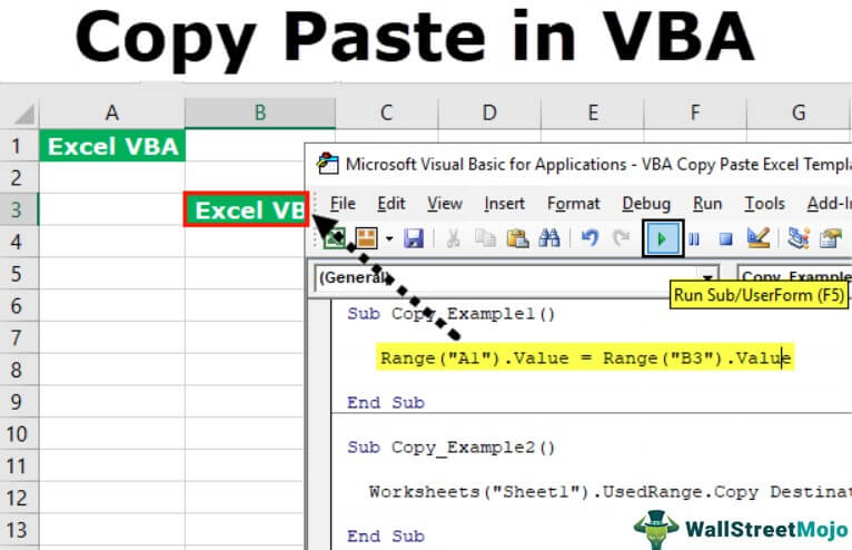
Example #1 – Copy and Paste Values Using Range Object
You can download this VBA Copy Paste Excel Template here – VBA Copy Paste Excel Template
Assume you have the word “Excel VBA” in cell A1.

For example, if you want to copy cell A1, we can use the VBA RANGE objectRange is a property in VBA that helps specify a particular cell, a range of cells, a row, a column, or a three-dimensional range. In the context of the Excel worksheet, the VBA range object includes a single cell or multiple cells spread across various rows and columns.read more.
Code:
Sub Copy_Example()

  Range ("A1").

End Sub

We can see all its properties and methods when you reference the cellCell reference in excel is referring the other cells to a cell to use its values or properties. For instance, if we have data in cell A2 and want to use that in cell A1, use =A2 in cell A1, and this will copy the A2 value in A1.read more. So, select the method “Copy.”
Code:
Sub Copy_Example()

  Range("A1").Copy

End Sub
After selecting the method, press the “Spacebar” key to see the argument of the copy method.

It shows “Destination.”
It is nothing, but where do you want to copy-paste values in VBA without selecting the PASTE method.
If we are pasting in the same sheet, we can select the cell using the Range object. For example, let us say if we want to paste the value in the B3 cell, we can put the destination as “Range(“B3″).”
Code:
Sub Copy_Example()

  Range("A1").Copy Destination:=Range("B3")

End Sub
It will copy the data from cell A1 and paste it into cell B3.
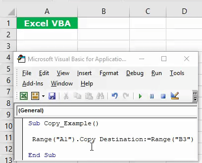
We can also use the below method to paste the data.
Code:
Sub Copy_Example()

  Range("A1").Copy
  Range("B3").Select
  ActiveSheet.Paste

End Sub
First, we will copy and select the data from cell A1 and paste it into cell B3.
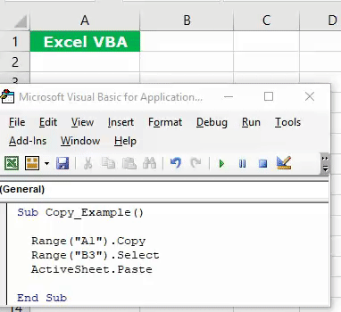
Example #2 – Copy to another Worksheet in the Same Workbook
Suppose we want to copy-paste the value from the different worksheets using VBA macro, then in the Destination argument. In that case, we need to reference the sheet name using the WORKSHEETS object and then mention the range of cells in that WORKSHEET. The below code will do the job.
Code:
Sub Copy_Example()

  Range("A1").Copy Destination:=Worksheets("Sheet2").Range("B3")

End Sub
If we want to copy the data from a specific sheet and paste it into another separate sheet, we need to mention both the names of the sheets.
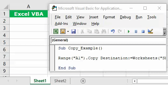
Firstly, we need to mention the copying sheet.
Worksheets("Sheet1").Range("A1").Copy
Then, in the “Destination argument,” we need to mention the targeted worksheet name and range of the cell.
Destination:=Worksheets("Sheet2").Range("B3")
So, the code should be like this.
Code:
Sub Copy_Example()

  Worksheets("Sheet1").Range("A1").Copy Destination:=Worksheets("Sheet2").Range("B3")

End Sub
Example #3 – Copy from One Workbook to another Workbook
We have seen how to copy from one worksheet to another worksheet in the same workbook. But, we can also do this from one workbook to another workbook.
Take a look at the below code.
Code:
SubCopy_Example()

  Workbooks("Book 1.xlsx").Worksheets("Sheet1").Range("A1").Copy
  Workbooks("Book 2.xlsx").Activate

  ActiveWorkbook.Worksheets("Sheet 2").Select
  ActiveSheet.Paste

End Sub
Firstly, it will copy the data from the worksheet “Sheet1” in the workbook “Book1.xlsx” from cell A1.
“Workbooks("Book 1.xlsx").Worksheets("Sheet1").Range("A1").Copy”
Then it will activate the workbook “Book 2.xlsx”.
Workbooks("Book 2.xlsx").Activate
The active workbook will select the worksheet “Sheet 2.”
ActiveWorkbook.Worksheets("Sheet 2").Select
Now in the active sheet, it will paste.
ActiveSheet.Paste
Alternative Way for using Copy-Paste in VBA
We have one more alternative way of having the data from one cell to another cell. Assume you have the word “Excel VBA” in cell A1 and you need the same to come in cell B3.

One method we have seen is using the VBA copy and paste method. Now, we will show you one of the alternative ways. Look at the below piece of code to understand.
Code:
Sub Copy_Example1()

  Range("A1").Value = Range("B3").Value

End Sub
The above says whatever the value is there in cell A1 should be equal to the value in cell B3.
Range("A1").Value = Range("B3").Value
Even though this is not a copy and paste method still adds more value to our coding knowledge.
Top Ways of VBA Copy and Paste as Values
Now, we will see different ways of VBA copy and paste values. Assume you are in cell A1 as shown in the below image.

- If we want to copy and paste, we need to reference the cell here. Rather, we can use the property of the Selection.Copy method.
Code:
Sub Copy_Example1()

  Selection.Copy Destination:=Range("B3")

End Sub
OR
Sub Copy_Example1()

  ActiveCell.Copy Destination:=Range("B3")

End Sub
- If you want to copy the entire used range of the worksheet, you can use the below code.
Code:
Sub Copy_Example2()

  Worksheets("Sheet1").UsedRange.Copy Destination:=Worksheets("Sheet2").Range("A1")

End Sub
It will copy the entire used range in the worksheet “Sheet1” and paste it into the worksheet “Sheet2.”
Recommended Articles
This article has been a guide to VBA Copy Paste. Here, we discuss the top ways to copy and paste in VBA, examples, and a downloadable Excel template. Below are some useful Excel articles related to VBA: –
- Copy Formatting in Excel
- Excel VBA Paste Values
- Excel VBA File Copy Function
- Excel VBA Paste