
Excel for Microsoft 365 Excel for Microsoft 365 for Mac Excel for the web Excel 2021 Excel 2021 for Mac Excel 2019 Excel 2019 for Mac Excel 2016 Excel 2016 for Mac Excel 2013 Excel 2010 Excel 2007 Excel for Mac 2011 More…Less
After you create an Excel table, you may only want the table style without the table functionality. To stop working with your data in a table without losing any table style formatting that you applied, you can convert the table to a regular range of data on the worksheet.

Important: In order to convert to a range, you must have an Excel table to start with. For more information, see Create or delete an Excel table.
-
Click anywhere in the table and then go to Table Tools > Design on the Ribbon.
-
In the Tools group, click Convert to Range.
-OR-
Right-click the table, then in the shortcut menu, click Table > Convert to Range.

Note: Table features are no longer available after you convert the table back to a range. For example, the row headers no longer include the sort and filter arrows, and structured references (references that use table names) that were used in formulas turn into regular cell references.
-
Click anywhere in the table and then click the Table tab.
-
Click Convert to Range.
-
Click Yes to confirm the action.
Note: Table features are no longer available after you convert the table back to a range. For example, the row headers no longer include the sort and filter arrows, and structured references (references that use table names) that were used in formulas turn into regular cell references.
Right-click the table, then in the shortcut menu, click Table > Convert to Range.
Note: Table features are no longer available after you convert the table back to a range. For example, the row headers no longer include the sort and filter arrows and the Table Design tab disappears.
Need more help?
You can always ask an expert in the Excel Tech Community or get support in the Answers community.
See Also
Video: Create and format tables
Need more help?
See all How-To Articles
This tutorial demonstrates how to convert a table to a data range (and the other way around) in Excel.
You have the option in Excel to create a table to work with data. Excel tables have features not available in a normal range, but the table format isn’t always best for what you’re doing.
Convert a Table to a Data Range
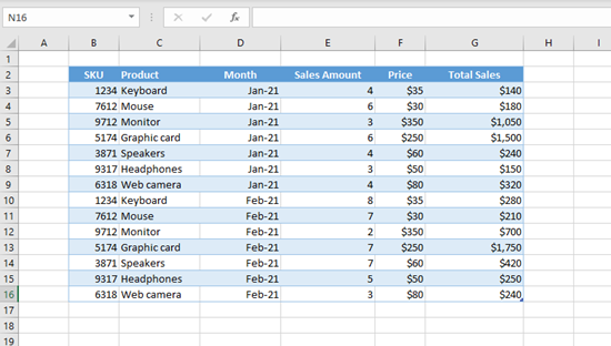
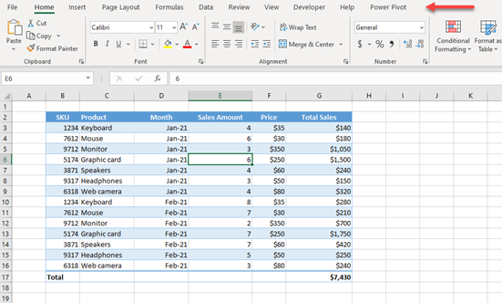
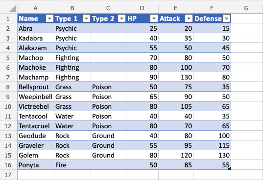
Say you have the following table with sales data and want to convert it to a normal range.
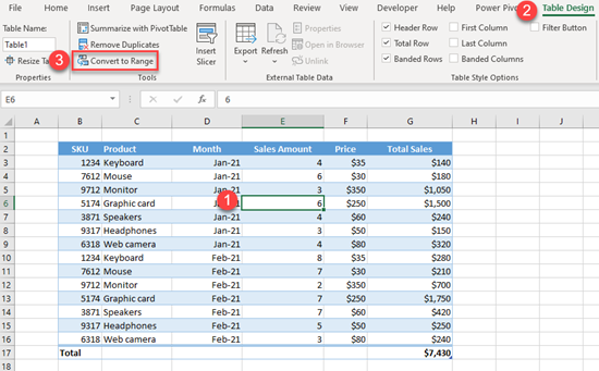
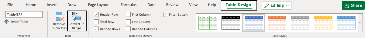
To convert this table to a data range, first click anywhere in the table. In the Ribbon, go to the Table Design tab, and click on Convert to Range.
As a result, you have the same data, but it’s no longer set up as an Excel table. To check this, click anywhere in the dataset, and see that now the Table Design tab doesn’t appear in the Ribbon.
Convert a Data Range to a Table
Now let’s see how to convert the data range back to a table.
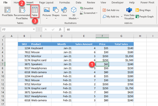
- First, click anywhere in the data range, then in the Ribbon, go to the Insert tab, and click on Table. The keyboard shortcut for this is CTRL + T.
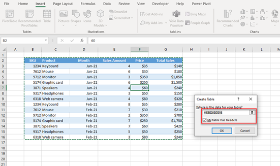
- In the pop-up screen, the whole data range is selected by default, and My table has headers is checked. Leave as is and click OK.
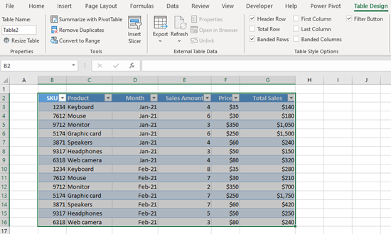
The data range is converted to a table, so when you select or click on the data, you get the Table Design tab on the Ribbon.
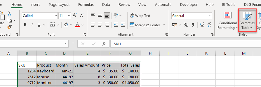
You can also use the Format as Table option to convert a normal data range into a table.
Convert an Excel table to a range of data
- Click anywhere in the table and then go to Table Tools > Design on the Ribbon.
- In the Tools group, click Convert to Range. -OR- Right-click the table, then in the shortcut menu, click Table > Convert to Range.
Contents
- 1 What is the shortcut for converting a range into a table in Excel?
- 2 How do you convert a table to a cell range?
- 3 Which is a valid reason you’d want to convert a table to a range?
- 4 How do you Deduplicate in Excel?
- 5 How do you convert data in Excel?
- 6 How do you flash fill in Excel?
- 7 How do I turn a table into a column in Excel?
- 8 What is an Xlookup in Excel?
- 9 What does #na mean in Excel?
- 10 What is range formula in Excel?
- 11 How do I set up index match in Excel?
- 12 How do I use conditional formatting in Excel?
- 13 How do you custom sort in Excel?
- 14 How do you convert a cell range to a table using a table style?
- 15 How do I convert a table to text in Excel?
- 16 How do I AutoFill in Excel using keyboard?
- 17 How do I format a range as a table with headers?
- 18 How do I enable Xlookup?
- 19 How do I enable Xlookup in Excel?
- 20 What is xmatch Excel?
What is the shortcut for converting a range into a table in Excel?
The keyboard shortcut for this is CTRL+T. In the pop-up screen, the whole data range is selected by default, and “My table has headers” is checked. We can leave this as-is and click OK. Our data range is converted to a table, so when we select or click on the data, we will get the Table Design tab in the Ribbon.
How do you convert a table to a cell range?
Convert an Excel table to a range of data
- Click anywhere in the table and then click the Table tab.
- Click Convert to Range.
- Click Yes to confirm the action. Note: Table features are no longer available after you convert the table back to a range.
Which is a valid reason you’d want to convert a table to a range?
Which is a valid reason you’d want to convert a table to a range? To prepare for importing new data from a non-Excel file. What is the difference between an Auto Outlined worksheet and a worksheet with multiple groups?
How do you Deduplicate in Excel?
Remove duplicate values
- Select the range of cells that has duplicate values you want to remove. Tip: Remove any outlines or subtotals from your data before trying to remove duplicates.
- Click Data > Remove Duplicates, and then Under Columns, check or uncheck the columns where you want to remove the duplicates.
- Click OK.
How do you convert data in Excel?
Convert a data type
- Select the Date column, select Home > Transform > Data Type, and then select the Date option. You can convert other numeric types, such as percentage or currency.
- To return the transformed data to the Excel worksheet, Select Home > Close & Load.
How do you flash fill in Excel?
You can go to Data > Flash Fill to run it manually, or press Ctrl+E. To turn Flash Fill on, go to Tools > Options > Advanced > Editing Options > check the Automatically Flash Fill box.
How do I turn a table into a column in Excel?
Select the table you want to transform into a single column. Click on Copy on the left-hand side of the “Professor Excel”-ribbon. Select the first cell from which Professor Excel should paste the columns underneath. Click on “Paste to Single Column” on the “Professor Excel” ribbon.
What is an Xlookup in Excel?
Use the XLOOKUP function to find things in a table or range by row.With XLOOKUP, you can look in one column for a search term, and return a result from the same row in another column, regardless of which side the return column is on.
What does #na mean in Excel?
no value is available
#N/A is the error value that means “no value is available.” Use NA to mark empty cells.
What is range formula in Excel?
A formula range is usually a reference to a range of cells, within which a formula persists consistently throughout the full range. A formula range, like a cell range, is defined by the reference of the upper left cell of the range and the reference of the lower right cell of the range.
How do I set up index match in Excel?
The INDEX MATCH formula is the combination of two functions in Excel.
Follow these steps:
- Type “=INDEX(” and select the area of the table, then add a comma.
- Type the row number for Kevin, which is “4,” and add a comma.
- Type the column number for Height, which is “2,” and close the bracket.
- The result is “5.8.”
How do I use conditional formatting in Excel?
Select the range of cells, the table, or the whole sheet that you want to apply conditional formatting to. On the Home tab, click Conditional Formatting. Click New Rule. Select a style, for example, 3-Color Scale, select the conditions that you want, and then click OK.
How do you custom sort in Excel?
To create a custom sort:
- Select a cell in the column you want to sort by.
- Select the Data tab, then click the Sort command.
- The Sort dialog box will appear.
- The Custom Lists dialog box will appear.
- Type the items in the desired custom order in the List entries: box.
- Click Add to save the new sort order.
How do you convert a cell range to a table using a table style?
Convert range to table in Excel
- Select the data range that you want to convert.
- Click Insert > Table, in the Create Table dialog box, check My table has headers if your data has headers, see screenshots:
- Then click OK, and your data range has been converted to the table format.
Convert a table to text
- Select the rows or table you want to convert to text.
- On the Layout tab, in the Data section, click Convert to Text.
- In the Convert to Text box, under Separate text with, click the separator character you want to use in place of the column boundaries.
- Click OK.
How do I AutoFill in Excel using keyboard?
Simply do the following:
- Select the cell with the formula and the adjacent cells you want to fill.
- Click Home > Fill, and choose either Down, Right, Up, or Left. Keyboard shortcut: You can also press Ctrl+D to fill the formula down in a column, or Ctrl+R to fill the formula to the right in a row.
Try it!
- Select a cell within your data.
- Select Home > Format as Table.
- Choose a style for your table.
- In the Create Table dialog box, set your cell range.
- Mark if your table has headers.
- Select OK.
How do I enable Xlookup?
INSTALLING THE XLOOKUP ADDIN [GKXLOOKUP]
- OPEN EXCEL.
- Go to OPTIONS>ADDINS.
- Select EXCEL ADD-INS.
- Click GO.
- A new dialog box will open as shown in the picture containing all the EXCEL ADD-INS list.
- We can select the Addins we want to activate.
- In our case we want to install the add in , so click BROWSE.
How do I enable Xlookup in Excel?
- Position the cell cursor in cell E4 of the worksheet.
- Click the Lookup & Reference option on the Formulas tab followed by XLOOKUP near the bottom of the drop-down menu to open its Function Arguments dialog box.
- Click cell D4 in the worksheet to enter its cell reference into the Lookup_value argument text box.
What is xmatch Excel?
The XMATCH function searches for a specified item in an array or range of cells, and then returns the item’s relative position. Here we’ll use XMATCH to find the position of an item in a list.
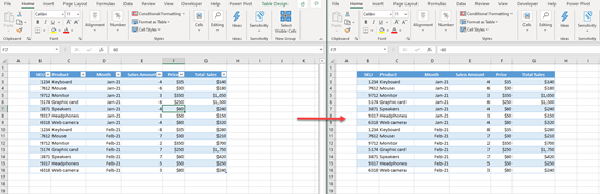
Excel allows us to convert a table to a range without losing the table style. A range means a regular set of data on the worksheet. This tutorial will walk all levels of Excel users through the easy steps of converting a table to a range while keeping all table style formatting.
 Figure 1 – Converted table to range
Data to Convert Table to Range
Before we can convert the table to a normal range, we must have created it. The table is created by clicking any cell within the range, clicking on the Insert tab, and clicking on Table.
 Figure 2 – Data to convert the table to a normal range
How to Convert a Table to a Range
We will do the following to convert table to a range.
- We will click any cell on the table
- We will go to the Design tab. We will click Convert to Range in the Tools group. On a Mac, we will do this on the Table tab.
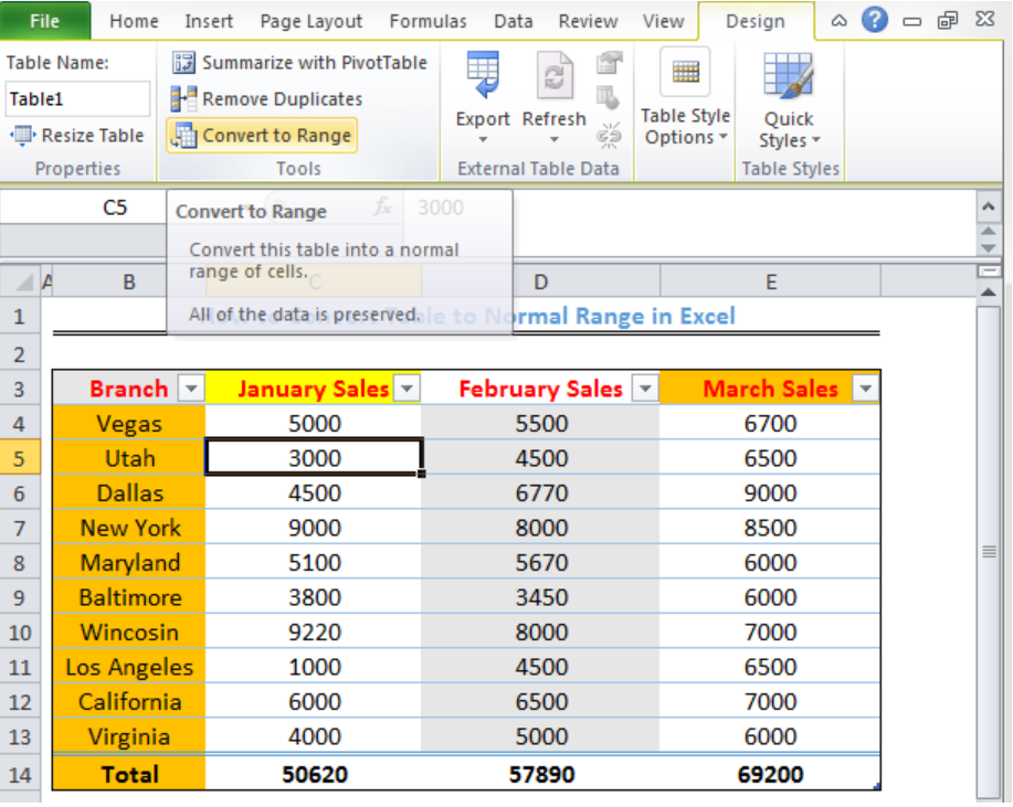 Figure 3 – Click Convert to Range
- We will receive a prompt. We will click Yes
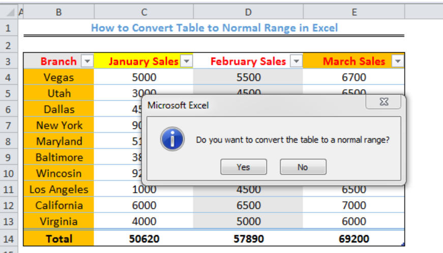 Figure 4 – Click Yes
- We will notice that the arrows on Row 3 will disappear
 Figure 5 – Converted table to range
Alternative Method to Convert a Table to a Range
- We will right-click on the table
- We will click Table
- We will click Convert to Range
Note
After we have converted to a normal range, the table functionalities such as the row headers and sort and filter arrows become unavailable.
Instant Connection to an Expert through our Excelchat Service
Most of the time, the problem you will need to solve will be more complex than a simple application of a formula or function. If you want to save hours of research and frustration, try our live Excelchat service! Our Excel Experts are available 24/7 to answer any Excel question you may have. We guarantee a connection within 30 seconds and a customized solution within 20 minutes.
Tables can be reversed and converted back to range.
Tables can be converted to ranges by selecting a cell in the table range and clicking on the Convert to Range command.
The command to convert to range is found in the Table Design tab, in the Tools group.
Example — Convert Table to Range
Type or copy the values to follow the example.
Convert the range into a table.
- Select a cell in the table range (
A1:F16)
- Click the Design Table tab ()
 )
)- Click the Convert to Range command ()
 )
)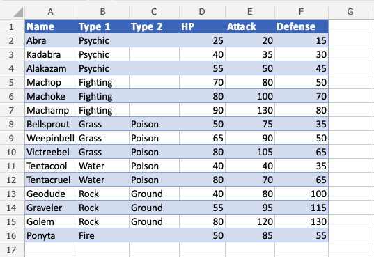
The table is now converted into a range and it no longer has the table options available.
Note: The cell formatting is kept for the range after the conversion.