
Excel for Microsoft 365 Excel for the web Excel 2021 Excel 2019 Excel 2016 Excel 2013 Excel 2010 Excel 2007 More…Less
Occasionally, dates may become formatted and stored in cells as text. For example, you may have entered a date in a cell that was formatted as text, or the data might have been imported or pasted from an external data source as text.
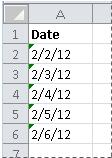
Dates that are formatted as text are left-aligned in a cell (instead of right-aligned). When Error Checking is enabled, text dates with two-digit years might also be marked with an error indicator:  .
.
Because Error Checking in Excel can identify text-formatted dates with two-digit years, you can use the automatic correction options to convert them to date-formatted dates. You can use the DATEVALUE function to convert most other types of text dates to dates.
If you import data into Excel from another source, or if you enter dates with two-digit years into cells that were previously formatted as text, you may see a small green triangle in the upper-left corner of the cell. This error indicator tells you that the date is stored as text, as shown in this example.
You can use the Error Indicator to convert dates from text to date format.
Notes: First, ensure that Error Checking is enabled in Excel. To do that:
-
Click File > Options > Formulas.
In Excel 2007, click the Microsoft Office button
 , then click Excel Options > Formulas.
 -
In Error Checking, check Enable background error checking. Any error that is found, will be marked with a triangle in the top-left corner of the cell.
-
Under Error checking rules, select Cells containing years represented as 2 digits.
 , then click Excel Options > Formulas.
Follow this procedure to convert the text-formatted date to a normal date:
-
On the worksheet, select any single cell or range of adjacent cells that has an error indicator in the upper-left corner. For more information, see Select cells, ranges, rows, or columns on a worksheet.
Tip: To cancel a selection of cells, click any cell on the worksheet.
-
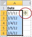
Click the error button that appears near the selected cell(s).
-
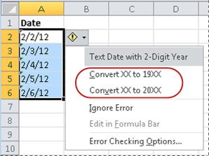
On the menu, click either Convert XX to 20XX or Convert XX to 19XX. If you want to dismiss the error indicator without converting the number, click Ignore Error.
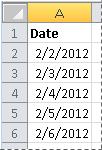
The text dates with two-digit years convert to standard dates with four-digit years.
Once you have converted the cells from text-formatted dates, you can change the way the dates appear in the cells by applying date formatting.
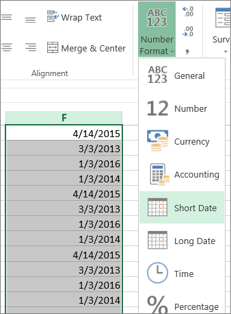
If your worksheet has dates that were perhaps imported or pasted that end up looking like a series of numbers like in the picture below, you probably would want to reformat them so they appear as either short or long dates. The date format will also be more useful if you want to filter, sort, or use it in date calculations.

-
Select the cell, cell range, or column that you want to reformat.
-
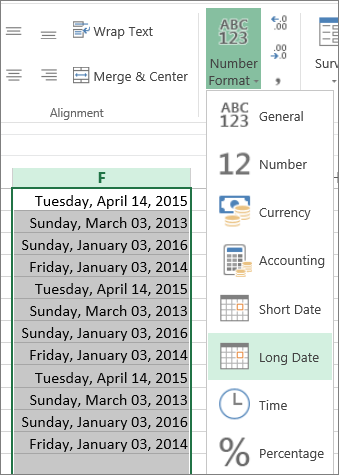
Click Number Format and pick the date format you want.
The Short Date format looks like this:
The Long Date includes more information like in this picture:
To convert a text date in a cell to a serial number, use the DATEVALUE function. Then copy the formula, select the cells that contain the text dates, and use Paste Special to apply a date format to them.
Follow these steps:
-
Select a blank cell and verify that its number format is General.
-
In the blank cell:
-
Enter =DATEVALUE(
-
Click the cell that contains the text-formatted date that you want to convert.
-
Enter )
-
Press ENTER, and the DATEVALUE function returns the serial number of the date that is represented by the text date.
What is an Excel serial number?
Excel stores dates as sequential serial numbers so that they can be used in calculations. By default, January 1, 1900, is serial number 1, and January 1, 2008, is serial number 39448 because it is 39,448 days after January 1, 1900.To copy the conversion formula into a range of contiguous cells, select the cell containing the formula that you entered, and then drag the fill handle
across a range of empty cells that matches in size the range of cells that contain text dates.
-
-
After you drag the fill handle, you should have a range of cells with serial numbers that corresponds to the range of cells that contain text dates.
-
Select the cell or range of cells that contains the serial numbers, and then on the Home tab, in the Clipboard group, click Copy.
Keyboard shortcut: You can also press CTRL+C.
-
Select the cell or range of cells that contains the text dates, and then on the Home tab, in the Clipboard group, click the arrow below Paste, and then click Paste Special.
-
In the Paste Special dialog box, under Paste, select Values, and then click OK.
-
On the Home tab, click the popup window launcher next to Number.
-
In the Category box, click Date, and then click the date format that you want in the Type list.
-
To delete the serial numbers after all of the dates are converted successfully, select the cells that contain them, and then press DELETE.
 across a range of empty cells that matches in size the range of cells that contain text dates.
Need more help?
You can always ask an expert in the Excel Tech Community or get support in the Answers community.
Need more help?
Want more options?
Explore subscription benefits, browse training courses, learn how to secure your device, and more.
Communities help you ask and answer questions, give feedback, and hear from experts with rich knowledge.
It is common to import data from other sources in Excel and it is also common to not get properly formatted data. For example, most of the time when we get data from other sources the date, time and numeric values are in text format. They need to be converted in the proper format. It is easy to convert numbers into excel numbers. But converting string into excel datetime may need a little bit of effort.
In this article, we will learn how you can convert text formatted date and time in excel date and time.
Generic Formula
Datetime_string: This is the reference of the string that contains the date and time.
The main functions in this generic formula are DATEVALUE and TIMEVALUE. Other functions are used to extract date string and time string if they are combined into one string. And yes, the cell that contains this formula should be formatted into datetime format otherwise you will see serial numbers that may confuse you.
Let’s see some examples to make things clear.
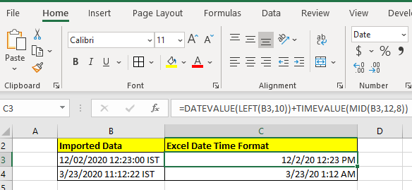
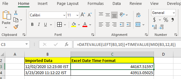
Example: Convert Imported Date and Time into Excel Datetime
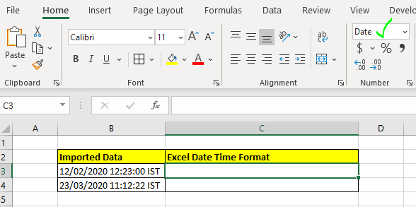
Here we have date and time combined into one string. We need to extract date and time separately and convert them into excel datetime.
Note that I have formatted C3 as a date so that the results I get are converted into dates and I don’t see a fractional number. (Secrets of excel date and time).
So let’s write the formula:
And it returns the date and time that excel considers as datetime, not string.
If you don’t change the cell formatting, this is what your result will look like.
This isn’t wrong. It is the serial number that represents that date and time. If you don’t know how the date and time are perceived by Excel, you can get complete clarity here.
How does it work?
This is simple. We use extraction techniques to extract date and time strings. Here we have LEFT(B3,10). This returns 10 characters from the left of the string in B3. Which is «12/02/2020». Now this string is supplied to the DATEVALUE function. And DATEVALUE converts the date string into its value. Hence we get 44167.
Similarly, we get time value using MID function (for extraction) and TIMEVALUE function.
The MID function returns 8 characters from the 12th position in string. Which is «12:23:00». This string is supplied to TIMEVALUE function that returns .51597.
Finally we add these numbers up. This gives us the number 44167.51597. When we convert the cell formatting to MM/DD/YYYY HH:MM AM/PM format we get the exact datetime.
In the above example, we had date and time concatenated together as a string. If you just have date as string without any extra text or string, you can use the DATEVALUE function alone to get the Date converted into excel date.
If you just have time as a string use the TIMEVALUE function
You can read about these functions by clicking on the function name in the formula.
So yeah guys, this is how you convert a date and time string into excel date time value. I hope this was helpful. If you have any doubts regarding this article or have any other query related Excel/VBA, ask me in the comment section below. I will be happy to help you.
Related Articles:
Convert Date and Time from GMT to CST : While working on Excel reports and Excel dashboards in Microsoft Excel, we need to convert Date and Time. In addition, we need to get the difference in timings in Microsoft Excel.
How to Convert Time to Decimal in Excel : We need to convert the time figures into decimals using a spreadsheet in Excel 2016. We can manipulate time in excel 2010, 2013 and 2016 using the function CONVERT, HOUR and MINUTE.
How to Convert date to text in Excel : In this article we learned how to convert text into date, but how do you convert an excel date into text. To convert an excel date into text we have a few techniques.
Converting Month Name to a Number in Microsoft Excel : When it comes to reports numbers are better than text. In Excel if you want to convert month names into numbers (1-12). Using the function DATEVALUE and MONTH you can easily convert months into numbers.
Excel convert decimal Seconds into time format : As we know, time in excel is treated as numbers. Hours, Minutes, and Seconds are treated as decimal numbers. So when we have seconds as numbers, how do we convert them into time format? This article got it covered.
Popular Articles:
50 Excel Shortcuts to Increase Your Productivity | Get faster at your task. These 50 shortcuts will make you work even faster on Excel.
How to use Excel VLOOKUP Function| This is one of the most used and popular functions of excel that is used to look up value from different ranges and sheets.
How to use the Excel COUNTIF Function| Count values with conditions using this amazing function. You don’t need to filter your data to count specific values. Countif function is essential to prepare your dashboard.
How to Use the SUMIF Function in Excel | This is another dashboard essential function. This helps you sum up values on specific conditions.
By default, all dates are stored as numbers in excel. If there is a time component, it gets stored as numeric with decimals. The following steps can be followed ( from ablebits.com) . There is a picture in the site to follow along with the steps.
How to change date format in Excel
In Microsoft Excel, dates can be displayed in a variety of ways. When it comes to changing date format of a given cell or range of cells, the easiest way is to open the Format Cells dialog and choose one of the predefined formats.
Select the dates whose format your want to change, or empty cells where you want to insert dates.
Press Ctrl+1 to open the Format Cells dialog. Alternatively, you can right click the selected cells and choose Format Cells… from the context menu.
In the Format Cells window, switch to the Number tab, and select Date in the Category list.
Under Type, pick a desired date format. Once you do this, the Sample box will display the format preview with the first date in your selected data.
Changing the date format in Excel
If you are happy for the preview, click the OK button to save the format change and close the window.
If the date format is not changing in your Excel sheet, most likely your dates are formatted as text and you have to convert them to the date format first.
Hope this helps.
Explanation
When date information from other systems is pasted or imported to Excel, it may not be recognized as a proper date or time. Instead, Excel may interpret this information as a text or string value only. In this example, the goal is to extract valid date and time information from a text string and convert that information into a datetime. It is important to understand that Excel dates and Excel times are numbers so at a high level, the main task is to convert a text value to the appropriate numeric value.
Date
To get the date, we extract the first 10 characters of the value with the LEFT function:
LEFT(B5,10) // returns "2015-03-01"
The result is text, so to get Excel to interpret as a date, we wrap LEFT in DATEVALUE, which converts the text into a proper Excel date.
Time
To get the time, we extract 8 characters from the middle of the text with the MID function:
MID(B5,12,8) // returns "12:28:45"
Again, the result is text. To get Excel to interpret this value as time, we wrap MID in TIMEVALUE, which converts the text into a proper Excel time.
Datetime
To get a final datetime, we just add the date value to the time value. The formula in E5 is:
=C5+D5
Once you have a valid datetime, use custom number formatting to display the value as desired.
All in one formula
Although this example extracts the date and time separately for clarity, you can combine formulas if you like. The following formula extracts the date and time, and adds them together in one step:
=LEFT(date,10)+MID(date,12,8)
Note that DATEVALUE and TIMEVALUE aren’t necessary in this case because the math operation (+) causes Excel to automatically coerce the text values to numbers.
Working with dates is a common task for many Excel users.
And sometimes, you can come across dates that are formatted as text (or look like dates but are not in the acceptable date formats, so Excel treat them as text strings).
Since dates are stored as numbers in the backend in Excel, it allows you to format dates in different ways as well as use them in calculations.
But when a date is stored as a text string in Excel, you won’t be able to use it in calculations or format it like a date.
In this tutorial, I will show you how to convert text into dates in Excel.
I will cover various scenarios where you may encounter a date that has either been formatted as text or is entered as a text string (and Excel doesn’t recognize that it’s a date).
Regular Date vs Text Date in Excel
Before I get into the methods on how to convert text to date in Excel, let me first explain what’s the difference between a date that is an acceptable format in Excel, and a date that is in the text format.
As I mentioned earlier, dates are stored as numbers in the back end in Excel, which makes it possible for us to use them in calculations just like numbers.
This also makes it possible for us to format dates and show it in different ways, which cannot be done when the date is entered as a text string or formatted as a text.
To give you an example, 01-Jan-2023 is an acceptable date format in Excel and if you enter this in a cell, it would be shown as a date, but it would be stored as 44927 in the backend (where 44927 is the number corresponding to the date 01-Jan-2023).
However, if you enter 01.Jan.2023, it would be entered as a text string because this is not an acceptable date format. This also means that you cannot use this in calculations because this has not been stored as a number in the back end
Below I have the table where I show the difference between an acceptable date format and a date in text format or entered as a text string.
| Date Stored as Number | Dates Stored as Text |
|---|---|
| Since these are numbers in the backend, these dates would be aligned to the left by default | Since these are text, these would be aligned to the right |
| These can be used in calculations | If dates are entered as a text string in Excel, you won’t be able to use this in formulas. However, if dates are formatted as text, then you can convert them back to numbers/dates, and then use them in formulas.
You can change the format to show these in other acceptable date formats (such as MM-DD-YYYY or DD-MM-YYYY or show only the month name or only the month and year)Since these are text, you cannot change the formatWhen you select cells containing the dates, you would be able to see Sum or Average in the status barSince these are text strings, you would only see the count value in the status bar |
Now let’s look at some of the methods you can use to convert text to dates in Excel
Convert Text to Date in Excel (with acceptable Date Formats)
First, we’ll look at scenarios where you have dates that are considered acceptable date format in Excel but are formatted as text in the cells.
For example, 01-Jan-2023 is an acceptable date format, and in case it has been formatted as text, you will be able to use the methods shown in this section to convert it back to date.
However, if a date is entered in a format that is not an accepted date format (such as 01.Jan.2023 or 8th Jan 2023), you will have to use methods covered later in this tutorial.
Using the DATEVALUE Function
Often, when you download your data from a database or you copy your data from a web page, you would notice that the dates have been formatted as text.
If your date is in the acceptable date format but has been formatted as text, you can easily convert it into the corresponding serial number by using the DATEVALUE function.
And once you have the number, you can easily format it as a date.
Below I have a data set where I have dates in column A that have been formatted as text and I want to convert these back to regular dates.

This can be done using the below DATEVAUE formula:
=DATEVALUE(A2)
Copy this formula to all the cells in column B.

When you use this formula, it gives you a numeric value, which corresponds to the date in cell A2.
So while we have got the text date converted into a number, we still need to format it so that it shows up as a date in the cell.
Below are the steps to format these numbers in column B to date:
- Select the cells that contain DATEVALUE results
- Click the Home tab

- In the Numbers group, click on the formatting drop-down
- Select the ‘Short date’ or ‘Long date’ format

The above steps would convert the text that you have in column A into serial numbers using the DATEVALUE function, and then these are formatted to show up as dates.

In case you need more control over how the dates are formatted, you can also use the Format Cells dialog box, which has a lot more date formatting options, as well as the option to create your own date format.
Also read: How to Change Date Format In Excel?
Using the VALUE Function
While the DATEVALUE function is built specifically to deal with dates that have been formatted as text, there is also a VALUE function that can deal with dates as well as non-dates.
VALUE takes any number that has been formatted as text and converts it back into numbers.
Below I have a data set where I have dates in column A that are in the text format, and I want to convert these back into regular dates.
Below is the VALUE formula that will do this for me:
=VALUE(A2)
Copy this formula to all the cells in column B.

And if you see the result as numeric values and not dates, you can format the cells to show these in dates using the below steps:
- Select the cells that contain VALUE formula results
- Click the Home tab
- In the Numbers group, click on the formatting drop-down
- Select the Short date or Long date format

Using Mathematical Operators (Add, Multiple, Double Minus, Division)
If you have a date in the format that Excel understands (even if it is in the text format), you will be able to use it in simple arithmetic calculations (such as addition or subtraction or multiplication or division).
We can use simple arithmetic calculations to convert the date that we have in the text format back into numeric format.
All you need to make sure is that you don’t end up changing the date in the calculation (which won’t happen if you add zero to the date or multiply the date by 1).
Below I have a data set where I have the dates in the text format in column A (but note that these are the dates that Excel would have considered as proper dates had they not been in the text format).
And here are some simple arithmetic calculations you can use in the adjacent column to get the numeric value of the date.
=A2+0
or
=A2*1
or
=A2/1
or
=--A2
You can use any of the above formulas and it would give you a numeric value in column B as shown below.

Note that we have the numeric value of the date in column A comma we can convert these back into date format.
Below are the steps to convert these numeric values into dates:
- Select the cells in column B that have the numeric value
- Click the Home tab
- In the number group, click on the drop-down
- Select the date format that you want to apply to the selected cells
In case you want to customize the date format further, select the cells in column B and then use the keyboard shortcut Control + 1 to open the Format Cells dialog box. Here you will get more date format options and you can also create your own custom date format if you want.
Using Paste Special
As explained in the previous method, you can convert a date that is formatted as text back into a numeric value by adding a zero to it.
While I’ve used a formula and got the result in a separate column in the above method, you can also do the same thing using the Paste Special dialog box.
Below I have a data set where I have the dates in the text format in column A and I want to convert these back to dates:
Below are the steps to convert dates in text format back into dates using the Paste Special technique:
- Copy any blank cell in the worksheet
- Select the dates in column A
- Right-click on the selection and then click on Paste Special option. This will open the Paste Special dialog box

- Select the ‘Values’ option in the ‘Paste’ category
- In the ‘Operation’ category, select the ‘Add’ option

- Click Ok
The above steps would instantly convert all the dates in column A into numeric values.

Now you can select these cells and change the format to show these numbers as dates.

How does this work?
When I copy a cell and then use paste special to add that cell to the dates in column A it’s essentially adding zero to these dates.
This addition does not change the numeric value of the date but it does convert the date value which is formatted as text into a numeric value that represents that date in the back end of Excel.
Also read: How to Multiply in Excel Using Paste Special
Convert Text to Date (with Format Not Recognized as Dates)
In all the examples covered above, I’ve shown you how to convert a date that is in the text format back into a date.
But so far, all our dates were in a format that Excel actually recognizes as a proper date.
It’s just that they have been formatted as text, so all we had to do was change the format back to date.
In this section, I’m going to show you some techniques that you can use when you have dates that are not recognized by Excel proper dates.
Such datasets often need more work, as we need to manipulate the data and convert it into proper date formats
By Changing the Delimiters in the Date
When there are dots or spaces instead of forward-slash or hyphens in a date, Excel would consider it as a text value as this is not an acceptable date format in Excel.
Below I have data set where I have the dates in column A where there are dots in between the day, month, and year number.

If you try to use the DATEVALUE or the VALUE function on this data, it will give you a value error (as Excel does not know how to convert this text string into a numeric value).

So the only way to convert this text value into data is by replacing the dot and changing the date into a proper date that Excel can recognize as a date.
Let me show you three different ways you can use to change the delimiters in the date in column A so that it can be used as a proper date in Excel.
Find and Replace
With Find and Replace, we can replace the dots in the date with a forward slash or hyphen/dash so that it will become a proper date format.
Below I have dates in column A that have dots as delimiters and I want to replace them with a forward slash or hyphen.
Here are the steps to do this:
- Select the cells in column A that have the date
- Click the Home tab
- In the Editing group, click on Find & Select
- Click on the ‘Replace’ option. This will open the Find and Replace dialog box

- In the ‘Find what’ field in the dialogue box, enter . (dot)
- In the ‘Replace with’ field, enter – dash

- Click on ‘Replace All’
The above steps would instantly change the dots in the dates into dashes, making the text values in column A into dates. Note that the dates also aligns to the right (while it was aligned to the left when it has dots instead of dashes).

Pro Tip: You can use the keyboard shortcut Control + H to open the ‘Find and Replace’ dialog box
Using Text to Columns
Another quick way to convert dates that are in text format into proper dates is by using the Text to Columns option.
Below I have a dataset where I have dates in column A that have dots as the delimiters and I want to convert these into regular dates that are recognizable by Excel.

Below are the steps to do this using Text to Columns:
- Select the cells in column A that have the dates
- Click the ‘Data’ tab

- In the ‘Data Tools’ group, click on the ‘Text to Columns’ option

- In Step 1 of the Convert Text to Columns Wizard, select Delimited and then click on Next

- In Step 2, make sure none of the delimiter option is selected, and then click on Next

- In Step 3, select the Date option and specify the destination cell (I would use $B$2 in this example). If you do not specify the destination cell, the data in the column would be overwritten

- Click on the Finish button
The above steps would instantly give you the dates in column B

It’s possible that the dates that you get in Column B are not in the format that you want.
So once you have the result, you can change the format by selecting the cells in Column B, holding the Control key, and pressing the 1 key. This will open the Format Cells dialog box where you can change the format of the dates.
SUBSTITUTE Function
You can also use the SUBSTITUTE function to replace the dots or dashes or any other delimiter with a forward slash or dash.
While the result of the SUBSTITUTE formula would be a text string, since it would be in an acceptable date format, we would be able to use DATEVALUE function to convert it into the numeric value of the corresponding date.
And once we have the numeric value, we can then format the cells to show the date in any format we want.
Below I have the data set where I have dates in column A that have dots as the delimiters, and I want to convert these into proper dates.
Build the formula that would give us the numeric value that represents the proper date:
=DATEVALUE(SUBSTITUTE(A2,".","-"))
Enter this formula in cell B2 and then copy it for all the other cells.

Once you have the results in column B, follow the below steps to convert these numbers back into dates:
- Select the cells in Column B that have the dates
- Click the Home tab
- In the Number group, click on the Format drop-down
- Select the ‘Short Date’ option
In case you want the dates to be shown in any other format, open the format cells dialog box and then choose from the multiple inbuild date formats or create your own custom date format.
Note that in the above formula, I had dots in the dates that I wanted to replace with dashes. In case you have any other delimiter (such as space), you need use that delimiter instead of the dot in the formula.
Convert Two Digit Year Text Date to Proper Date By Using Error Checking
Sometimes you may get a data set where the year is represented by two digits instead of the four digits in the date.
For example, instead of 01-Jan-2023, it would be 01-Jan-23
Thankfully, it only takes a click to get this sorted.
Below I have a data set in column A where I have the dates with two-digit year values and I want to convert these into proper date formats.

Here are the steps to do that:
- Select all the cells in column A that have the two-digit year date
- Click on the error-checking icon at the top right of the selection (it’s a yellow triangle icon)
- Click on ‘Convert XX to 20XX’ option

The above steps would change the dates and convert the two-digit year value to a four-digit year value.
Note that you can only use this if all the dates in your data set are of the same format (19XX or 20XX). In case there is a mix (for example in the case of date of birth), you will not be able to use this method
Using TEXT formulas
Sometimes you may get dates that have some additional text in the same cell.
For example, you can get a date where it includes the day name (such as Saturday, 08 Oct 2022) or a suffix after the day value (such as 8th October 2023 or 2nd October 2023).
In these cases, you first need to use some text formulas to clean the data and remove these unwanted text strings, and then try and convert these dates into their corresponding serial number (which can be done using the DATEVALUE function).
Let me show you a couple of common examples and how you can do this using simple text formulas:
When You Have Day Name in the Date
Below I have a data set where I have the day name before the date in column A, and I want to convert these dates in column A into proper date format.

Here is the formula that will do this for me:
=DATEVALUE(RIGHT(A2,LEN(A2)-FIND(" ",A2)))
Enter this formula in cell B2 and then copy it for all the cells in column B.

In the above data set, the day name is always followed by a comma and a space character.
Since this is the same in all the cells in the data set, I have used the above formula to first identify the position of the first space character (using the FIND function).
Once I know the position of the first space character, I used the RIGHT function to extract everything which is to the right of that space character.
And since the result of the RIGHT function is still a text string, I’ve used the DATEVALUE function to get the serial number of the date.
Once you have the serial number of the date, you can format the cell to show it in the short or long date format (your option is available in the Home tab in the formatting drop-down)
When You have Suffix After the Day Value in the Date
Below are the data set where I have a suffix (such as ‘th’, ‘rd’, ‘nd’, ‘st’) after the day value.

Because of this, the date is considered as a text string in Excel, and to convert this date in the text format back into the date format, I will have to remove the suffix from these cells.
Below is the formula that will do this for me:
DATEVALUE(SUBSTITUTE(SUBSTITUTE(SUBSTITUTE(SUBSTITUTE(A2,"th",""),"st",""),"rd",""),"nd",""))
Enter this formula in cell B2 and then copy it for all the cells in column B.

In the above formula, I have used the SUBSTITUTE function to remove each of these suffix values and replace these with blanks.
Since there are four such values (th, st, rd, nd), I had to use the SUBSTITUTE function four times.
The result of one SUBSTITUTE function is fed into another SUBSTITUTE function so that in the end we get the result where any of these four suffixes would be removed.
Once the suffixes are removed, we have used the DATEVALUE function to get the serial number of the date so that we can convert it back into the proper date format
Convert 8 Digit Date in MMDDYYYY format to Date
Below I have a data set where I have the dates in the DDMMYYYY format, where there is no space or delimiter between any of the digits.

Since the above dataset follows a consistent pattern (where the first two digits are always the day value, the next two digits are the month value, and the last four digits are the year value), we can use simple text formulas to extract these digits and specify them as the day, month and year values.
Here is the formula that will do this for me:
=DATE(RIGHT(A2,4),MID(A2,3,2),LEFT(A2,2))
Enter this formula in cell B2 and then copy it for all the cells in column B.

The above formula uses the RIGHT, MID, and LEFT functions to extract the year, month, and day values respectively,
And then these are used within the DATE function to construct a proper date in Excel.
In this tutorial, I showed you how to convert text to date in Excel using various techniques.
The method you use would depend on whether your date is in a format that Excel would recognize as a proper date or not.
If it is in a proper date format and is being considered as a text string in Excel, you can use formulas such as DATEVALUE or VALUE to get the serial number of the date and then format it to show as a short or long date.
You can also use simple arithmetic operators or Paste Special operation techniques to quickly convert dates that are formatted as text into serial numbers corresponding to that date.
And in case your dates are in a format that is not recognized by Excel a date, you will need to do some text manipulation using simple text formulas or functionalities such as Find and Replace or Text to Columns.
I hope you found this Excel tutorial useful.
Other Excel tutorials you may also like:
- How to Compare Dates in Excel (Greater/Less Than, Mismatches)
- Combine Date and Time in Excel (Easy Formula)
- Convert Date to Text in Excel – Explained with Examples
- How to Convert Serial Numbers to Dates in Excel
- Convert Text to Numbers in Excel
- How to Convert Numbers to Text in Excel