
Convert Data Into a Table in Excel
This page will show you how to convert Excel data into a table.
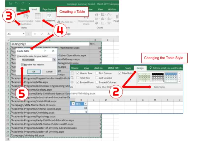
Creating a Table within Excel
- Open the Excel spreadsheet.
- Use your mouse to select the cells that contain the information for the table.
- Click the «Insert» tab > Locate the «Tables» group.
- Click «Table». A «Create Table» dialog box will open.
- If you have column headings, check the box «My table has headers».
- Verify that the range is correct > Click [OK].
- Resize your columns to make the headings visible.
Changing the Table Style
- Click on a cell in the table to activate the «Table Tools» tab.
- Click the «Design» tab > Locate the «Table Styles» group.
- Choose a style/color option that appeals to you. (Hover over the various table styles to see a live preview.)
Keywords: Office, color, colors, filter, sort, rows, columns, apply, enhance, table
Share This Post
-
Facebook
-
Twitter
-
LinkedIn
Blog Resources
Cedarville offers more than 150 academic programs to grad, undergrad, and online students. Cedarville is known for its biblical worldview, academic excellence, intentional discipleship, and authentic Christian community.

Loading…
The Excel Table is a relatively seldom used and underrated feature in Excel. But in today’s article, we’ll show you the advantages of its use. It makes it easy for a user to manage data if it is in a tabular format.
Converting a data range into a table makes its usage even easier. After this little intro, let’s see the step-by-step tutorial!
Suppose our data is in tabular format. In the next few steps, we’ll show you how to convert them into an Excel Table.
1. Select the worksheet range that contains the data set.
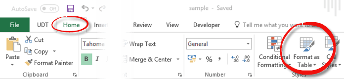
2. After this, choose the Home tab, then go to the Format as Table icon.
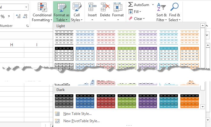
3. As you can see in the picture, many pre-set arrangements and color themes are available. Choose the one you like!
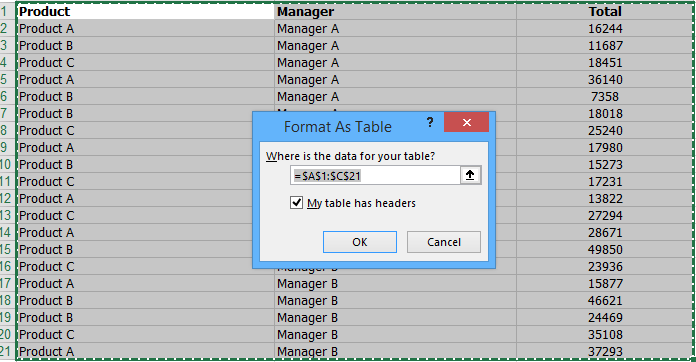
4. The Format as Table dialogue box contains the following information. First, “Where is the data for your table?”
The answer is obvious; we can see the range we want to convert into Table format. We always check this before we start the conversion to ensure the right range!
If our data table has headers, we need to check the box “My Table has headers.” Excel will automatically insert headers into the first row if your data doesn’t have headers.
5. Click OK.
Shortcut tips: use the Ctrl+T keyboard shortcut; this makes the conversion a lot faster. If you highlight the data table as an effect of the shortcut, you will immediately see the “Format as Table” dialogue box; no need to look for it on the ribbon.
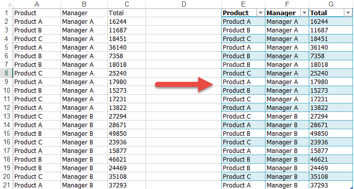
When your tabular data is converted into Excel Table, your data will look as shown below.
The most important changes are: the header got a darker shade, and the color of the rows is different. Data filters are enabled on the header. Note that the data hasn’t changed, only the design.
How to convert data from the table into a tabular format back?
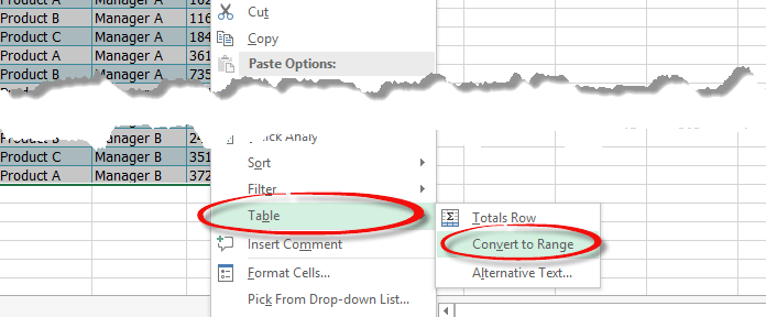
Sometimes we would like to convert the Excel Table to its original tabular range format. Let’s see what we have to do! Highlight the range, or easier to click anywhere on the table. Right-click, and from the Table menu, click on the “Convert to Range” icon.
Note that when you convert the Excel Table to a range, it no longer has the properties of an Excel Table (discussed below), however, it retains the formatting.
Useful Table Features in Excel
So we have seen how to create a table. Now let’s see the useful functions it enables.
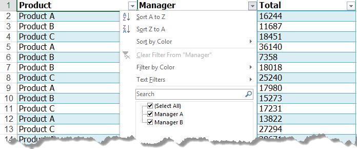
• The created table automatically makes a header that enables the sort and filter options.
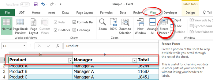
• If our list or range is long and stretches beyond the visible screen, the header remains at the top when scrolling. It works similarly to the “Freeze Top Row” function.
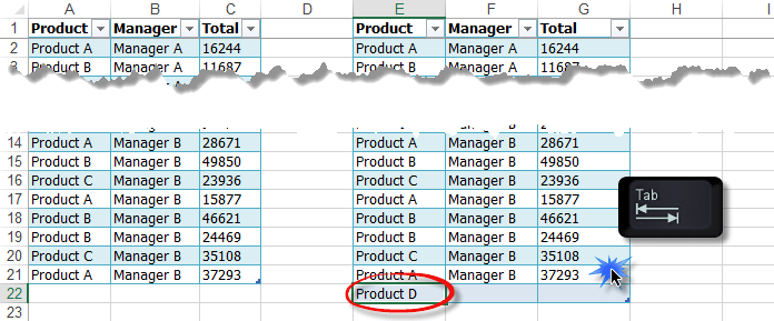
• And now let’s see one of our favorite functions! When we reach the bottom of our range but want to add additional rows, simply use the TAB button. This adds new rows to the table.
• Now, let’s examine the case when we need to do calculations with the table. When new rows added, Excel automatically figures them into the calculation.
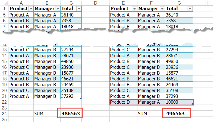
Table Design – Overview
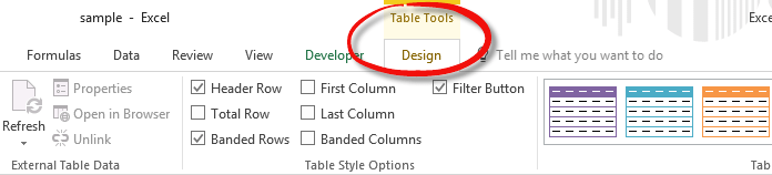
If you are involved with Excel, you know it is easy to customize. We can dress it any way we want to. Click on any cell in the Table, and an additional button, “Table Tools Design” will appear on the ribbon. This is optional and can be seen only when working with tables.
When you click on the Design tab, several options are available.
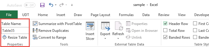
• Properties: Properties is one of the most useful tools of the group, we can give a unique name to our table. This is in the Table name box. We can use it as a reference. Re-size it and the name – of course – will remain the same.
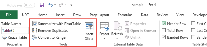
Tools: The following options are available:
- Summarize with Pivot Table: This simply creates a pivot table using the Excel table’s data.
- Remove Duplicates: In our article about data cleansing, we detailed how to quickly remove duplicates.
- Convert to Range: With the use of this option, we can convert an Excel Table into a regular range.
- Insert Slicer (only in Excel 2013 and 2016): Slicer can be familiar with our Pivot tables subject. Its function is similar here. Very useful in filtering and arranging data using a single click. A splendid addition to a dashboard.
External Table Data
This menu exports and refreshes data.
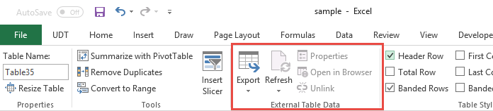
Table Style Options
These are design elements. There are more variants to customize the created table.
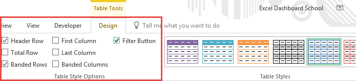
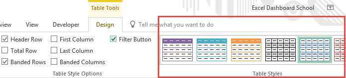
Table Styles
When we don’t have the time to create personal styles, here we have many pre-defined themes at our disposal. The variety is wide, everyone can find the perfect one. But also we can make our style by selecting the “New Table Style” option. It is the fastest method if you want to highlight every other row.
Conclusion
In a summary, we can say that with the use of Excel Table we can have our data in the appropriate structure. Further work is very simple with it. Its biggest advantage is that we can easily expand the original list/range without additional calculations. We recommend its use.
The following step-by-step example shows how to convert an Excel pivot table to a data table.
Step 1: Enter the Data
First, let’s enter the following sales data for three different stores:

Step 2: Create the Pivot Table
To create a pivot table, click the Insert tab along the top ribbon and then click the PivotTable icon:

In the new window that appears, choose A1:C16 as the range and choose to place the pivot table in cell E1 of the existing worksheet:

Once you click OK, a new PivotTable Fields panel will appear on the right side of the screen.
Drag the Store field to the Rows box, then drag the Product field to the Columns box, then drag the Quantity field to the Values box:

The pivot table will automatically be populated with the following values:

Step 3: Convert Pivot Table to Table
To convert this pivot table to an ordinary data table, simply select the entire pivot table (in this case, we select the range E1:I6) and press Ctrl+C to copy the data.

Then right click the cell where you’d like to paste the data (we’ll choose cell E8) and click the option titled Paste Values:

The values from the pivot table will automatically be pasted as regular data values, starting in cell E8:

Notice that this table doesn’t contain any of the fancy formatting or dropdown filters that were in the pivot table.
We’re simply left with a table of regular data values.
Additional Resources
The following tutorials explain how to perform other common tasks in Excel:
How to Create Tables in Excel
How to Group Values in Pivot Table by Range in Excel
How to Group by Month and Year in Pivot Table in Excel
Excel for Microsoft 365 Excel for Microsoft 365 for Mac Excel for the web Excel 2021 Excel 2021 for Mac Excel 2019 Excel 2019 for Mac Excel 2016 Excel 2016 for Mac Excel 2013 Excel 2010 Excel 2007 Excel for Mac 2011 More…Less
After you create an Excel table, you may only want the table style without the table functionality. To stop working with your data in a table without losing any table style formatting that you applied, you can convert the table to a regular range of data on the worksheet.

Important: In order to convert to a range, you must have an Excel table to start with. For more information, see Create or delete an Excel table.
-
Click anywhere in the table and then go to Table Tools > Design on the Ribbon.
-
In the Tools group, click Convert to Range.
-OR-
Right-click the table, then in the shortcut menu, click Table > Convert to Range.

Note: Table features are no longer available after you convert the table back to a range. For example, the row headers no longer include the sort and filter arrows, and structured references (references that use table names) that were used in formulas turn into regular cell references.
-
Click anywhere in the table and then click the Table tab.
-
Click Convert to Range.
-
Click Yes to confirm the action.
Note: Table features are no longer available after you convert the table back to a range. For example, the row headers no longer include the sort and filter arrows, and structured references (references that use table names) that were used in formulas turn into regular cell references.
Right-click the table, then in the shortcut menu, click Table > Convert to Range.
Note: Table features are no longer available after you convert the table back to a range. For example, the row headers no longer include the sort and filter arrows and the Table Design tab disappears.
Need more help?
You can always ask an expert in the Excel Tech Community or get support in the Answers community.
See Also
Video: Create and format tables
Need more help?
Skip to content
![]()
Excel has a data table format, called “Data Tables” (or “Excel Tables”) were introduced in Excel 2007. They were supposed to simplify the work with data in Excel. I like to use them quite a lot because they often make the work with functions (especially complex SUMIFS functions), quite simple. In this article I describe, how to convert an Excel table to normal cell range.
In a hurry? Click once on a cell in your data table, go to the table tools ribbon and click on “Convert to Range“.
What is an Excel table in?
First of all: We are not talking about the data table that are part of the What-If Analysis functions on the data ribbon. For the analyse function also called data table please refer to this article.
A table (which is also called “Excel table”) offers a structured way to organize your data. It has some advantages and disadvantages towards normal cell ranges:
- A table (or “Excel Table”) offers some built-in filtering, sorting, row shading and so on.
- It (by default) uses the same formula for the complete row. So, it’s not possible to use a different formula in a single cell within the data table.
Steps for converting an Excel Table into a normal table
Method 1: Convert table to range via the ribbon
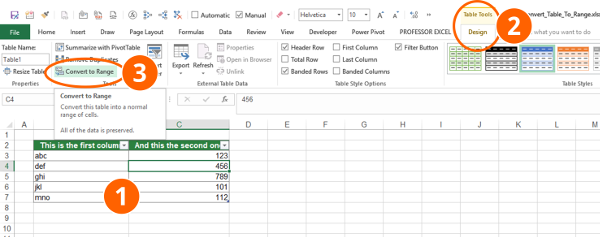
There are two necessary steps for changing your table to a normal range (the numbers are corresponding to the picture):
- Click on a cell within the Data Table.
- The yellow Table Tools (“Design”) ribbon is now visible. Click on it.
- A little bit hidden: “Convert to Range” is located under the “Tools” group. Click on it and confirm with YES.
Please note that the formatting (for example the row background pattern) might be lost.
Method 2: Right-click on the table to convert it to range
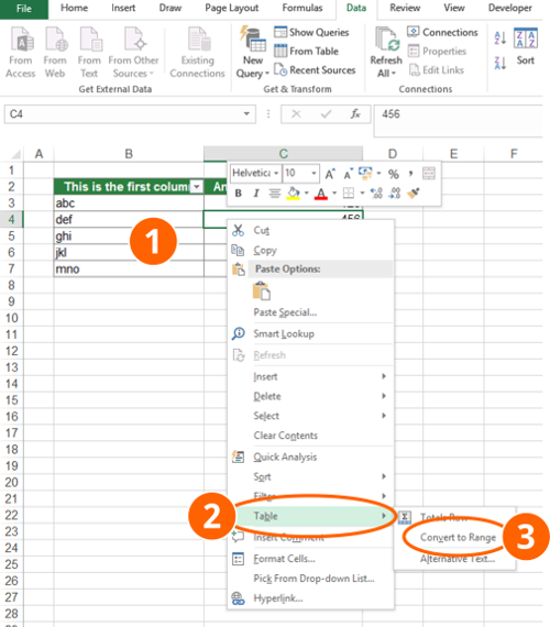
The second method is even faster.
- Right-click on a cell within the Data Table.
- Scroll down to “Table” and click on “Convert to Range”. Confirm with YES.
Do you want to boost your productivity in Excel?
Get the Professor Excel ribbon!

Add more than 120 great features to Excel!
Insert an Excel table
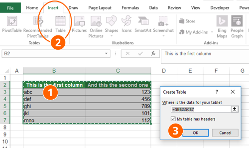
Is also not difficult to convert a normal table into a data table (or Excel table).
- Select the cells you want to convert. Usually it’s also fine to just select one cell and Excel detects the complete table range. But the safer way is to select the entire cell range.
- Go to the “Insert” ribbon and click on “Table”.
- Check if the selected cell range is correct and click on OK.
There is also a keyboard shortcut for inserting Excel tables: Press Ctrl + T on the keyboard.
Image by Pexels from Pixabay

Henrik Schiffner is a freelance business consultant and software developer. He lives and works in Hamburg, Germany. Besides being an Excel enthusiast he loves photography and sports.
We use cookies on our website to give you the most relevant experience by remembering your preferences and repeat visits. By clicking “Accept”, you consent to the use of ALL the cookies.
.