
Excel for Microsoft 365 Excel for the web Excel 2021 Excel 2019 Excel 2016 Excel 2013 Excel 2010 Excel 2007 More…Less
Occasionally, dates may become formatted and stored in cells as text. For example, you may have entered a date in a cell that was formatted as text, or the data might have been imported or pasted from an external data source as text.
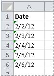
Dates that are formatted as text are left-aligned in a cell (instead of right-aligned). When Error Checking is enabled, text dates with two-digit years might also be marked with an error indicator:  .
.
Because Error Checking in Excel can identify text-formatted dates with two-digit years, you can use the automatic correction options to convert them to date-formatted dates. You can use the DATEVALUE function to convert most other types of text dates to dates.
If you import data into Excel from another source, or if you enter dates with two-digit years into cells that were previously formatted as text, you may see a small green triangle in the upper-left corner of the cell. This error indicator tells you that the date is stored as text, as shown in this example.
You can use the Error Indicator to convert dates from text to date format.
Notes: First, ensure that Error Checking is enabled in Excel. To do that:
-
Click File > Options > Formulas.
In Excel 2007, click the Microsoft Office button
 , then click Excel Options > Formulas.
 -
In Error Checking, check Enable background error checking. Any error that is found, will be marked with a triangle in the top-left corner of the cell.
-
Under Error checking rules, select Cells containing years represented as 2 digits.
 , then click Excel Options > Formulas.
Follow this procedure to convert the text-formatted date to a normal date:
-
On the worksheet, select any single cell or range of adjacent cells that has an error indicator in the upper-left corner. For more information, see Select cells, ranges, rows, or columns on a worksheet.
Tip: To cancel a selection of cells, click any cell on the worksheet.
-
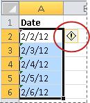
Click the error button that appears near the selected cell(s).
-
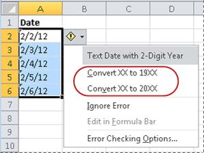
On the menu, click either Convert XX to 20XX or Convert XX to 19XX. If you want to dismiss the error indicator without converting the number, click Ignore Error.
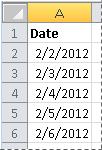
The text dates with two-digit years convert to standard dates with four-digit years.
Once you have converted the cells from text-formatted dates, you can change the way the dates appear in the cells by applying date formatting.
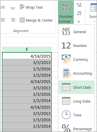
If your worksheet has dates that were perhaps imported or pasted that end up looking like a series of numbers like in the picture below, you probably would want to reformat them so they appear as either short or long dates. The date format will also be more useful if you want to filter, sort, or use it in date calculations.

-
Select the cell, cell range, or column that you want to reformat.
-
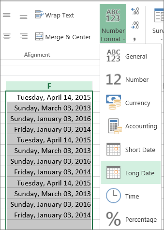
Click Number Format and pick the date format you want.
The Short Date format looks like this:
The Long Date includes more information like in this picture:
To convert a text date in a cell to a serial number, use the DATEVALUE function. Then copy the formula, select the cells that contain the text dates, and use Paste Special to apply a date format to them.
Follow these steps:
-
Select a blank cell and verify that its number format is General.
-
In the blank cell:
-
Enter =DATEVALUE(
-
Click the cell that contains the text-formatted date that you want to convert.
-
Enter )
-
Press ENTER, and the DATEVALUE function returns the serial number of the date that is represented by the text date.
What is an Excel serial number?
Excel stores dates as sequential serial numbers so that they can be used in calculations. By default, January 1, 1900, is serial number 1, and January 1, 2008, is serial number 39448 because it is 39,448 days after January 1, 1900.To copy the conversion formula into a range of contiguous cells, select the cell containing the formula that you entered, and then drag the fill handle
across a range of empty cells that matches in size the range of cells that contain text dates.
-
-
After you drag the fill handle, you should have a range of cells with serial numbers that corresponds to the range of cells that contain text dates.
-
Select the cell or range of cells that contains the serial numbers, and then on the Home tab, in the Clipboard group, click Copy.
Keyboard shortcut: You can also press CTRL+C.
-
Select the cell or range of cells that contains the text dates, and then on the Home tab, in the Clipboard group, click the arrow below Paste, and then click Paste Special.
-
In the Paste Special dialog box, under Paste, select Values, and then click OK.
-
On the Home tab, click the popup window launcher next to Number.
-
In the Category box, click Date, and then click the date format that you want in the Type list.
-
To delete the serial numbers after all of the dates are converted successfully, select the cells that contain them, and then press DELETE.
 across a range of empty cells that matches in size the range of cells that contain text dates.
Need more help?
You can always ask an expert in the Excel Tech Community or get support in the Answers community.
Need more help?
Want more options?
Explore subscription benefits, browse training courses, learn how to secure your device, and more.
Communities help you ask and answer questions, give feedback, and hear from experts with rich knowledge.
Watch video – Convert Date to Text in Excel
Date and Time in Excel are stored as numbers. This enables a user to use these dates and time in calculations. For example, you can add a specific number of days or hours to a given date.
However, sometimes you may want these dates to behave like text. In such cases, you need to know how to convert the date to text.
Below is an example where dates are combined with text. You can see that the dates don’t retain their format and show up as numbers in the combined text.

In such situations, it’s required to convert a date into text.
Convert Date to Text in Excel
In this tutorial, you’ll learn three ways to convert the date to text in Excel:
- Using the Text Function
- Using the Text to Column feature
- Using the Copy-Paste method
Convert Date to Text using Text Function
TEXT function is best used when you want to display a value in a specific format. In this case, it would be to display the date (which is a number) in the date format.
Let’s first see how the text function works.
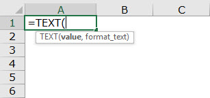
Here is the syntax:
=TEXT(value, format_text)
It takes two arguments:
- value – the number that you want to convert into text. This can be a number, a cell reference that contains a number, or a formula result that returns a number.
- format_text – the format in which you want to display the number. The format needs to be specified within double quotes.
Using the Text function requires a basic understanding of the formats that you can use in it.
In the case of dates, there are four parts to the format:
- day format
- month format
- year format
- separator
Here are the formats you can use for each part:
- Day Format:
- d – it shows the day number without a leading zero. So 2 will be shown as 2 and 12 will be shown as 12.
- dd – it shows the day number with a leading zero. So 2 will be shown as 02, and 12 will be shown as 12
- ddd – it shows the day name as a three letter abbreviation of the day. For example, if the day is a Monday, it will show Mon.
- dddd – it shows the full name of the day. For example, if it’s Monday, it will be shown as Monday.
- Month Format:
- m – it shows the month number without a leading zero. So 2 will be shown as 2 and 12 will be shown as 12.
- mm – it shows the month number with a leading zero. So 2 will be shown as 02, and 12 will be shown as 12
- mmm – it shows the month name as a three letter abbreviation of the day. For example, if the month is August, it will show Aug.
- mmmm – it shows the full name of the month. For example, if the month is August, it will show August.
- Year Format:
- yy – it shows the two digit year number. For example, if it is 2016, it will show 16.
- yyyy – it shows the four digit year number. For example, if it is 2016, it will show 2016.
- Separator:
- / (forward slash): A forward slash can be used to separate the day, month, and year part of a date. For example, if you specify “dd/mmm/yyyy” as the format, it would return a date with the following format: 31/12/2016.
- – (dash): A dash can be used to separate the day, month, and year part of a date. For example, if you specify “dd-mmm-yyyy” as the format, it would return a date with the following format: 31-12-2016.
- Space and comma: You can also combine space and comma to create a format such as “dd mmm, yyyy”. This would show the date in the following format: 31 Mar, 2016.
Let’s see a few examples of how to use the TEXT function to convert date to text in Excel.
Example 1: Converting a Specified Date to Text
Let’s again take the example of the date of joining:
Here’s the formula that will give you the right result:
=A2&"'s joining date is "&TEXT(B2,"dd-mm-yyyy")

Note that instead of using the cell reference that has the date, we have used the TEXT function to convert it into text using the specified format.
Below are some variations of different formats that you can use:
You can experiment with other formats as well and create your own combinations.
Also read: How to Convert Text to Date in Excel (8 Easy Ways)
Example 2: Converting Current Date to Text
To convert the current date into text, you can use the TODAY function along with the TEXT function.
Here is a formula that will do it:
="Today is "&TEXT(TODAY(),"dd/mm/yyyy")
This could be useful in dashboards/reports, where as soon as the file is opened (or any changes are made), the date refreshes to show the current date.

Convert Date to Text using Text to Column
If you’re not a fan of Excel formulas, there is another cool way to quickly convert date to text in Excel – the Text to Column feature.
Suppose you have a dataset as shown below and you want to convert these dates into text format:

Here are the steps to do this:
- Select all the cells that contain dates that you want to convert to text.
- Go to Data –> Data Tools –> Text to Column.

- In the Text to Column Wizard, make the following selections:

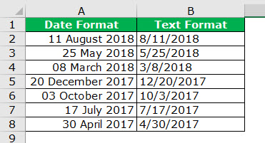
This would instantly convert the dates into text format.

Note: There is a difference in the format of the dates in the two columns. While the original format had dd mmm, yyyy format, the result is dd-mm-yyyy. Remember that the Text to Column feature will always convert dates to the default short date format (which is dd-mm-yyyy as per my systems regional settings. It could be different for yours).
Also read: How to Convert Serial Numbers to Dates in Excel (2 Easy Ways)
If you want the date in other formats, use the formula method, or the copy-paste method shown below.
Convert Date to Text using the Copy-Paste Method
This is the fastest way to convert date to text.
Here are the steps:

You May Also Like the Following Excel Tutorials:
- Convert Text to Numbers in Excel – A Step By Step Tutorial.
- How to Convert Formulas to Values in Excel.
- How to Quickly Transpose Data in Excel.
- [Quick Tip] How to Split Cells in Excel.
- Excel Timesheet Calculator Template.
- How to Insert Date and Timestamp in Excel.
- Excel Calendar Template.
- How to Remove Time from Date in Excel
- Convert Time to Decimal Number in Excel (Hours, Minutes, Seconds)
- How To Convert Date To Serial Number In Excel?
This post will guide you how to convert the current date to a specified date format in Excel. How do I convert date to YYYY-MM-DD format with Format Cells Feature in Excel. How to convert date format to a specific date format with a formula in Excel.
- Convert Date to YYYY-MM-DD Format with Format Cell
- Convert Date to YYYY-MM-DD Format with a Formula
Assuming that you have a list of data in range A1:A4, in which contain date values with MM/DD/YYYY format. And you need to convert the date to the YYYY-MM-DD format for your selected cells in Excel. How to do it. You can use achieve the result via format cells feature or a formula. Let’s see the following detailed introduction.
If you want to convert the selected range of cells to a given YYYY-MM-DD format, you can use the format cells to change the date format. Here are the steps:
#1 select the date values that you want to convert the date format.
#2 right click on it, and select Format Cells from the pop up menu list. And the Format Cells will open.
#3 switch to the Number tab in the Format Cells dialog box, and click the Custom category under the Category: list box, and enter the format code YYYY-MM-DD into the type text box, and click OK button.
#4 the selected date values should be converted to YYYY-MM-DD format.
Convert Date to YYYY-MM-DD Format with a Formula
You can also use an Excel formula based on the TEXT function to convert the given date value to a given format (yyyy-mm-dd). Like this:
=TEXT(A1,"yyyy-mm-dd")
Type this formula into a blank cell and press Enter key on your keyboard, and then drag the AutoFill Handle over to other cells to apply this formula.
Whenever you enter a date in a cell, Excel automatically recognizes the format and converts the cell to a date cell.
So, Excel knows which part of the date you entered is the month, which is the year and which is the day.
This can be quite helpful in many ways. One particular benefit of this capability of Excel is that it lets you display the date in any format you want. It even lets you extract parts of the date that you need.
For example, you might find the day part of the date irrelevant and just need to display the month and year.
Since Excel already understands your date, you can easily extract just the month and year and display it in any format you like.
In this tutorial, we are going to see three ways in which you can convert date to month and year in Excel.
The Sample Data
Throughout this tutorial, we are going to be using the following set of dates. We will be converting these dates to month and year in Excel:

When working with dates, first and foremost, it is important to recognize the original format your Excel dates are in. For example, in the US format, dates usually begin with the month and end with the year (mm/dd/yyyy).
In the UK and other countries, dates begin with the day and end with the year (dd/mm/yyyyy). In still other places like China, Iran, and Korea, the order is completely flipped (yyyy/mm/dd).
Depending on your computer’s date settings Excel will treat parts of your date differently. So when entering the date, make sure you check the format and enter the date in the correct order. You don’t want the date 2/10 to be treated as October, the 2nd instead of February, the 10th!
Convert Date to Month and Year using the MONTH and YEAR function
The MONTH and YEAR functions can help you extract just the month or year respectively from a date cell. In order for this method to work, the original date (on which you want to operate) must be a valid Excel date. If not, then both these functions will return a #VALUE error.
Let’s see how you can extract the month from our sample data:
- Click on a blank cell where you want the month to be displayed (B2)
- Type: =MONTH, followed by an opening bracket (.
- Click on the first cell containing the original date (A2).
- Add a closing bracket )
- Press the Return key.

- This should display the month of the year corresponding to the original date. Copy this to the rest of the cells in the column by dragging down the fill handle or double-clicking on it.

You will see column B populated by the month of the year for all the dates of column A.

Now let’s see how you can extract the year from the same dataset:
- Click on a blank cell where you want the year to be displayed (C2)
- Type: =YEAR, followed by an opening bracket (.
- Click on the first cell containing the original date (A2).
- Add a closing bracket )
- Press the Return key.

- This should display the year corresponding to the original date. Copy this to the rest of the cells in the column by dragging down the fill handle or double-clicking on it.

You will see column C populated by the year corresponding to all the dates of column A.

Now let’s see how you can combine the results of the two to display both month and year in a nice format.
Let us say you want to display both month and year as “2-2018” for the date “02/10/2018”, and want to follow this pattern for all the dates.
- Click on a blank cell where you want the new date format to be displayed (D2)
- Type the formula: =B2 & “-“ & C2. Alternatively, you can type: =MONTH(A2) & “-” & YEAR(A2).
- Press the Return key.

- This should display the original date in our required format. Copy this to the rest of the cells in the column by dragging down the fill handle or double-clicking on it.

Now all your cells in column D2 have the new format:

Alternatively, if you want to display your month and year as 2/2018 instead, you only need to replace the “-“ in-between with a “/”. In this way, you can display the month and year in any format that you like.

Finally, if you want to just keep the converted values and want to remove the original dates and any intermediate columns that you created you need to first convert the formula results into constant values.
For this, copy the cells of column D and paste them as values in the same column (Right-click and select Paste Options->Values from the Popup menu). Now you can go ahead and delete columns A to C. You will be left with only the converted values that have the month and year.

Although this is quite an easy and intuitive way to convert dates to months and years, it is a less popular method. This is because this method does not provide a lot of flexibility compared to the other two methods we will show next.
Also read: How to Calculate the Number of Months Between Two Dates in Excel?
Convert Date to Month and Year using the TEXT Function
The TEXT function in Excel converts any numeric value (like date, time, and currency) into text with a specified format.
The syntax of the TEXT function is:
= TEXT (value, format_code)
Here,
- value is the numeric value or reference to the cell that you want to convert
- format_code is the format you want to convert the cell into
In the above example, the TEXT function applies the format_code that you specified on the value and returns a text string with that format. For example, if you have a date “2/10/2018” in cell A2, then =TEXT(A2, “mm/yyyy”) will return “02/2018”
There are a number of format codes that you can use. We have enlisted below the basic building blocks for the format codes:
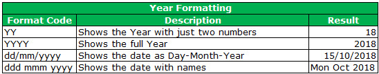
Format Codes for Year:
You can use the following two basic format codes to represent year values:
- yy – two-digit representation of year (e.g. 20 or 12)
- yyyy – four-digit representation of year (e.g. 2020 or 2012)
So, if you apply =TEXT(A2, yy) in our example dataset, it will return “18”.
If you apply =TEXT(A2, yyyy), then it will return “2018”.
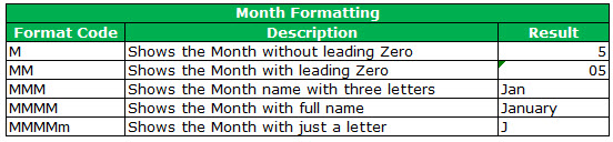
Format Codes for Month of the Year:
You can use the following four basic format codes to represent month values:
- m – one or two-digit representation of the month (eg; 8 or 12)
- mm – two-digit representation of the month (eg; 08 or 12)
- mmm – month abbreviated in three letters (eg: Aug or Dec)
- mmmm – month expressed with the full name (eg: August or December)
So, if you apply =TEXT(A2, m) in our example dataset, it will return “2”.
- If you apply =TEXT(A2, mm), then it will return “02”.
- If you apply =TEXT(A2, mmm), then it will return “Feb”.
- If you apply =TEXT(A2, mmmm), then it will return “February”.
Let us see how we can apply the TEXT function to our sample dataset to convert all the dates to different formats.
We will first see how to convert the dates in column A to the format shown in column B in the image below:

Below are the steps to change the date format and only get month and year using the TEXT function:
- Click on a blank cell where you want the new date format to be displayed (B2)
- Type the formula:
=TEXT(A2,”m/yy”)
- Press the Return key.
- This should display the original date in our required format. Copy this to the rest of the cells in the column by dragging down the fill handle or double-clicking on it.

- Copy this column’s formula results by pressing CTRL+C or Cmd+C (if you’re on a Mac).
- Right-click on the column and form the popup menu that appears, press Paste Values from the Paste Options.
- This will store the formula results as permanent values in the same column. Now you can go ahead and remove column A if you want to.


The format code that you put in the formula (at step 2) will vary according to the format you want your month and year to appear in. Here are the format codes along with the type of result you will get when applied to cell A2:
| Function | Result |
| =TEXT(A2, “mm/yy”) | 02/18 |
| =TEXT(A2, “mm-yy”) | 02-18 |
| =TEXT(A2, “mm-yyyy”) | 02-2018 |
| =TEXT(A2, “mmm, yyyy”) | Feb, 2018 |
| =TEXT(A2, “mmmm, yyyy”) | February, 2018 |

So you see, you can use the TEXT function to convert your dates to any format of your choice. All you need to do is change the format code according to your requirement.
Note: Using this formula, your date gets converted to a text format. If you want to convert it back to a date format, you need to use the Format Cells feature.
Also read: How to Convert Text to Date in Excel?
Convert Date to Month and Year using Number Formatting
Excel’s Format Cell feature is a versatile one that lets you perform different types of formatting through a single dialog box.
Here’s how you can convert the dates in our sample dataset to different formats.
- Select all the cells containing the dates that you want to convert (A2:A6).
- Right-click on your selection and select Format Cells from the popup menu that appears. Alternatively, you can select the dialog box launcher in the Number group under the Home tab.

- This will open the Format Cells dialog box. Click on the Number tab
- Under Category on the left side of the box, select the Date option.
- This will display a number of formatting options for date on the right side.
- Select the format that you want. For example, if you want to display the first date in the format “Feb-18”, then select the matching format option.

- If you don’t find an option for the format you want to use, then you can use the Custom option from the Category list on the left. This lets you convert the cell to a custom format.
- Look if your format is available among the date format codes under Type. If not, you can type in your format code in the input box just below Type. So, if you want to display the first month in the format “2/18”, then type “m/yy”.
- Click OK to close the Format Cells dialog box.


All your selected cells should now be formatted to your required format.

This method differs from the previous one (using the TEXT function) in four ways:
- With this method, you can perform the operation directly on the original cells.
- You can get your conversion done in one go. So you don’t need to have a separate cell to enter the formula, then paste by value and then delete the original cells (as you would need to if using the TEXT function).
- This method changes just the format of the original date, the underlying date, however, remains the same. So if you want to later recover the original date value (along with the day), you can easily access it. With the TEXT function method, however, the original date value is lost because the conversion changes the entire value of the date.
- The results you get from using this method are of type Date, rather than Text, so you can perform date operations on them directly without having to convert them.
These were three ways in which you can convert date to month and year in Excel. Using these you can convert your date to any format you need.
We hope you found our methods useful and that you will apply it to your own Excel data.
Other Excel tutorials you may like:
- How to Convert Decimal to Fraction in Excel
- How to Add Days to a Date in Excel
- How to Sort by Date in Excel (Single Column & Multiple Columns)
- How to Convert Serial Numbers to Date in Excel
- How to Convert Date to Day of Week in Excel
- How to Convert Month Number to Month Name in Excel
- How to Convert Days to Years in Excel (Simple Formulas)
- Convert Military Time to Standard Time in Excel (Formulas)
- Convert YYYYMMDD to MM/DD/YYYY in Excel
When we work in Excel often, we deal with numbers, text, and date format. Excel completely works on numbers. It will reflect the values based on the formatting you give. For example, the date and Time in excelTime is a time worksheet function in Excel that is used to calculate time based on the inputs provided by the user. The arguments can take the following formats: hours, minutes, and seconds.read more are stored as numbers and converted to readable values based on the formatting.
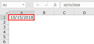
Look at the below example; the value in cell A1 is 43388. But, if we format it to date, it will show us the value as 15-10-2018.
You can download this Convert Date to Text Excel Template here – Convert Date to Text Excel Template

First, we must right-click on the cell and select the “Format Cells” option.

Then, we need to select the date option as shown below.
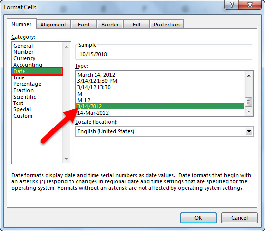
Now, the result will be as below.
So, Excel will reflect the numbers based on the formatting we apply.
Table of contents
- How to Convert Date to Text in Excel?
- Where can you Convert Date to Text in Excel?
- Example #1 – Convert Date to Text in Excel using “TEXT” Function
- Example #2 – Convert Date to Text in Excel using “TEXT” Function
- Example #3 – Convert Date to Text Using Text to Column Option
- Example #4 – Convert Date to Text in Excel using Formula
- Recommended Articles
Where can you Convert Date to Text in Excel?
Now, let us see some examples of converting dates to text in Excel.
When we need to convert Date to Text in ExcelYou can convert Date to Text in Excel through the most commonly used method, i.e., the text function or by using: Text-to-Column option, Copy Paste Method and VBA.
read more, we need to use the TEXT function in Excel. As mentioned, time and date in Excel are stored as numbers. However, sometimes we may require showing it as the text string. In such cases, we can use the TEXT function
- TEXT function consists of VALUE & FORMAT_TEXT.
- VALUE: It is the value we need to convert. It is simply the targeted cell. That could be a number, a reference cell that contains a number.
- FORMAT_TEXT: The format we need to provide to the cell, i.e., the targeted cell.
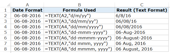
There are multiple date formats available in Excel. The below table will provide a better idea about the different formats and results.

Example #1 – Convert Date to Text in Excel using “TEXT” Function
We have the below values from cell A2 to A10 and convert them to the Date from B2 to B10.

To convert them to date format, in cell B2 write the below formula.
=TEXT(A3,”dd-mm-yyyy”)
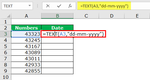
Press enter and drag the formula
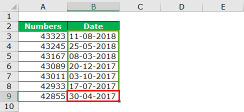
Example #2 – Convert Date to Text in Excel using “TEXT” Function
Take the below data and join the two columns (A2 & B2) together. For example, get the result as Shwetha Menon’s Birthdate is 14 Dec 2002.

Step 1:
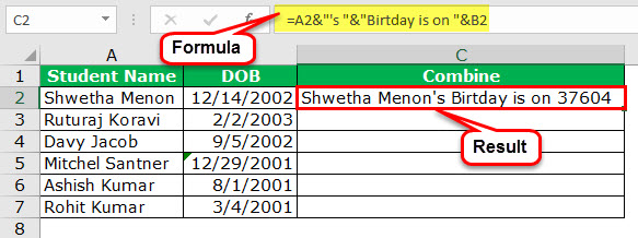
- We must go to cell C2 and apply the below concatenate code.

First, it will show the value as “Shwetha Menon’s Birthday is 37604.” It does not make sense to read it because the formula shows the date as numbers only. Therefore, we need to format the number and apply a date format.
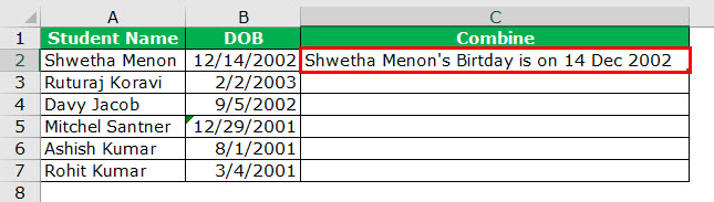
- Then, we must apply the TEXT function to get the correct format. In cell C2, we must use the below formula.

Result:

Note: We can apply different format styles shown in the early table to understand and get different results.

Example #3 – Convert Date to Text Using Text to Column Option
If we do not like formulas in Excel to convert the date to text format, we can use the TEXT TO COLUMN OPTION. Assume we have data from cells A2 to A8.

Now, we need to convert it into text format.
Step 1: We must first select the whole column that we want to convert.

Step 2: Then, we must go to Data > Convert Text to Columns Wizard in Excel.
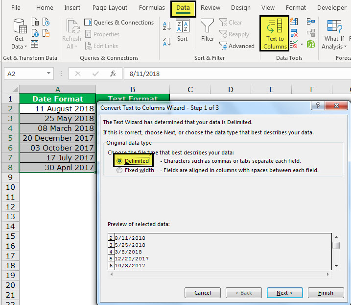
Step 3: We must ensure that the delimiter is selected and click the “Next” button.
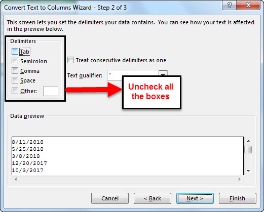
Step 4: Now, the pop-up below will open and uncheck all the boxes and click the “Next” button.
Step 5: We must select the “TEXT” option from the next dialog box. Then, we need to mention the destination cell as =$B$2 and click “Finish.”
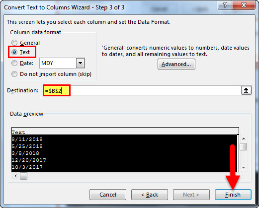
Step 6: As a result, it will instantly convert into text format..
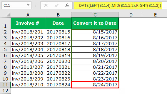
Example #4 – Convert Date to Text in Excel using Formula
We must use the formula method to convert the number to a date format. Assume we have the below data in our Excel file.
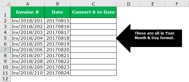
Formulas you need to know to convert them to YYYY-MM-DD are DATE, LEFT, RIGHT & MID functions. Moreover, the formula is.
Date: Date Function in ExcelThe date function in excel is a date and time function representing the number provided as arguments in a date and time code. The result displayed is in date format, but the arguments are supplied as integers.read more formats it into Year-Month-Day format.
![]()
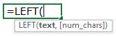
Left: LEFT Function in ExcelThe left function returns the number of characters from the start of the string. For example, if we use this function as =LEFT ( «ANAND»,2), the result will be AN.read more will take the first portion for year format. It takes 4 first 4 characters in year format.
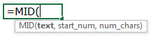
Mid: MID Function will take the middle part of the data for month format. It takes the middle 2 characters for a month format.
Right: RIGHT Function in ExcelRight function is a text function which gives the number of characters from the end from the string which is from right to left. For example, if we use this function as =RIGHT ( “ANAND”,2) this will give us ND as the result.read more will take the last part for Day format. Takes the last 2 characters for Day format.

Now, we must go ahead and apply the formula to get the date format.
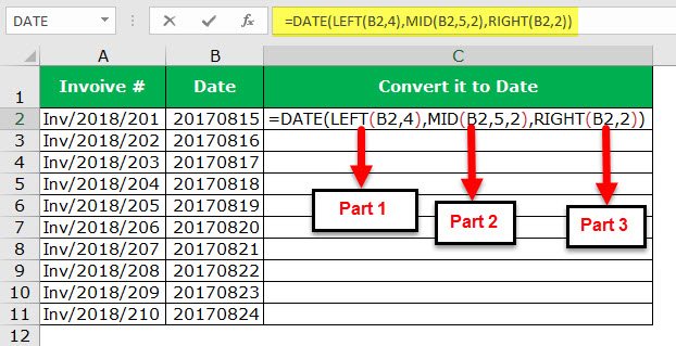
Now, let us elaborate on each part.
Part 1: LEFT (B2, 4) this means, in cell B2, take the first four characters. i.e., 2017
Part 2: MID (B2, 5, 2) this means, in cell B2, starting from 5th character, select two characters. i.e., 08.
Part 3: RIGHT (B2, 2) this means, in cell B2 from the right side, select two characters. i.e., 15
The Date function will combine all these and give you the value below. Next, drag and drop the formula for the remaining cells.
Recommended Articles
This article is a guide to Convert Date to Text in Excel. Here, we discuss converting date to text in Excel using three methods – 1) Text Function and 2) Text to Column Option 3) Formula Method, along with Excel examples and downloadable Excel templates. You may also look at these useful functions in Excel: –
- Excel Separate Text
- Add Text in Excel FormulaText in Excel Formula allows us to add text values to using the CONCATENATE function or the ampersand (&) symbol.read more
- Text to Columns in ExcelText to columns in excel is used to separate text in different columns based on some delimited or fixed width. This is done either by using a delimiter such as a comma, space or hyphen, or using fixed defined width to separate a text in the adjacent columns.read more
- MONTH Excel Function