
Содержание
- Replace a formula with its result
- Replace formulas with their calculated values
- Replace part of a formula with its calculated value
- Need more help?
- TEXT function
- Overview
- Download our examples
- Other format codes that are available
- Format codes by category
- Common scenario
- Frequently Asked Questions
Replace a formula with its result
You can convert the contents of a cell that contains a formula so that the calculated value replaces the formula. If you want to freeze only part of a formula, you can replace only the part you don’t want to recalculate. Replacing a formula with its result can be helpful if there are many or complex formulas in the workbook and you want to improve performance by creating static data.
You can convert formulas to their values on either a cell-by-cell basis or convert an entire range at once.
Important: Make sure you examine the impact of replacing a formula with its results, especially if the formulas reference other cells that contain formulas. It’s a good idea to make a copy of the workbook before replacing a formula with its results.
This article does not cover calculation options and methods. To find out how to turn on or off automatic recalculation for a worksheet, see Change formula recalculation, iteration, or precision.
Replace formulas with their calculated values
When you replace formulas with their values, Excel permanently removes the formulas. If you accidentally replace a formula with a value and want to restore the formula, click Undo  immediately after you enter or paste the value.
Select the cell or range of cells that contains the formulas.
If the formula is an array formula, select the range that contains the array formula.
How to select a range that contains the array formula
Click a cell in the array formula.
On the Home tab, in the Editing group, click Find & Select, and then click Go To.
Click Current array.
Click Copy  .
.
Click Paste  .
.
Click the arrow next to Paste Options  , and then click Values Only.
The following example shows a formula in cell D2 that multiplies cells A2, B2, and a discount derived from C2 to calculate an invoice amount for a sale. To copy the actual value instead of the formula from the cell to another worksheet or workbook, you can convert the formula in its cell to its value by doing the following:
Press F2 to edit the cell.
Press F9, and then press ENTER.
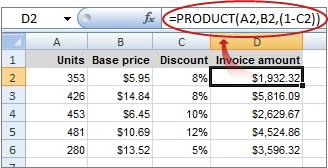
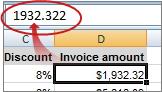
After you convert the cell from a formula to a value, the value appears as 1932.322 in the formula bar. Note that 1932.322 is the actual calculated value, and 1932.32 is the value displayed in the cell in a currency format.
Tip: When you are editing a cell that contains a formula, you can press F9 to permanently replace the formula with its calculated value.
Replace part of a formula with its calculated value
There may be times when you want to replace only a part of a formula with its calculated value. For example, you want to lock in the value that is used as a down payment for a car loan. That down payment was calculated based on a percentage of the borrower’s annual income. For the time being, that income amount won’t change, so you want to lock the down payment in a formula that calculates a payment based on various loan amounts.
When you replace a part of a formula with its value, that part of the formula cannot be restored.
Click the cell that contains the formula.
In the formula bar  , select the portion of the formula that you want to replace with its calculated value. When you select the part of the formula that you want to replace, make sure that you include the entire operand. For example, if you select a function, you must select the entire function name, the opening parenthesis, the arguments, and the closing parenthesis.
To calculate the selected portion, press F9.
To replace the selected portion of the formula with its calculated value, press ENTER.
In Excel for the web the results already appear in the workbook cell and the formula only appears in the formula bar .
Need more help?
You can always ask an expert in the Excel Tech Community or get support in the Answers community.
Источник
TEXT function
The TEXT function lets you change the way a number appears by applying formatting to it with format codes. It’s useful in situations where you want to display numbers in a more readable format, or you want to combine numbers with text or symbols.
Note: The TEXT function will convert numbers to text, which may make it difficult to reference in later calculations. It’s best to keep your original value in one cell, then use the TEXT function in another cell. Then, if you need to build other formulas, always reference the original value and not the TEXT function result.
The TEXT function syntax has the following arguments:
A numeric value that you want to be converted into text.
A text string that defines the formatting that you want to be applied to the supplied value.
Overview
In its simplest form, the TEXT function says:
=TEXT(Value you want to format, «Format code you want to apply»)
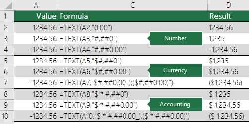
Here are some popular examples, which you can copy directly into Excel to experiment with on your own. Notice the format codes within quotation marks.
Currency with a thousands separator and 2 decimals, like $1,234.57. Note that Excel rounds the value to 2 decimal places.
Today’s date in MM/DD/YY format, like 03/14/12
Today’s day of the week, like Monday
Current time, like 1:29 PM
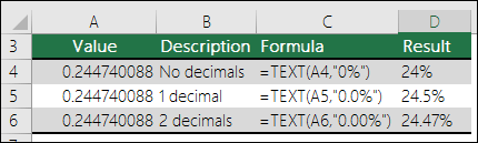
Percentage, like 28.5%
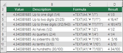
Fraction, like 4 1/3
Fraction, like 1/3. Note this uses the TRIM function to remove the leading space with a decimal value.
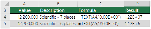
Scientific notation, like 1.22E+07
Add leading zeros (0), like 0001234
Note: Although you can use the TEXT function to change formatting, it’s not the only way. You can change the format without a formula by pressing CTRL+1 (or  +1 on the Mac), then pick the format you want from the Format Cells > Number dialog.
Download our examples
You can download an example workbook with all of the TEXT function examples you’ll find in this article, plus some extras. You can follow along, or create your own TEXT function format codes.
Other format codes that are available
You can use the Format Cells dialog to find the other available format codes:
Press Ctrl+1 ( +1 on the Mac) to bring up the Format Cells dialog.
Select the format you want from the Number tab.
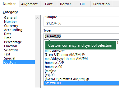
Select the Custom option,
The format code you want is now shown in the Type box. In this case, select everything from the Type box except the semicolon (;) and @ symbol. In the example below, we selected and copied just mm/dd/yy.
Press Ctrl+C to copy the format code, then press Cancel to dismiss the Format Cells dialog.
Now, all you need to do is press Ctrl+V to paste the format code into your TEXT formula, like: =TEXT(B2,» mm/dd/yy«). Make sure that you paste the format code within quotes («format code»), otherwise Excel will throw an error message.
 Cells > Number > Custom dialog to have Excel create format strings for you.» loading=»lazy»>
Format codes by category
Following are some examples of how you can apply different number formats to your values by using the Format Cells dialog, then use the Custom option to copy those format codes to your TEXT function.
Why does Excel delete my leading 0’s?
Excel is trained to look for numbers being entered in cells, not numbers that look like text, like part numbers or SKU’s. To retain leading zeros, format the input range as Text before you paste or enter values. Select the column, or range where you’ll be putting the values, then use CTRL+1 to bring up the Format > Cells dialog and on the Number tab select Text. Now Excel will keep your leading 0’s.
If you’ve already entered data and Excel has removed your leading 0’s, you can use the TEXT function to add them back. You can reference the top cell with the values and use =TEXT(value,»00000″), where the number of 0’s in the formula represents the total number of characters you want, then copy and paste to the rest of your range.
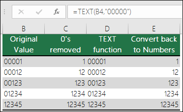
If for some reason you need to convert text values back to numbers you can multiply by 1, like =D4*1, or use the double-unary operator (—), like =—D4.
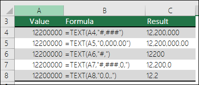
Excel separates thousands by commas if the format contains a comma (,) that is enclosed by number signs (#) or by zeros. For example, if the format string is «#,###», Excel displays the number 12200000 as 12,200,000.
A comma that follows a digit placeholder scales the number by 1,000. For example, if the format string is «#,###.0,», Excel displays the number 12200000 as 12,200.0.
The thousands separator is dependent on your regional settings. In the US it’s a comma, but in other locales it might be a period (.).
The thousands separator is available for the number, currency and accounting formats.
Following are examples of standard number (thousands separator and decimals only), currency and accounting formats. Currency format allows you to insert the currency symbol of your choice and aligns it next to your value, while accounting format will align the currency symbol to the left of the cell and the value to the right. Note the difference between the currency and accounting format codes below, where accounting uses an asterisk (*) to create separation between the symbol and the value.
To find the format code for a currency symbol, first press Ctrl+1 (or +1 on the Mac), select the format you want, then choose a symbol from the Symbol drop-down:
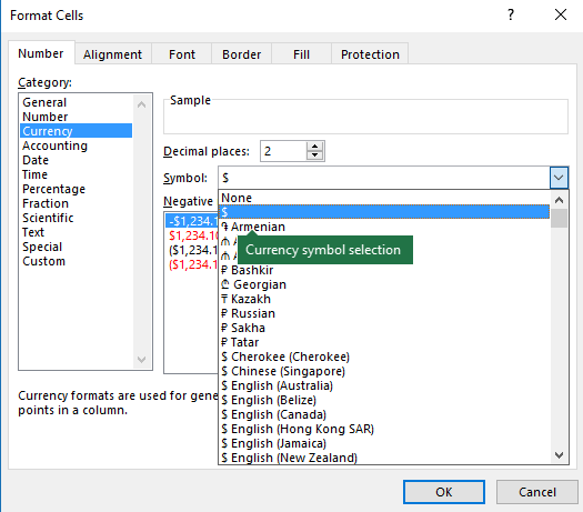
Then click Custom on the left from the Category section, and copy the format code, including the currency symbol.
Note: The TEXT function does not support color formatting, so if you copy a number format code from the Format Cells dialog that includes a color, like this: $#,##0.00_); [Red]($#,##0.00), the TEXT function will accept the format code, but it won’t display the color.
You can alter the way a date displays by using a mix of «M» for month, «D» for days, and «Y» for years.
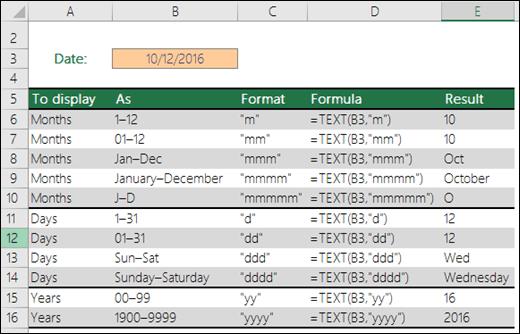
Format codes in the TEXT function aren’t case sensitive, so you can use either «M» or «m», «D» or «d», «Y» or «y».

If you share Excel files and reports with users from different countries, then you might want to give them a report in their language. Excel MVP, Mynda Treacy has a great solution in this Excel Dates Displayed in Different Languages article. It also includes a sample workbook you can download.
You can alter the way time displays by using a mix of «H» for hours, «M» for minutes, or «S» for seconds, and «AM/PM» for a 12-hour clock.
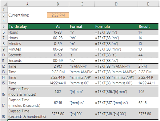
If you leave out the «AM/PM» or «A/P», then time will display based on a 24-hour clock.
Format codes in the TEXT function aren’t case sensitive, so you can use either «H» or «h», «M» or «m», «S» or «s», «AM/PM» or «am/pm».
You can alter the way decimal values display with percentage (%) formats.
You can alter the way decimal values display with fraction (?/?) formats.
Scientific notation is a way of displaying numbers in terms of a decimal between 1 and 10, multiplied by a power of 10. It is often used to shorten the way that large numbers display.
Excel provides 4 special formats:
Zip Code — «00000»
Zip Code + 4 — «00000-0000»
Social Security Number — «000-00-0000»
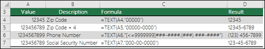
Special formats will be different depending on locale, but if there aren’t any special formats for your locale, or if these don’t meet your needs then you can create your own through the Format Cells > Custom dialog.
Common scenario
The TEXT function is rarely used by itself, and is most often used in conjunction with something else. Let’s say you want to combine text and a number value, like “Report Printed on: 03/14/12”, or “Weekly Revenue: $66,348.72”. You could type that into Excel manually, but that defeats the purpose of having Excel do it for you. Unfortunately, when you combine text and formatted numbers, like dates, times, currency, etc., Excel doesn’t know how you want to display them, so it drops the number formatting. This is where the TEXT function is invaluable, because it allows you to force Excel to format the values the way you want by using a format code, like «MM/DD/YY» for date format.
In the following example, you’ll see what happens if you try to join text and a number without using the TEXT function. In this case, we’re using the ampersand ( &) to concatenate a text string, a space (» «), and a value with =A2&» «&B2.
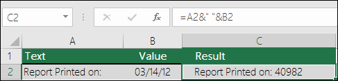
As you can see, Excel removed the formatting from the date in cell B2. In the next example, you’ll see how the TEXT function lets you apply the format you want.
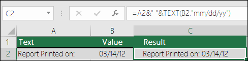
Our updated formula is:
Cell C2: =A2&» «&TEXT(B2,»mm/dd/yy») — Date format
Frequently Asked Questions
Unfortunately, you can’t do that with the TEXT function, you need to use Visual Basic for Applications (VBA) code. The following link has a method: How to convert a numeric value into English words in Excel
Yes, you can use the UPPER, LOWER and PROPER functions. For example, =UPPER(«hello») would return «HELLO».
Yes, but it takes a few steps. First, select the cell or cells where you want this to happen and use Ctrl+1 to bring up the Format > Cells dialog, then Alignment > Text control > check the Wrap Text option. Next, adjust your completed TEXT function to include the ASCII function CHAR(10) where you want the line break. You might need to adjust your column width depending on how the final result aligns.
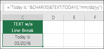
In this case, we used: =»Today is: «&CHAR(10)&TEXT(TODAY(),»mm/dd/yy»)
This is called Scientific Notation, and Excel will automatically convert numbers longer than 12 digits if a cell(s) is formatted as General, and 15 digits if a cell(s) is formatted as a Number. If you need to enter long numeric strings, but don’t want them converted, then format the cells in question as Text before you input or paste your values into Excel.
If you share Excel files and reports with users from different countries, then you might want to give them a report in their language. Excel MVP, Mynda Treacy has a great solution in this Excel Dates Displayed in Different Languages article. It also includes a sample workbook you can download.
Источник
Содержание
- 1 Преобразование формулы в текст в Excel
- 2 Функция Ф.ТЕКСТ в Excel
- 3 Замечания
- 4 Пользовательская функция (UDF)
- 5 Процедура вставки текста около формулы
- 6 Способ 1: использование амперсанда
- 7 Способ 2: применение функции СЦЕПИТЬ
- 7.1 Помогла ли вам эта статья?
Познакомимся с вариантами преобразования формулы Excel в текст (в результате получается не значение ячейки, а формульное выражение в текстовом виде, например, «=A1+A2», «=СЕГОДНЯ()» и т.д.).
Возникают ситуации когда необходимо отобразить в ячейке не значение формульного выражения, а именно ее текстовую запись.
С помощью режима отображения формул мы можем увидеть все формульные выражения листа и книги в текстовом виде, однако если мы хотим показать формулу не для всех, а для каких-то конкретных ячеек, то такой вариант не подходит.
Однако вне зависимости от целей преобразования нам понадобится способ извлечь из ячейки строку с формулой.
Начнем с более простого варианта, а именно предположим, что нам нужно преобразовать формулу в текст в самой ячейке (т.е. заменить значение на текстовую запись). Тогда в этом случае есть несколько способов преобразования:
- Поменять формат ячейки на текстовый, а затем произвести вычисление формулы;При этом для каждой ячейки нужно будет вручную производить изменение.
- Добавить апостроф (символ «‘») перед знаком равно (символ «=») в формульном выражении.В данном варианте подставить апостроф можно как вручную, так и через замену («=» на «‘=» с помощью инструмента «Найти и заменить»).

Теперь перейдем к более общему случаю и рассмотрим 2 основных варианта перевода формулы в текст (т.е. получить текстовую запись):
- Функция Ф.ТЕКСТ (доступна начиная с версии Excel 2013);
- Пользовательская функция (UDF).
Первый способ позволит нам перевести формулу в текст стандартными средствами в Excel, а во втором способе мы напишем пользовательскую функцию, которая будет выполнять аналогичные по функционалу преобразования (что и в первом способе) с небольшими видоизменениями.
Давайте подробнее остановимся на каждом из них.
Функция Ф.ТЕКСТ в Excel
Начиная с версии Excel 2013 для применения доступна функция Ф.ТЕКСТ (FORMULATEXT в английской версии):
Ф.ТЕКСТ(ссылка)
Возвращает формулу в виде строки.
- Ссылка (обязательный аргумент) — ссылка на ячейку или диапазон ячеек.
Перейдем к примерам. Применим Ф.ТЕКСТ, в качестве аргумента укажем ссылку на произвольную ячейку, где содержится какое-либо формульное выражение:

При этом в зависимости от выбранного у вас параметра отображения стиля ссылок (A1 или R1C1) формула автоматически будет подстраиваться под формат записи:

Замечания
При работе с данной функцией есть несколько важных особенностей, на которые необходимо обратить внимание:
- Аргумент «Ссылка» может ссылаться на другие листы и книги;
- Если аргумент «Ссылка» не содержит формульное выражение или содержит ссылку на закрытую книгу, то в результате будет возвращено значение ошибки.
Пользовательская функция (UDF)
При использовании версии Excel 2010 или более ранней, стандартными инструментами Excel воспользоваться уже не получится.
Однако данную проблему мы можем решить с помощью создания пользовательской функции (UDF), которая позволит преобразовать формулу в текст в различных вариантах записи в зависимости от стиля ссылок.
Перейдем в редактор Visual Basic (сочетание клавиш Alt + F11), вставляем новый модуль и добавляем следующий код:
|
Public Function FText(myRange As Range) As String FText = myRange.FormulaLocal End Function |
Как обычно, к новой функции мы можем обратиться либо через мастер функций (выбрав ее из категории Определенные пользователем), либо ввести формульное выражение в пустую ячейку:

Как видим результат работы пользовательской функции FText получился точно таким же, как и у стандартной Ф.ТЕКСТ.
В данном примере мы использовали свойство диапазона FormulaLocal, которое позволяет преобразовать формульное выражение со стилем ссылок A1, однако в зависимости от предпочтений стиль записи можно изменить, а именно поменять свойство FormulaLocal на один из следующих вариантов:
- Formula — формат A1 (англоязычная формула);
- FormulaR1C1 — формат R1C1 (англоязычная);
- FormulaLocal — формат A1 (неанглоязычная/местная);
- FormulaR1C1Local — формат R1C1 (неанглоязычная/местная).
Выбираем необходимый формат записи, корректируем код FText в VBA и на выходе получаем итоговое преобразование:

Удачи вам и до скорых встреч на страницах блога Tutorexcel.ru!

Довольно часто при работе в Excel существует необходимость рядом с результатом вычисления формулы вставить поясняющий текст, который облегчает понимание этих данных. Конечно, можно выделить для пояснений отдельный столбец, но не во всех случаях добавление дополнительных элементов является рациональным. Впрочем, в Экселе имеются способы поместить формулу и текст в одну ячейку вместе. Давайте разберемся, как это можно сделать при помощи различных вариантов.
Процедура вставки текста около формулы
Если просто попробовать вставить текст в одну ячейку с функцией, то при такой попытке Excel выдаст сообщение об ошибке в формуле и не позволит совершить такую вставку. Но существует два способа все-таки вставить текст рядом с формульным выражением. Первый из них заключается в применении амперсанда, а второй – в использовании функции СЦЕПИТЬ.

Способ 1: использование амперсанда
Самый простой способ решить данную задачу – это применить символ амперсанда (&). Данный знак производит логическое отделение данных, которые содержит формула, от текстового выражения. Давайте посмотрим, как можно применить указанный способ на практике.
У нас имеется небольшая таблица, в которой в двух столбцах указаны постоянные и переменные затраты предприятия. В третьем столбце находится простая формула сложения, которая суммирует их и выводит общим итогом. Нам требуется в ту же ячейку, где отображается общая сумма затрат добавить после формулы поясняющее слово «рублей».

- Активируем ячейку, содержащую формульное выражение. Для этого либо производим по ней двойной щелчок левой кнопкой мыши, либо выделяем и жмем на функциональную клавишу F2. Также можно просто выделить ячейку, а потом поместить курсор в строку формул.
- Сразу после формулы ставим знак амперсанд (&). Далее в кавычках записываем слово «рублей». При этом кавычки не будут отображаться в ячейке после числа выводимого формулой. Они просто служат указателем для программы, что это текст. Для того, чтобы вывести результат в ячейку, щелкаем по кнопке Enter на клавиатуре.
- Как видим, после этого действия, вслед за числом, которое выводит формула, находится пояснительная надпись «рублей». Но у этого варианта есть один видимый недостаток: число и текстовое пояснение слились воедино без пробела.

При этом, если мы попытаемся поставить пробел вручную, то это ничего не даст. Как только будет нажата кнопка Enter, результат снова «склеится».
- Но из сложившейся ситуации все-таки существует выход. Снова активируем ячейку, которая содержит формульное и текстовое выражения. Сразу после амперсанда открываем кавычки, затем устанавливаем пробел, кликнув по соответствующей клавише на клавиатуре, и закрываем кавычки. После этого снова ставим знак амперсанда (&). Затем щелкаем по клавише Enter.
- Как видим, теперь результат вычисления формулы и текстовое выражение разделены пробелом.


Естественно, что все указанные действия проделывать не обязательно. Мы просто показали, что при обычном введении без второго амперсанда и кавычек с пробелом, формульные и текстовые данные сольются. Вы же можете установить правильный пробел ещё при выполнении второго пункта данного руководства.
При написании текста перед формулой придерживаемся следующего синтаксиса. Сразу после знака «=» открываем кавычки и записываем текст. После этого закрываем кавычки. Ставим знак амперсанда. Затем, в случае если нужно внести пробел, открываем кавычки, ставим пробел и закрываем кавычки. Щелкаем по клавише Enter.

Для записи текста вместе с функцией, а не с обычной формулой, все действия точно такие же, как были описаны выше.

Текст также можно указывать в виде ссылки на ячейку, в которой он расположен. В этом случае, алгоритм действий остается прежним, только сами координаты ячейки в кавычки брать не нужно.

Способ 2: применение функции СЦЕПИТЬ
Также для вставки текста вместе с результатом подсчета формулы можно использовать функцию СЦЕПИТЬ. Данный оператор предназначен для того, чтобы соединять в одной ячейке значения, выводимые в нескольких элементах листа. Он относится к категории текстовых функций. Его синтаксис следующий:
=СЦЕПИТЬ(текст1;текст2;…)
Всего у этого оператора может быть от 1 до 255 аргументов. Каждый из них представляет либо текст (включая цифры и любые другие символы), либо ссылки на ячейки, которые его содержат.
Посмотрим, как работает данная функция на практике. Для примера возьмем все ту же таблицу, только добавим в неё ещё один столбец «Общая сумма затрат» с пустой ячейкой.
- Выделяем пустую ячейку столбца «Общая сумма затрат». Щелкаем по пиктограмме «Вставить функцию», расположенную слева от строки формул.
- Производится активация Мастера функций. Перемещаемся в категорию «Текстовые». Далее выделяем наименование «СЦЕПИТЬ» и жмем на кнопку «OK».
- Запускается окошко аргументов оператора СЦЕПИТЬ. Данное окно состоит из полей под наименованием «Текст». Их количество достигает 255, но для нашего примера понадобится всего три поля. В первом мы разместим текст, во втором – ссылку на ячейку, в которой содержится формула, и в третьем опять разместим текст.
Устанавливаем курсор в поле «Текст1». Вписываем туда слово «Итого». Писать текстовые выражения можно без кавычек, так как программа проставит их сама.
Потом переходим в поле «Текст2». Устанавливаем туда курсор. Нам нужно тут указать то значение, которое выводит формула, а значит, следует дать ссылку на ячейку, её содержащую. Это можно сделать, просто вписав адрес вручную, но лучше установить курсор в поле и кликнуть по ячейке, содержащей формулу на листе. Адрес отобразится в окошке аргументов автоматически.
В поле «Текст3» вписываем слово «рублей».
После этого щелкаем по кнопке «OK».
- Результат выведен в предварительно выделенную ячейку, но, как видим, как и в предыдущем способе, все значения записаны слитно без пробелов.
- Для того, чтобы решить данную проблему, снова выделяем ячейку, содержащую оператор СЦЕПИТЬ и переходим в строку формул. Там после каждого аргумента, то есть, после каждой точки с запятой добавляем следующее выражение:
" ";Между кавычками должен находиться пробел. В целом в строке функций должно отобразиться следующее выражение:
=СЦЕПИТЬ("Итого";" ";D2;" ";"рублей")Щелкаем по клавише ENTER. Теперь наши значения разделены пробелами.
- При желании можно спрятать первый столбец «Общая сумма затрат» с исходной формулой, чтобы он не занимал лишнее место на листе. Просто удалить его не получится, так как это нарушит функцию СЦЕПИТЬ, но убрать элемент вполне можно. Кликаем левой кнопкой мыши по сектору панели координат того столбца, который следует скрыть. После этого весь столбец выделяется. Щелкаем по выделению правой кнопкой мыши. Запускается контекстное меню. Выбираем в нем пункт «Скрыть».
- После этого, как видим, ненужный нам столбец скрыт, но при этом данные в ячейке, в которой расположена функция СЦЕПИТЬ отображаются корректно.
Читайте также: Функция СЦЕПИТЬ в Экселе
Как скрыть столбцы в Экселе
Таким образом, можно сказать, что существуют два способа вписать в одну ячейку формулу и текст: при помощи амперсанда и функции СЦЕПИТЬ. Первый вариант проще и для многих пользователей удобнее. Но, тем не менее, в определенных обстоятельствах, например при обработке сложных формул, лучше пользоваться оператором СЦЕПИТЬ.
Мы рады, что смогли помочь Вам в решении проблемы.
Задайте свой вопрос в комментариях, подробно расписав суть проблемы. Наши специалисты постараются ответить максимально быстро.
Помогла ли вам эта статья?
Да Нет
| Здесь можно получить ответы на вопросы по Microsoft Excel | 58510 | 478918 |
8 Ноя 2018 19:00:01 |
|
| 44519 | 357828 |
29 Янв 2017 17:28:40 |
||
| Лучшие избранные темы с основного форума | 14 | 80 |
28 Июн 2018 15:25:11 |
|
| Если вы — счастливый обладатель Mac 😉 | 219 | 1065 |
25 Окт 2018 09:26:29 |
|
| Раздел для размещения платных вопросов, проектов и задач и поиска исполнителей для них. | 2138 | 13647 |
8 Ноя 2018 16:58:12 |
|
| Если Вы скачали или приобрели надстройку PLEX для Microsoft Excel и у Вас есть вопросы или пожелания — Вам сюда. | 316 | 1615 |
6 Ноя 2018 20:49:07 |
|
| 820 | 11946 |
8 Ноя 2018 15:55:43 |
||
| Обсуждение функционала, правил и т.д. | 270 | 3481 |
30 Окт 2018 15:01:36 |
|
Сейчас на форуме (гостей: 1220, пользователей: 17, из них скрытых: 3) , , , , , , , , , , , , ,
Сегодня отмечают день рождения (41), (32), (3), (39), (38), (33), (28)
Всего зарегистрированных пользователей: 83822
Приняло участие в обсуждении: 32154
Всего тем: 106806
Replace formulas with their calculated values
When you replace formulas with their values, Excel permanently removes the formulas. If you accidentally replace a formula with a value and want to restore the formula, click Undo immediately after you enter or paste the value.
-
Select the cell or range of cells that contains the formulas.
If the formula is an array formula, select the range that contains the array formula.
How to select a range that contains the array formula
-
Click a cell in the array formula.
-
On the Home tab, in the Editing group, click Find & Select, and then click Go To.
-
Click Special.
-
Click Current array.
-
-
Click Copy
 .
. -
Click Paste
. -
Click the arrow next to Paste Options
, and then click Values Only.
The following example shows a formula in cell D2 that multiplies cells A2, B2, and a discount derived from C2 to calculate an invoice amount for a sale. To copy the actual value instead of the formula from the cell to another worksheet or workbook, you can convert the formula in its cell to its value by doing the following:
-
Press F2 to edit the cell.
-
Press F9, and then press ENTER.
After you convert the cell from a formula to a value, the value appears as 1932.322 in the formula bar. Note that 1932.322 is the actual calculated value, and 1932.32 is the value displayed in the cell in a currency format.
Tip: When you are editing a cell that contains a formula, you can press F9 to permanently replace the formula with its calculated value.
Replace part of a formula with its calculated value
There may be times when you want to replace only a part of a formula with its calculated value. For example, you want to lock in the value that is used as a down payment for a car loan. That down payment was calculated based on a percentage of the borrower’s annual income. For the time being, that income amount won’t change, so you want to lock the down payment in a formula that calculates a payment based on various loan amounts.
When you replace a part of a formula with its value, that part of the formula cannot be restored.
-
Click the cell that contains the formula.
-
In the formula bar
, select the portion of the formula that you want to replace with its calculated value. When you select the part of the formula that you want to replace, make sure that you include the entire operand. For example, if you select a function, you must select the entire function name, the opening parenthesis, the arguments, and the closing parenthesis. -
To calculate the selected portion, press F9.
-
To replace the selected portion of the formula with its calculated value, press ENTER.
In Excel for the web the results already appear in the workbook cell and the formula only appears in the formula bar .
Generally, in Excel, when we type «=» before any string, it will be treated as a formula. But sometimes there can be some strings that are needed to be entered on a sheet that start with the «=» sign. And also, sometimes we needed to convert the existing formulas to strings.
In this tutorial, we will learn how to convert formulas to text strings in Excel. We can complete this process by using the find and replace function in Excel. In this process, all the formulas present in the sheet will be converted into strings.
Converting a Formula to Text String in Excel
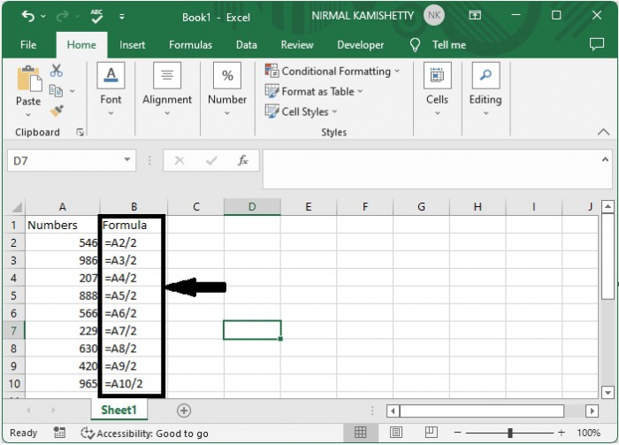
Here we will insert a space before the equal symbol to complete the task. Let’s take a look at a simple procedure for converting formulas to text strings in Excel. We can complete it by using the find and replace function in Excel.
Step 1
Let us consider any Excel sheet where the data in the sheet is similar to the below image.
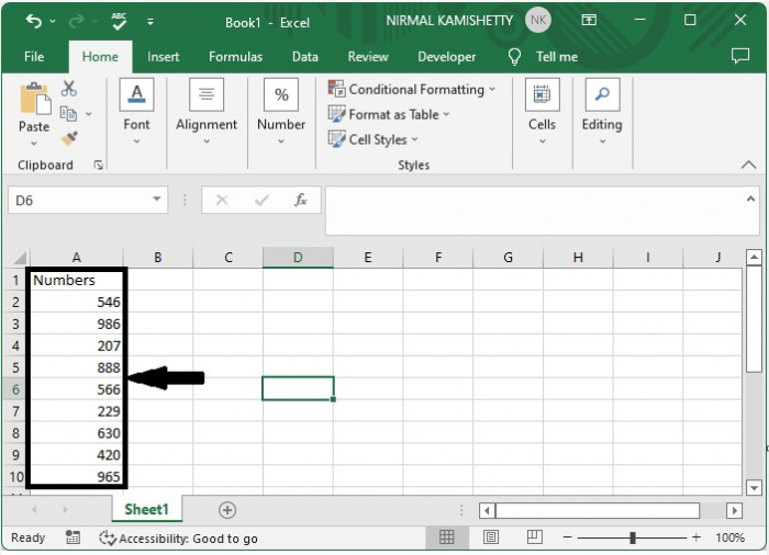
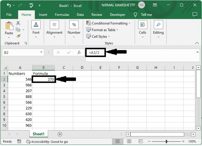
To apply the formula Click on any empty cell, in our case cell B2, and enter the formula as «=A2/2» and click Enter, as shown in the below image.
Step 2
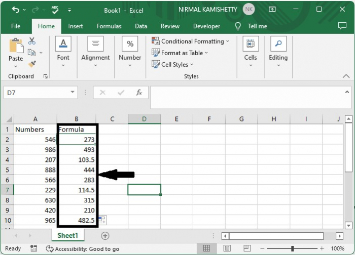
To apply the formula to all the cells drag down from the first result using the auto fill handle and it will look similar to screenshot given below.
Step 3
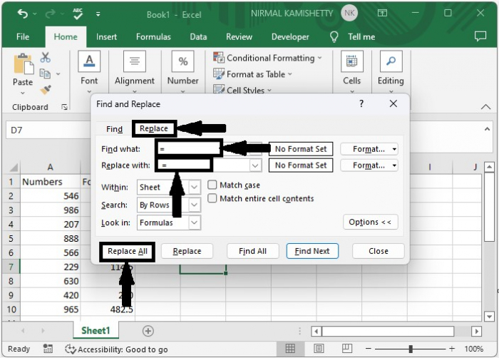
To convert the formula to a string, use the command CTRL + F to open the find and replace menu, then click on replace, enter «=» in find what and » =» in replace with, and click on replace all as shown in the below image.
CTRL + F > Replace > «=» > » =» > Replace all
And our final output will look similar to the screenshot given below.
Conclusion
In this tutorial, we used a simple example to demonstrate how you can convert a formula to a text string in Excel.
If you’ve ever been frustrated by the fact that there is no way to convert formula to text string in excel, this is the article for you. Excel has been around for years, and it’s still going strong. One of the things that makes it so popular is that it’s easy to use. But when you need to get more advanced or want to do something outside of the box, it can be tough. There are some ways to make this easier on yourself though—for example, if you’re trying to convert a formula into a text string in Excel, here are some ways you can do it.
How To Convert Formula To Text String In Excel using Paste Special?
For those of us who work in Excel and use formulas, it’s a pain to have to go back and convert everything from formulas to text strings. Luckily, there’s a way to do this with a simple paste special trick.
This method works best with versions 2016/2016/mac/online.
1. In a worksheet, select the cell range containing formulas you want to convert to text.
2. Then, go to the cell where you want to paste the converted formulas.
3. Right-click and choose Paste Special from the shortcut menu that appears. In the Paste Special dialog box, click on Paste as Values.
4. The converted formulas will be pasted immediately into the worksheet.
How To Convert Formula To Text String In Excel using Keyboard Shortcut?
You can convert formula to text string in Excel with an easy keyboard shortcut. You can use the keyboard shortcut to quickly convert any formula into a text string, which means that it will show up as text rather than as a formula. This is useful if you want to see what your formula looks like when it’s not being evaluated.
This method works best with versions 2016/2016/mac/online.
1. To convert formulas to values, select the cells you want to change and copy them.
2. Then paste the copied cells as values by pressing ALT + ESV.
How To Convert Formula To Text String In Excel using Paste Options?
The Paste Options feature allows you to convert a cell’s formula to text or value. This is useful if you have a long formula and need to save it as plain text.
This method works best with versions 2016/2016/mac/online.
1. When you copy and paste a range of cells, an icon appears in the lower right corner. It remains there until you interact with the spreadsheet.
2. These options allow you to change the pasted cells into values only. The Paste Special command is accessed by clicking on the Paste Options icon or pressing Ctrl.
3. When you open the menu, you can then either click on the Values icon or press V to change the range into values only.
Did you learn about how to convert formula to text string in excel? You can follow WPS Academy to learn more features of Word Document, Excel Spreadsheets and PowerPoint Slides.
You can also download WPS Office to edit the word documents, excel, PowerPoint for free of cost. Download now! And get an easy and enjoyable working experience.