
The IF function allows you to make a logical comparison between a value and what you expect by testing for a condition and returning a result if that condition is True or False.
-
=IF(Something is True, then do something, otherwise do something else)
But what if you need to test multiple conditions, where let’s say all conditions need to be True or False (AND), or only one condition needs to be True or False (OR), or if you want to check if a condition does NOT meet your criteria? All 3 functions can be used on their own, but it’s much more common to see them paired with IF functions.
Use the IF function along with AND, OR and NOT to perform multiple evaluations if conditions are True or False.
Syntax
-
IF(AND()) — IF(AND(logical1, [logical2], …), value_if_true, [value_if_false]))
-
IF(OR()) — IF(OR(logical1, [logical2], …), value_if_true, [value_if_false]))
-
IF(NOT()) — IF(NOT(logical1), value_if_true, [value_if_false]))
|
Argument name |
Description |
|
|
logical_test (required) |
The condition you want to test. |
|
|
value_if_true (required) |
The value that you want returned if the result of logical_test is TRUE. |
|
|
value_if_false (optional) |
The value that you want returned if the result of logical_test is FALSE. |
|
Here are overviews of how to structure AND, OR and NOT functions individually. When you combine each one of them with an IF statement, they read like this:
-
AND – =IF(AND(Something is True, Something else is True), Value if True, Value if False)
-
OR – =IF(OR(Something is True, Something else is True), Value if True, Value if False)
-
NOT – =IF(NOT(Something is True), Value if True, Value if False)
Examples
Following are examples of some common nested IF(AND()), IF(OR()) and IF(NOT()) statements. The AND and OR functions can support up to 255 individual conditions, but it’s not good practice to use more than a few because complex, nested formulas can get very difficult to build, test and maintain. The NOT function only takes one condition.

Here are the formulas spelled out according to their logic:
|
Formula |
Description |
|---|---|
|
=IF(AND(A2>0,B2<100),TRUE, FALSE) |
IF A2 (25) is greater than 0, AND B2 (75) is less than 100, then return TRUE, otherwise return FALSE. In this case both conditions are true, so TRUE is returned. |
|
=IF(AND(A3=»Red»,B3=»Green»),TRUE,FALSE) |
If A3 (“Blue”) = “Red”, AND B3 (“Green”) equals “Green” then return TRUE, otherwise return FALSE. In this case only the first condition is true, so FALSE is returned. |
|
=IF(OR(A4>0,B4<50),TRUE, FALSE) |
IF A4 (25) is greater than 0, OR B4 (75) is less than 50, then return TRUE, otherwise return FALSE. In this case, only the first condition is TRUE, but since OR only requires one argument to be true the formula returns TRUE. |
|
=IF(OR(A5=»Red»,B5=»Green»),TRUE,FALSE) |
IF A5 (“Blue”) equals “Red”, OR B5 (“Green”) equals “Green” then return TRUE, otherwise return FALSE. In this case, the second argument is True, so the formula returns TRUE. |
|
=IF(NOT(A6>50),TRUE,FALSE) |
IF A6 (25) is NOT greater than 50, then return TRUE, otherwise return FALSE. In this case 25 is not greater than 50, so the formula returns TRUE. |
|
=IF(NOT(A7=»Red»),TRUE,FALSE) |
IF A7 (“Blue”) is NOT equal to “Red”, then return TRUE, otherwise return FALSE. |
Note that all of the examples have a closing parenthesis after their respective conditions are entered. The remaining True/False arguments are then left as part of the outer IF statement. You can also substitute Text or Numeric values for the TRUE/FALSE values to be returned in the examples.
Here are some examples of using AND, OR and NOT to evaluate dates.

Here are the formulas spelled out according to their logic:
|
Formula |
Description |
|---|---|
|
=IF(A2>B2,TRUE,FALSE) |
IF A2 is greater than B2, return TRUE, otherwise return FALSE. 03/12/14 is greater than 01/01/14, so the formula returns TRUE. |
|
=IF(AND(A3>B2,A3<C2),TRUE,FALSE) |
IF A3 is greater than B2 AND A3 is less than C2, return TRUE, otherwise return FALSE. In this case both arguments are true, so the formula returns TRUE. |
|
=IF(OR(A4>B2,A4<B2+60),TRUE,FALSE) |
IF A4 is greater than B2 OR A4 is less than B2 + 60, return TRUE, otherwise return FALSE. In this case the first argument is true, but the second is false. Since OR only needs one of the arguments to be true, the formula returns TRUE. If you use the Evaluate Formula Wizard from the Formula tab you’ll see how Excel evaluates the formula. |
|
=IF(NOT(A5>B2),TRUE,FALSE) |
IF A5 is not greater than B2, then return TRUE, otherwise return FALSE. In this case, A5 is greater than B2, so the formula returns FALSE. |

Using AND, OR and NOT with Conditional Formatting
You can also use AND, OR and NOT to set Conditional Formatting criteria with the formula option. When you do this you can omit the IF function and use AND, OR and NOT on their own.
From the Home tab, click Conditional Formatting > New Rule. Next, select the “Use a formula to determine which cells to format” option, enter your formula and apply the format of your choice.

Using the earlier Dates example, here is what the formulas would be.

|
Formula |
Description |
|---|---|
|
=A2>B2 |
If A2 is greater than B2, format the cell, otherwise do nothing. |
|
=AND(A3>B2,A3<C2) |
If A3 is greater than B2 AND A3 is less than C2, format the cell, otherwise do nothing. |
|
=OR(A4>B2,A4<B2+60) |
If A4 is greater than B2 OR A4 is less than B2 plus 60 (days), then format the cell, otherwise do nothing. |
|
=NOT(A5>B2) |
If A5 is NOT greater than B2, format the cell, otherwise do nothing. In this case A5 is greater than B2, so the result will return FALSE. If you were to change the formula to =NOT(B2>A5) it would return TRUE and the cell would be formatted. |
Note: A common error is to enter your formula into Conditional Formatting without the equals sign (=). If you do this you’ll see that the Conditional Formatting dialog will add the equals sign and quotes to the formula — =»OR(A4>B2,A4<B2+60)», so you’ll need to remove the quotes before the formula will respond properly.
Need more help?

See also
You can always ask an expert in the Excel Tech Community or get support in the Answers community.
Learn how to use nested functions in a formula
IF function
AND function
OR function
NOT function
Overview of formulas in Excel
How to avoid broken formulas
Detect errors in formulas
Keyboard shortcuts in Excel
Logical functions (reference)
Excel functions (alphabetical)
Excel functions (by category)
Conditional formatting is used to highlight the cells where a given condition is met. However, if we want to highlight the cells that meet multiple conditions, then conditional formatting with AND function is used.
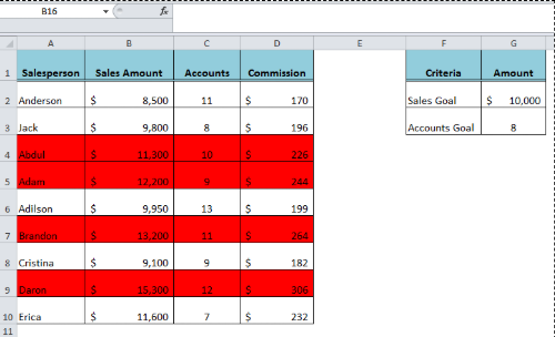
Figure 1. Final result
AND Function
The AND function is used to evaluate multiple conditions and it returns TRUE when all the conditions are met, otherwise returns FALSE. Therefore, the custom rule of conditional formatting with AND function triggers to highlight selected cells or rows when all the provided conditions are met. We have a dataset of salespersons accounts and their sales amounts. We want to evaluate the following conditions to highlight the rows where salespersons exceed both sales and account goals
- Sales Amounts in column B are greater than or equal (>=) to the Sales Goal of $10,000
- AND Accounts in column C are greater than or equal (>=) to the Accounts Goal of 8
Using conditional formatting with AND function the custom formula rule is created to evaluate both given conditions in the following formula syntax:
=AND(Sales Amount >=Sales Goal, Accounts >=Accounts Goal)
OR
=AND($B2>=$G$2,$C2>=$G$3)
 Figure 2. Salespersons’ dataset with conditions to evaluate
Applying Conditional Formatting
We use conditional formatting with AND function to highlight rows where above two conditions are met. To add conditional formatting in this case, follow the following steps:
- Select the range of cells where salespersons data is entered, such as A2: D10
- On the Home tab, click Conditional Formatting and then click New Rule
- Click the option “Use a Formula to Determine Which Cells to Format”
- In the formula box, enter
=AND($B2>=$G$2,$C2>=$G$3) - Click the Format button and select the Formatting option, such as Fill > Red color > OK
- Click OK
 Figure 3. Applying Conditional Formatting with AND function
Figure 4. Highlighting rows that meet both conditions
Instant Connection to an Expert through our Excelchat Service:
Most of the time, the problem you will need to solve will be more complex than a simple application of a formula or function. If you want to save hours of research and frustration, try our live Excelchat service! Our Excel Experts are available 24/7 to answer any Excel question you may have. We guarantee a connection within 30 seconds and a customized solution within 20 minutes.
Conditional formatting is a fantastic way to quickly visualize data in a spreadsheet. With conditional formatting, you can do things like highlight dates in the next 30 days, flag data entry problems, highlight rows that contain top customers, show duplicates, and more.
Excel ships with a large number of «presets» that make it easy to create new rules without formulas. However, you can also create rules with your own custom formulas. By using your own formula, you take over the condition that triggers a rule and can apply exactly the logic you need. Formulas give you maximum power and flexibility.
For example, using the «Equal to» preset, it’s easy to highlight cells equal to «apple».
But what if you want to highlight cells equal to «apple» or «kiwi» or «lime»? Sure, you can create a rule for each value, but that’s a lot of trouble. Instead, you can simply use one rule based on a formula with the OR function:

Here’s the result of the rule applied to the range B4:F8 in this spreadsheet:

Here’s the exact formula used:
=OR(B4="apple",B4="kiwi",B4="lime")
Quick start
You can create a formula-based conditional formatting rule in four easy steps:
1. Select the cells you want to format.

2. Create a conditional formatting rule, and select the Formula option

3. Enter a formula that returns TRUE or FALSE.

4. Set formatting options and save the rule.

The ISODD function only returns TRUE for odd numbers, triggering the rule:

Video: How to apply conditional formatting with a formula
Formula logic
Formulas that apply conditional formatting must return TRUE or FALSE, or numeric equivalents. Here are some examples:
=ISODD(A1)
=ISNUMBER(A1)
=A1>100
=AND(A1>100,B1<50)
=OR(F1="MN",F1="WI")
The above formulas all return TRUE or FALSE, so they work perfectly as a trigger for conditional formatting.
When conditional formatting is applied to a range of cells, enter cell references with respect to the first row and column in the selection (i.e. the upper-left cell). The trick to understanding how conditional formatting formulas work is to visualize the same formula being applied to each cell in the selection, with cell references updated as usual. Imagine that you entered the formula in the upper-left cell of the selection, and then copied the formula across the entire selection. If you struggle with this, see the section on Dummy Formulas below.
Formula Examples
Below are examples of custom formulas you can use to apply conditional formatting. Some of these examples can be created using Excel’s built-in presets for highlighting cells, but custom formulas can go far beyond presets, as you can see below.
Highlight orders from Texas
To highlight rows that represent orders from Texas (abbreviated TX), use a formula that locks the reference to column F:
=$F5="TX"

For more details, see this article: Highlight rows with conditional formatting.
Video: How to highlight rows with conditional formatting
Highlight dates in the next 30 days
To highlight dates occurring in the next 30 days, we need a formula that (1) makes sure dates are in the future and (2) makes sure dates are 30 days or less from today. One way to do this is to use the AND function together with the NOW function like this:
=AND(B4>NOW(),B4<=(NOW()+30))
With a current date of August 18, 2016, the conditional formatting highlights dates as follows:

The NOW function returns the current date and time. For details about how this formula, works, see this article: Highlight dates in the next N days.
Highlight column differences
Given two columns that contain similar information, you can use conditional formatting to spot subtle differences. The formula used to trigger the formatting below is:
=$B4<>$C4

See also: a version of this formula that uses the EXACT function to do a case-sensitive comparison.
Highlight missing values
To highlight values in one list that are missing from another, you can use a formula based on the COUNTIF function:
=COUNTIF(list,B5)=0

This formula simply checks each value in List A against values in the named range «list» (D5:D10). When the count is zero, the formula returns TRUE and triggers the rule, which highlights values in List A that are missing from List B.
Video: How to find missing values with COUNTIF
Highlight properties with 3+ bedrooms under $350k
To find properties in this list that have at least 3 bedrooms but are less than $300,000, you can use a formula based on the AND function:
=AND($C5<350000,$D5>=3)
The dollar signs ($) lock the reference to columns C and D, and the AND function is used to make sure both conditions are TRUE. In rows where the AND function returns TRUE, the conditional formatting is applied:

Highlight top values (dynamic example)
Although Excel has presets for «top values», this example shows how to do the same thing with a formula, and how formulas can be more flexible. By using a formula, we can make the worksheet interactive — when the value in F2 is updated, the rule instantly responds and highlights new values.

The formula used for this rule is:
=B4>=LARGE(data,input)
Where «data» is the named range B4:G11, and «input» is the named range F2. This page has details and a full explanation.
Gantt charts
Believe it or not, you can even use formulas to create simple Gantt charts with conditional formatting like this:

This worksheet uses two rules, one for the bars, and one for the weekend shading:
=AND(D$4>=$B5,D$4<=$C5) // bars
=WEEKDAY(D$4,2)>5 // weekends
This article explains the formula for bars, and this article explains the formula for weekend shading.
Simple search box
One cool trick you can do with conditional formatting is to build a simple search box. In this example, a rule highlights cells in column B that contain text typed in cell F2:

The formula used is:
=ISNUMBER(SEARCH($F$2,B2))
For more details and a full explanation, see:
- Article: How to highlight cells that contain specific text
- Article: How to highlight rows that contain specific text
- Video: How to build a search box to highlight data
Troubleshooting
If you can’t get your conditional formatting rules to fire correctly, there’s most likely a problem with your formula. First, make sure you started the formula with an equals sign (=). If you forget this step, Excel will silently convert your entire formula to text, rendering it useless. To fix, just remove the double quotes Excel added at either side and make sure the formula begins with equals (=).
If your formula is entered correctly but is not triggering the rule, you may have to dig a little deeper. Normally, you can use the F9 key to check results in a formula or use the Evaluate feature to step through a formula. Unfortunately, you can’t use these tools with conditional formatting formulas, but you can use a technique called «dummy formulas».
Dummy Formulas
Dummy formulas are a way to test your conditional formatting formulas directly on the worksheet, so you can see what they’re actually doing. This can be a big time-saver when you’re struggling to get cell references working correctly.
In a nutshell, you enter the same formula across a range of cells that matches the shape of your data. This lets you see the values returned by each formula, and it’s a great way to visualize and understand how formula-based conditional formatting works. For a detailed explanation, see this article.

Video: Test conditional formatting with dummy formulas
Limitations
There are some limitations that come with formula-based conditional formatting:
- You can’t apply icons, color scales, or data bars with a custom formula. You are limited to standard cell formatting, including number formats, font, fill color and border options.
- You can’t use certain formula constructs like unions, intersections, or array constants for conditional formatting criteria.
- You can’t reference other workbooks in a conditional formatting formula.
You can sometimes work around #2 and #3. You may be able to move the logic of the formula into a cell in the worksheet, then refer to that cell in the formula instead. If you are trying to use an array constant, try created a named range instead.
More CF formula resources
- More than 30 conditional formatting formulas examples
- Video training with practice worksheets
I am currently responsible for an Excel application with a lot of legacy code. One of the slowest pieces of this code was looping through 500 Rows in 6 Columns, setting conditional formatting formulae for each. The formulae are to identify where the cell contents are non-blank but do not form part of a Named Range, therefore referring twice to the cell itself, originally written as:
=AND(COUNTIF(<rangename>,<cellref>)=0,<cellref><>"")
Obviously the overheads would be much reduced by updating all Cells in each Column (Range) at once. However, as noted above, using ADDRESS(ROW(),COLUMN(),n) does not work in this circumstance, i.e. this does not work:
=AND(COUNTIF(<rangename>,ADDRESS(ROW(),COLUMN(),1))=0,ADDRESS(ROW(),COLUMN(),1)<>"")
I experimented extensively with a blank workbook and could find no way around this, using various alternatives such as ISBLANK. In the end, to get around this, I created two User-Defined Functions (using a tip I found elsewhere on this site):
Public Function returnCellContent() As Variant

  returnCellContent = Application.Caller.Value

End Function

Public Function Cell_HasContent() As Boolean

  If Application.Caller.Value = "" Then
    Cell_HasContent = False
  Else
    Cell_HasContent = True
  End If

End Function
The conditional formula is now:
=AND(COUNTIF(<rangename>,returnCellContent()=0,Cell_HasContent())
which works fine.
This has sped the code up, in Excel 2010, from 5s to 1s. Because this code is run whenever data is loaded into the application, this saving is significant and noticeable to the user. It’s also a lot cleaner and reusable.
I’ve taken the time to post this because I could not find any answers on this site or elsewhere that cover all of the circumstances, whilst I’m sure that there are others who could benefit from the above approach, potentially with much larger numbers of cells to update.
Conditional Formatting is one of the most simple yet powerful features in Excel Spreadsheets.
As the name suggests, you can use conditional formatting in Excel when you want to highlight cells that meet a specified condition.
It gives you the ability to quickly add a visual analysis layer over your data set. You can create heat maps, show increasing/decreasing icons, Harvey bubbles, and a lot more using conditional formatting in Excel.
Using Conditional Formatting in Excel (Examples)
In this tutorial, I’ll show you seven amazing examples of using conditional formatting in Excel:
- Quickly Identify Duplicates using Conditional Formatting in Excel.
- Highlight Cells with Value Greater/Less than a Number in a Dataset.
- Highlighting Top/Bottom 10 (or 10%) values in a Dataset.
- Highlighting Errors/Blanks using Conditional Formatting in Excel.
- Creating Heat Maps using Conditional Formatting in Excel.
- Highlight Every Nth Row/Column using Conditional Formatting.
- Search and Highlight using Conditional Formatting in Excel.
1. Quickly Identify Duplicates
Conditional formatting in Excel can be used to identify duplicates in a dataset.
Here is how you can do this:
This would instantly highlight all the cells that have a duplicate in the selected data set. Your dataset can be in a single column, multiple columns, or in a non-contiguous range of cells.

See Also: The Ultimate Guide to Find and Remove Duplicates in Excel.
2. Highlight Cells with Value Greater/Less than a Number
You can use conditional formatting in Excel to quickly highlight cells that contain values greater/less than a specified value. For example, highlighting all cells with sales value less than 100 million, or highlighting cells with marks less than the passing threshold.
Here are the steps to do this:
This would instantly highlight all the cells with values greater than 5 in a dataset. Note: If you wish to highlight values greater than equal to 5, you should apply conditional formatting again with the criteria “Equal To”.
The same process can be followed to highlight cells with a value less than a specified values.
3. Highlighting Top/Bottom 10 (or 10%)
Conditional formatting in Excel can quickly identify top 10 items or top 10% from a data set. This could be helpful in situations where you want to quickly see the top candidates by scores or top deal values in the sales data.
Similarly, you can also quickly identify the bottom 10 items or bottom 10% in a dataset.
Here are the steps to do this:
This would instantly highlight the top 10 items in the selected dataset. Note that this works only for cells that have a numeric value in it.
Also, if you have less than 10 cells in the dataset, and you select the options to highlight Top 10 items/Bottom 10 Items, then all the cells would get highlighted.
Here are some examples of how the conditional formatting would work:

4. Highlighting Errors/Blanks
If you work with a lot of numerical data and calculations in Excel, you’d know the importance of identifying and treating cells that have errors or are blank. If these cells are used in further calculations, it could lead to erroneous results.
Conditional Formatting in Excel can help you quickly identify and highlight cells that have errors or are blank.
Suppose we have a dataset as shown below:

This data set has a blank cell (A4) and errors (A5 and A6).
Here are steps to highlight the cells that are empty or have errors in it:
This would instantly highlight all the cells that are either blank or have errors in it.
 Note: You don’t need to use the entire range A1:A7 in the formula in conditional formatting. The above-mentioned formula only uses A1. When you apply this formula to the entire range, excel checks one cell at a time and adjusts the reference. For example, when it checks A1, it uses the formula =OR(ISBLANK(A1),ISERROR(A1)). When it checks cell A2, it then uses the formula =OR(ISBLANK(A2),ISERROR(A2)). It automatically adjusts the reference (as these are relative references) depending on which cell is being analyzed. So you need not write a separate formula for each cell. Excel is smart enough to change the cell reference all by itself 🙂
See Also: Using IFERROR and ISERROR to handle errors in excel.
5. Creating Heat Maps
A heat map is a visual representation of data where the color represents the value in a cell. For example, you can create a heat map where a cell with the highest value is colored green and there is a shift towards red color as the value decreases.
Something as shown below:

The above data set has values between 1 and 100. Cells are highlighted based on the value in it. 100 gets the green color, 1 gets the red color.
Here are the steps to create heat maps using conditional formatting in Excel.
- Select the data set.
- Go to Home –> Conditional Formatting –> Color Scales, and choose one of the color schemes.


As soon as you click on the heatmap icon, it would apply the formatting to the dataset. There are multiple color gradients that you can choose from. If you are not satisfied with the existing color options, you can select more rules and specify the color that you want.
Note: In a similar way, you can also apply Data Bard and Icon sets.
6. Highlight Every Other Row/Column
You may want to highlight alternate rows to increase the readability of the data.
These are called the zebra lines and could be especially helpful if you are printing the data.
Now there are two ways to create these zebra lines. The fastest way is to convert your tabular data into an Excel Table. It automatically applied a color to alternate rows. You can read more about it here.
Another way is using conditional formatting.
Suppose you have a dataset as shown below:

Here are the steps to highlight alternate rows using conditional formatting in Excel.
That’s it! The alternate rows in the data set will get highlighted.

You can use the same technique in many cases. All you need to do is use the relevant formula in the conditional formatting. Here are some examples:
- Highlight alternate even rows: =ISEVEN(ROW())
- Highlight alternate add rows: =ISODD(ROW())
- Highlight every 3rd row: =MOD(ROW(),3)=0
7. Search and Highlight Data using Conditional Formatting
This one is a bit advanced use of conditional formatting. It would make you look like an Excel rockstar.
Suppose you have a dataset as shown below, with Products Name, Sales Rep, and Geography. The idea is to type a string in cell C2, and if it matches with the data in any cell(s), then that should get highlighted. Something as shown below:

Here are the steps to create this Search and Highlight functionality:
That’s it! Now when you enter anything in cell C2 and hit enter, it will highlight all the matching cells.
How does this work?
The formula used in conditional formatting evaluates all the cells in the dataset. Let’s say you enter Japan in cell C2. Now Excel would evaluate the formula for each cell.
The formula would return TRUE for a cell when two conditions are met:
- Cell C2 is not empty.
- The content of cell C2 exactly matches the content of the cell in the dataset.
Hence, all the cells that contain the text Japan get highlighted.
Download the Example File

You can use the same logic, to create variations such as:
- Highlight the entire row instead of a cell.
- Highlight even when there is a partial match.
- Highlight the cells/rows as you type (dynamic) [You are going to love this trick :)].
How to Remove Conditional Formatting in Excel
Once applied, conditional formatting remains in place unless you remove it manually. As a best practice, keep the conditional formatting applied only to those cells where you need it.
Since it’s volatile, it may lead to a slow Excel workbook.
To remove conditional formatting:
- Select the cells from which you want to remove conditional formatting.
- Go to Home –> Conditional Formatting –> Clear Rules –> Clear Rules from Selected Cells.
- If you want to remove conditional formatting from the entire worksheet, select Clear Rules from Entire Sheet.

- If you want to remove conditional formatting from the entire worksheet, select Clear Rules from Entire Sheet.

Important things to know about Conditional Formatting in Excel
- Conditional formatting in volatile. It can lead to a slow workbook. Use it only when needed.
- When you copy paste cells that contain conditional formatting, conditional formatting also gets copied.
- If you apply multiple rules on the same set of cells, all rules remain active. In the case of any overlap, the rule applied last is given preference. You can, however, change the order by changing the order from the Manage Rules dialogue box.
You May Also Like the Following Excel Tutorials:
- The Right Way to Apply Conditional Formatting in Pivot Table
- Find and Remove Duplicates in Excel
- The Ultimate Guide to Using Conditional Formatting in Google Sheets
- How to Highlight Weekend Dates in Excel?